Modal decomposition of astronomical images with application to shapelets

Abstract

The decomposition of an image into a linear combination of digitised basis functions is an everyday task in astronomy. A general method is presented for performing such a decomposition optimally into an arbitrary set of digitised basis functions, which may be linearly dependent, non-orthogonal and incomplete. It is shown that such circumstances may result even from the digitisation of continuous basis functions that are orthogonal and complete. In particular, digitised shapelet basis functions are investigated and are shown to suffer from such difficulties. As a result the standard method of performing shapelet analysis produces unnecessarily inaccurate decompositions. The optimal method presented here is shown to yield more accurate decompositions in all cases.

1 Introduction

The linear decomposition of an astronomical dataset into a series of basis functions is a fundamental task in many areas of astrophysics and cosmology. Indeed, in the analysis of one-dimensional spectra, two-dimensional images or higher-dimensional datasets, one is often faced with the problem of determining the coefficients in a linear expansion of the dataset in some set of (sampled) basis functions. To illustrate our discussion, we will focus here on the important specific example of decomposing a two-dimensional astronomical image, although the general approach that we advocate will be applicable to datasets of arbitrary dimensionality.

The description of a digitised image as a linear combination of a set of sampled basis functions is an everyday problem for astronomers. For example, one often describes an image in terms of a set of orthogonal Fourier modes by calculating the coefficients in the expansion using a discrete Fourier transform. Significant attention has also been given to representing an image as a linear combination of discrete wavelets basis functions, both orthogonal and non-orthogonal (see, for instance, Hobson et al. 1999; Sanz et al 1999a;b; Tenorio et al. 1999). More recently, several authors have investigated the use of Gaussian-Hermite modes (or shapelets) in representing images of galaxies (Refregier 2003; Refregier & Bacon 2003). Although such image decompostion is commonplace, there exist a number of subtleties in the procedure that are not widely appreciated within the astronomical community. These include the effect of digitisation, or sampling, on familiar notions from the analytic theory of continuous functions, in particular the concepts of completeness and linear independence of sampled basis functions, and the use of non-orthogonal bases.

In this paper, we therefore discuss a general mathematical framework for the linear decomposition of an astronomical image into a set of arbitrary sampled functions (or modes). These may, in general, form a ‘basis’ that is non-orthogonal and either under-complete, perfectly-complete or over-complete. In the under-complete case, the modes do not support all the degrees of freedom in an arbitrary image. By perfectly-complete we mean that the modes supports all the degrees of freedom without linear dependence between them, whereas for an over-complete mode set there are additional modes relative to the complete case and hence linear dependence in the set. In particular, we show how to quantify those degrees of freedom in an image that can be supported by any particular mode set, and we explicitly consider how to obtain the optimal set of mode coefficients for representing the image. These methods present an opportunity for the optimisation of sampling within modal analysis, ensuring that computational operations are reduced to a minimum.

The structure of the paper is as follows. In Section 2, we outline the modal decomposition problem and present a general prescription for obtaining optimal results, which is based on the singular value decomposition of the matrix of digitised mode vectors. In Section 3, we illustrate our general approach by investigating the decomposition of simple one-dimensional function into Gauss-Hermite (shapelet) modes. This investigation is pursued further in Section 4, where we consider the decomposition of images of Hubble Deep Field galaxies into two-dimensional Gauss-Laguerre (polar shapelet) modes. Finally, our conclusions are presented in section 5.

2 The modal decomposition problem

Consider a 2-D digitised image consisting of $N$ pixels, which we denote by the $N$-dimensional column vector d. Our goal is to represent the image, as accurately as possible, in terms of a set of $M$ (two-dimensional) modes $\{{\textbf{{e}}}_{k}\}$ $(k=1,2,\ldots,M)$ defined at the same points at which d is sampled; thus each ${\textbf{{e}}}_{k}$ is also a column vector of length $N$. It is convenient to combine the mode vectors into the single $N\times M$ mode matrix defined by

$${\textbf{{E}}}=[{\textbf{{e}}}_{1}\cdots{\textbf{{e}}}_{k}\cdots{\textbf{{e}}}_{M}].$$

Our objective is thus to determine a suitable coefficient vector $\hat{{\textbf{{a}}}}$ that minimises the residual

$$\epsilon=|{\textbf{{E}}}{\textbf{{a}}}-{\textbf{{d}}}|.$$ (1)

Note that we make no requirement for the mode vectors to be mutually orthogonal, linearly independent, or of unit length.

Several cases may arise in this problem. There may exist a unique coefficient vector $\hat{{\textbf{{a}}}}$ that minimises (1); this corresponds to the quantity $\epsilon^{2}$ possessing a single well-defined multi-dimensional quadratic minimum in the space of coefficients a. Surfaces of constant $\epsilon^{2}$ are given by the Hermitian form $({\textbf{{a}}}-\hat{{\textbf{{a}}}})^{\dagger}{\textbf{{R}}}({\textbf{{a}}}-\hat{{\textbf{{a}}}})=\mbox{constant}$, where ${\textbf{{R}}}={\textbf{{E}}}^{\dagger}{\textbf{{E}}}$ (which is called the Gram matrix). The eigenvectors of R determine the principal directions of this multi-dimensional ellipsoid, and the extent along each principal direction is inversely proportional to the corresponding eigenvalue. If there exist approximate degeneracies in the coefficient-space, some of the eigenvalues become very small and so the multi-dimensional ellipsoid is considerably elongated in these directions; this leads to a wide range of coefficients vectors a for which $\epsilon$ takes its minimum value to within the numerical precision. In the limiting case of exact degeneracies, some eigenvalues are identically zero leading to an infinite extent for the ‘ellipsoid’ along the corresponding principal directions. In the subspace spanned by these directions the value of $\epsilon$ takes its minimum value precisely. In either of the last two cases, to the numerical precision, there exist an infinite number of possible coefficient vectors $\hat{{\textbf{{a}}}}$ that minimise (1). The value of $\epsilon_{\rm min}$ is also of central importance. Clearly, if $\epsilon_{\rm min}=0$, then the modal expansion ${\textbf{{E}}}\hat{{\textbf{{a}}}}$ provides an exact representation of the original image, whereas if $\epsilon_{\rm min}>0$ it represents only an approximation to d.

Which of the above cases occurs is dependent on the completeness and linear dependence of the mode set ${{\textbf{{e}}}_{k}}$, and on the particular image d being decomposed. Clearly, if the $M<N$ then the modes are ‘under-complete’, and so cannot represent an arbitrary image, but only an approximation to it. This may also occur when $M\geq N$, however, since the modes may still not form a complete basis as a result of linear dependence between them. Nevertheless, even with an under-complete set, the particular image d under analysis may lie in the subspace spanned by the modes, and so may be represented exactly. When $M\geq N$ cases arise where the modes form a complete basis, in which any image can be represented exactly. In this case, if $M=N$ the modes must linearly independent and form a ‘perfectly-complete’ basis. If $M>N$, some linear dependence must exist between the modes and they form an ‘over-complete’ basis.

In general, the degree of completeness of the chosen mode set may not be known at the outset. Fortunately, a straightforward technique exists for determining the degree of completeness of the mode set, and simultaneously determining an ‘appropriate’ coefficient vector $\hat{{\textbf{{a}}}}$ that minimises (1). This is achieved by performing the singular-value decomposition (SVD) of the mode matrix E, which we now discuss.

2.1 Singular value decomposition

The SVD of the $N\times M$ mode matrix E (which may, in general, contain complex-valued entries) may be written (see, for example, Golub & Van Loan 1992)

$${\textbf{{E}}}={\textbf{{U}}}{\mbox{\bf$\Sigma$}}{\textbf{{V}}}^{\dagger},$$ (2)

where U is unitary matrix of dimensions $N\times N$, V is a unitary matrix of dimensions $M\times M$, and $\Sigma$ is a $N\times M$ matrix (the same dimensions as E) that is diagonal in the sense that $\Sigma_{ii}=\sigma_{i}$ for $i\leq p$, where $p=\mbox{min}[M,N]$, and zero otherwise. The coefficients $\sigma_{i}$ are the singular values of the matrix E.

As is well-known, the number $r$ (say) of non-zero singular values is equal to the rank of E, which in turn is the dimensionality of the image subspace that is spanned by the $M$ modes $\{{\textbf{{e}}}_{k}\}$; clearly it must be the case that $r\leq M$ and $r\leq N$. The dimensionality of the nullspace of E (the subspace of vectors n in the coefficient space for which ${\textbf{{E}}}{\textbf{{n}}}={\textbf{{0}}}$) is given by $M-r$. It is thus a simple matter to determine the completeness of the mode set contained in E as follows: (i) if $r<N$ the modes are under-complete; (ii) if $r=N$ and $M=N$ the modes are perfectly complete; and (iii) if $r=N$ and $M>N$ the modes are over-complete. Moreover, it is straightforward to show that the columns of U corresponding to non-zero singular values constitute an orthonormal basis for the range of E, and the columns of V that do not correspond to a non-zero singular value form an orthonormal basis for the nullspace. In practical numerical problems, it is often the case that none of the singular values $\sigma_{i}$ are identically zero. Instead, one usually sets to zero those singular values for which $|\sigma_{i}|/|\sigma_{1}|<\eta$, where $\eta$ is some small factor (for example, $10^{-5}$ in single precision arithmetic) and $\sigma_{1}$ is the first (and largest) singular value.

Once the SVD (2) has been calculated, it is also straightforward to obtain an ‘appropriate’ coefficient vector $\hat{{\textbf{{a}}}}$ that minimises (1). As we outline below, in all cases one should calculate the coefficient vector using

$$\hat{{\textbf{{a}}}}={\textbf{{V}}}\overline{{\mbox{\bf$\Sigma$}}}^{\dagger}{\textbf{{U}}}^{\dagger}{\textbf{{d}}},$$ (3)

where the $M\times N$ matrix denoted by $\overline{{\mbox{\bf$\Sigma$}}}^{\dagger}$ is constructed by taking the transpose of $\Sigma$ in (2) and replacing each non-zero singular value $\sigma_{i}$ by $1/\sigma_{i}$.

It is clear that, with the above construction, ${\mbox{\bf$\Sigma$}}\overline{{\mbox{\bf$\Sigma$}}}^{\dagger}$ is an $N\times N$ diagonal matrix with diagonal entries that equal unity for those values of $j$ for which $\sigma_{j}\neq 0$, and zero otherwise. Using this result it is straightforward to show that (3) does indeed minimise the residual (1). Modifying slightly the argument of Press et al. (1994), suppose we were to add to $\hat{{\textbf{{a}}}}$ some arbitrary vector ${\textbf{{a}}}^{\prime}={\textbf{{a}}}_{1}^{\prime}+{\textbf{{a}}}_{2}^{\prime}$, where ${\textbf{{a}}}_{2}^{\prime}$ is the part of the vector that lies in the nullspace of E (if one exists) and ${\textbf{{a}}}_{1}^{\prime}$ is the part that lies in the complement to the nullspace. This would result in the addition of the vector ${\textbf{{d}}}^{\prime}={\textbf{{E}}}{\textbf{{a}}}_{1}^{\prime}$ to ${\textbf{{E}}}\hat{{\textbf{{a}}}}-{\textbf{{d}}}$. We would then have

$$|{\textbf{{E}}}\hat{{\textbf{{a}}}}-{\textbf{{d}}}+{\textbf{{d}}}^{\prime}| = |({\textbf{{U}}}{\mbox{\bf$\Sigma$}}\overline{{\mbox{\bf$\Sigma$}}}^{\dagger}{\textbf{{U}}}^{\dagger}-{\textbf{{I}}}){\textbf{{d}}}+{\textbf{{d}}}^{\prime}|$$ (4)

$$= |{\textbf{{U}}}[({\mbox{\bf$\Sigma$}}\overline{{\mbox{\bf$\Sigma$}}}^{\dagger}-{\textbf{{I}}}){\textbf{{U}}}^{\dagger}{\textbf{{d}}}+{\textbf{{U}}}^{\dagger}]{\textbf{{d}}}^{\prime}|$$

$$= |({\mbox{\bf$\Sigma$}}\overline{{\mbox{\bf$\Sigma$}}}-{\textbf{{I}}}){\textbf{{U}}}^{\dagger}{\textbf{{d}}}+{\textbf{{U}}}^{\dagger}{\textbf{{d}}}^{\prime}|,$$

where in the last line we have made use of the fact that the length of a vector is left unchanged under the action of the unitary matrix U. Now, the $j$th component of the vector $({\mbox{\bf$\Sigma$}}\overline{{\mbox{\bf$\Sigma$}}}-{\textbf{{I}}}){\textbf{{U}}}^{\dagger}{\textbf{{d}}}$ will only be non-zero when $\sigma_{j}=0$. However, the $j$th element of the vector ${\textbf{{U}}}^{\dagger}{\textbf{{d}}}^{\prime}$ is non-zero only if $\sigma_{j}\neq 0$, since ${\textbf{{d}}}^{\prime}$ lies in the range of E. Thus, as these two terms only contribute to (4) for two disjoint sets of $j$-values, its minimum value, as ${\textbf{{a}}}^{\prime}$ is varied, occurs when ${\textbf{{d}}}^{\prime}={\textbf{{0}}}$; this requires ${\textbf{{a}}}_{1}^{\prime}={\textbf{{0}}}$.

If the image d lies in the subspace spanned by the $M$ modes $\{{\textbf{{e}}}_{k}\}$, then the minimum value of the residual (1) is zero, and the image is represented exactly by ${\textbf{{E}}}\hat{{\textbf{{a}}}}$. Clearly, in order to represent an arbitrary image we require $r=N$ (and so $M\geq N$). If d does not lie in the range of E, then ${\textbf{{E}}}\hat{{\textbf{{a}}}}$ yields only an approximate representation of the image (for this to occur, the modes must be under-complete; this will always be true if $M<N$, but may also occur when $M\geq N$).

In either case, we see from the argument above that, if E does not possess a null space, the coefficient vector (3) is unique in minimising the residual (1). The condition for this to occur is that $r=M$, indicating that the $M$ modes are linearly independent (and hence requiring $M\leq N$). If E does possess a nullspace, however, any vector ${\textbf{{a}}}_{2}^{\prime}$ in this nullspace can be added to (3), without changing the value of the residual. Thus there are an infinite number of coefficient vectors that minimise (1). The condition for this to occur is that $r<M$, indicating linear dependence between the modes (which may occur for $M\leq N$ and $M>N$).

In the case where ${\bf E}$ possesses a nullspace, from the infinite number of coefficient vectors that minimise the residual (1), the vector $\hat{{\textbf{{a}}}}$ in (3) is that which contains no contribution from the nullspace. An equivalent statement is that (3) is the vector of shortest length that minimises (1). Consider again adding some arbitrary vector ${\textbf{{a}}}^{\prime}$ to (3). The length of the resulting vector is

$$|\hat{{\textbf{{a}}}}+{\textbf{{a}}}^{\prime}| = |{\textbf{{V}}}\overline{{\mbox{\bf$\Sigma$}}}^{\dagger}{\textbf{{U}}}^{\dagger}{\textbf{{d}}}+{\textbf{{a}}}^{\prime}|$$

$$= |{\textbf{{V}}}(\overline{{\mbox{\bf$\Sigma$}}}^{\dagger}{\textbf{{U}}}^{\dagger}{\textbf{{d}}}+{\textbf{{V}}}^{\dagger}{\textbf{{a}}}^{\prime})|$$

$$= |\overline{{\mbox{\bf$\Sigma$}}}^{\dagger}{\textbf{{U}}}^{\dagger}{\textbf{{d}}}+{\textbf{{V}}}^{\dagger}{\textbf{{a}}}^{\prime}|,$$

where in the last line we again make use of the fact that the length of a vector is left unchanged under the action of a unitary matrix. The $j$th component of the vector $\overline{{\mbox{\bf$\Sigma$}}}{\textbf{{U}}}^{\dagger}{\textbf{{d}}}$ will only be non-zero when $\sigma_{j}\neq 0$, whereas the $j$th element of the vector ${\textbf{{V}}}^{\dagger}{\textbf{{a}}}^{\prime}$ is non-zero only if $\sigma_{j}=0$. Thus the minimum length vector has ${\textbf{{a}}}^{\prime}={\textbf{{0}}}$.

2.2 Dual modes

Although the appropriate coefficient vector may always be obtained straightforwardly from (3), it is conceptually appealing to consider coefficient $\hat{a}_{k}$ as the scalar product of the image vector d with some new mode vector $\tilde{{\textbf{{e}}}}_{k}$ that is dual to the original mode ${\textbf{{e}}}_{k}$. In other words, it is often convenient to rewrite (3) as

$$\hat{{\textbf{{a}}}}=\tilde{{\textbf{{E}}}}^{\dagger}{\textbf{{d}}},$$ (5)

where $\tilde{{\textbf{{E}}}}$ is the $N\times M$ dual mode matrix, which contains the $M$ dual mode vectors as its columns, i.e.

$$\tilde{{\textbf{{E}}}}=[\tilde{{\textbf{{e}}}}_{1}\cdots\tilde{{\textbf{{e}}}}_{k}\cdots\tilde{{\textbf{{e}}}}_{M}].$$

From (3), we see immediately that the dual mode matrix is given in terms of the SVD of the original mode matrix by

$$\tilde{{\textbf{{E}}}}={\textbf{{U}}}\overline{{\mbox{\bf$\Sigma$}}}{\textbf{{V}}}^{\dagger}.$$

Thus, once a mode set has been defined, the dual mode set can be calculated directly by performing a SVD, without reference to any image. The coefficients for any particular image are then quickly obtained using (5).

It should be noted that, in general,

$${\textbf{{E}}}\tilde{{\textbf{{E}}}}^{\dagger}\neq{\textbf{{I}}}_{N}\neq\tilde{{\textbf{{E}}}}{\textbf{{E}}}^{\dagger},$$

where we now start to place subscripts on identity matrices to emphasise their dimensionality. It is only in the case where the original mode set is complete that ${\mbox{\bf$\Sigma$}}\overline{{\mbox{\bf$\Sigma$}}}^{\dagger}={\textbf{{I}}}_{N}=\overline{{\mbox{\bf$\Sigma$}}}{\mbox{\bf$\Sigma$}}^{\dagger}$, from which it is a simple matter to verify that ${\textbf{{E}}}\tilde{{\textbf{{E}}}}^{\dagger}={\textbf{{I}}}_{N}=\tilde{{\textbf{{E}}}}{\textbf{{E}}}^{\dagger}.$ This, of course, corresponds to the case in which an arbitrary image d can be represented exactly, since then

$${\textbf{{E}}}\hat{{\textbf{{a}}}}={\textbf{{E}}}\tilde{{\textbf{{E}}}}^{\dagger}{\textbf{{d}}}={\textbf{{d}}}.$$

Otherwise only an approximation to the original image is possible.

It is also worth pointing out that, in general,

$${\textbf{{E}}}^{\dagger}\tilde{{\textbf{{E}}}}\neq{\textbf{{I}}}_{M}\neq\tilde{{\textbf{{E}}}}^{\dagger}{\textbf{{E}}}.$$

In other words, the dual modes do not necessarily obey the standard orthogonality condition ${\textbf{{e}}}_{k}^{\dagger}\tilde{{\textbf{{e}}}}_{l}=\delta_{kl}=\tilde{{\textbf{{e}}}}_{k}^{\dagger}{\textbf{{e}}}_{l}$ with the original mode set. This orthogonality condition is only satisfied if the original mode set is linearly-independent (for which $r=M$ and hence $M\leq N$). In this case, ${\mbox{\bf$\Sigma$}}^{\dagger}\overline{{\mbox{\bf$\Sigma$}}}={\textbf{{I}}}_{M}=\overline{{\mbox{\bf$\Sigma$}}}^{\dagger}{\mbox{\bf$\Sigma$}}$, from which one quickly finds that ${\textbf{{E}}}^{\dagger}\tilde{{\textbf{{E}}}}={\textbf{{I}}}_{M}=\tilde{{\textbf{{E}}}}^{\dagger}{\textbf{{E}}}$, which recovers the standard result that the dual modes form the reciprocal basis of the original mode set. This corresponds to the case where (5) is unique in minimising the residual (1). If, in addition, we have $M=N$ and so the basis perfectly complete, E is invertible and it follows that $\tilde{{\textbf{{E}}}}^{\dagger}={\textbf{{E}}}^{-1}$. We reiterate, however, that all possible cases are automatically accommodated using SVD.

2.3 Orthogonal mode sets

So far, we have imposed no restrictions on the orthogonality, normalisation or the number of members of our original mode set $\{{\textbf{{e}}}_{k}\}$. It is worth investigating, however, the simplifications that occur in the case where the modes are mutually orthogonal and each mode is unique (so $M\leq N$). Hence, we have ${\textbf{{E}}}^{\dagger}{\textbf{{E}}}={\textbf{{I}}}_{M}$.

In this case, the mode set is automatically linearly-independent and so the coefficient vector (3) or (5) is unique in minimising the residual. Moreover, the dual modes and original modes obey the standard orthogonality condition ${\textbf{{E}}}^{\dagger}\tilde{{\textbf{{E}}}}={\textbf{{I}}}_{M}=\tilde{{\textbf{{E}}}}^{\dagger}{\textbf{{E}}}$. In the case of orthogonal modes, it is clear that, in addition, this condition is satisfied if the dual modes are given by

$$\tilde{{\textbf{{e}}}}_{k}=\frac{{\textbf{{e}}}_{k}}{|{\textbf{{e}}}_{k}|^{2}}.$$

Thus, for orthogonal modes (even with $M<N$), we see that each dual is simply proportional to the original mode. In the event that the original modes are normalised to unit length, this proportionality becomes an equality, and the dual modes are identical to the original modes, so that $\tilde{{\textbf{{E}}}}={\textbf{{E}}}$ and hence

$$\hat{{\textbf{{a}}}}={\textbf{{E}}}^{\dagger}{\textbf{{d}}}.$$ (6)

This last result is, of course, the reason for the common practice, in the case of orthonormal modes, of calculating the $k$th mode coefficient $\hat{a}_{k}$ by simply evaluating the scalar product of the image d with the $k$th mode ${\textbf{{e}}}_{k}$. Of course, when $M=N$, a set of orthogonal modes also forms a perfectly complete basis.

2.4 Practical considerations

Throughout our discussion, we have adopted the practical approach of working with finite dimensional vectors, rather than continous functions. Thus, both the image d and the modes ${\textbf{{e}}}_{k}$ are considered simply as $N$-dimensional vectors. This allows the direct application of our approach to a wide variety problems in the decomposition of digital astronomical images. The image pixel values $d_{i}$ correspond to samples of the underlying continuous distribution $d({\textbf{{x}}})$ at a particular set of points $\{{\textbf{{x}}}_{i}\}$. In practice, it is most often the case that sample points are regularly spaced, but this restriction is not necessary. The entire approach can just as easily be applied to the case where the pixels values correspond to samples that are not regularly spaced. In an analogous manner, the elements of each mode vector ${\textbf{{e}}}_{k}$ are the sample values from some underlying continuous mode function $f_{k}({\textbf{{x}}})$ at the same set of points $\{{\textbf{{x}}}_{i}\}$.

It is clear that the positions of the sample points will have a profound effect on whether the linear-independence, orthogonality, or other properties of the original set of continuous mode functions $\{f_{k}({\textbf{{x}}})\}$ are inherited by the mode vectors $\{{\textbf{{e}}}_{k}\}$. Consider, for example, a set of continuous mode functions $\{f_{k}({\textbf{{x}}})\}$ that are orthonormal over some continuous domain ${\cal D}$, so that

$$\int_{\cal D}f^{\ast}_{k}({\textbf{{x}}})f_{l}({\textbf{{x}}})\,{\rm d}{\textbf{{x}}}=\delta_{kl}.$$

Even in the case where the sample points $\{{\textbf{{x}}}_{i}\}$ are evenly spaced, the spacing between them and the extent of the domain ${\cal D}$ that is sampled are important in determining whether the corresponding mode vectors $\{{\textbf{{e}}}_{k}\}$ are orthonormal. Indeed, as we shall see below, in some applications it is common for the corresponding mode vectors not to be orthonormal. If this is the case, then it is is no longer true that the dual mode vectors are identical to the original mode vectors, and so it is incorrect to calculate the coefficient vector $\hat{{\textbf{{a}}}}$ using (6), i.e. by taking the scalar product of the data d with the mode vectors. This will lead to a modal decomposition of the image that is unnecessarily inaccurate. Instead, one must return to using the general result (5), where the mode coefficients are calculated by taking the scalar product of the data with the corresponding dual mode vectors.

Finally, a crucial point is that the converse may also occur. For example, if a set of continous mode functions are not orthogonal, by sampling them at a particular set of (non-uniform) points one can arrive at a set of mode vectors that are orthogonal, in which case the duals are trivially obtained.

3 One-dimensional illustrations

Although the main focus of this paper is the modal decompostion of two-dimensional astronomical images, it will be informative first to illustrate the discussion given above by investigating the decompostion of one-dimensional sampled functions (which may be considered as cuts through some image). In particular, we will focus our numerical investigations in this section on decompostions using one-dimensional Gaussian-Hermite (or shapelet) mode functions, as recently advocated by Refregier (2003) for representing images of galaxies.

In this case, the continuous mode functions are given by

$$f_{k}(x;\beta)=\beta^{-1/2}\phi_{k}(\beta^{-1}x),$$

for $k=0,1,2,\ldots,\infty$. The quantity $\beta$ is some fixed ‘characteristic scale’ for the set of mode functions and the function $\phi_{k}(u)$ reads

$$\phi_{k}(u)=(2^{k}\pi^{1/2}k!)^{-1/2}H_{k}(u)\exp(-u^{2}/2),$$

where $H_{k}(u)$ is a Hermite polynomial of order $k$. From these expressions it is clear that the mode functions are real and that $\beta$ is equal to the dispersion ‘$\sigma$’ of the $k=0$ Gaussian mode function. It is also straightforward to show that the mode functions are orthonormal over the domain $-\infty<x<\infty$, i.e.

$$\int_{-\infty}^{\infty}f_{k}(x;\beta)f_{l}(x;\beta)\,{\rm d}x=\delta_{kl}.$$ (7)

We note that, for convenience, the mode functions are centred at $x=0$. It is, of course, possible to centre them about some arbitrary point $x=x_{c}$, but in most cases the coordinate system is chosen so that the centroid of the galaxy image (say) is located at the origin. The first six mode functions are shown in Fig. 1 for $\beta=12$.

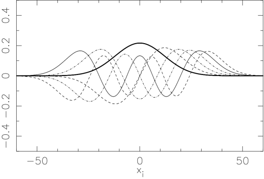
Figure 1: The Gaussian-Hermite continuous mode functions $f_{k}(x;\beta)$ for $k=0,1,\ldots,5$ and $\beta=12$.

Let us now consider the decomposition of a one-dimensional pixelised ‘image’ into shapelets. In any such decomposition, one is free to choose both the characteristic scale $\beta$ of the modes set and the total number $M$ of modes used (note that $M=k_{\rm max}+1$). As shown by Refregier (2003), such a set of shapelet modes is suitable for describing features in an image on scales between the two limits

$$\theta_{\rm min}\approx\beta M^{-1/2},\qquad\theta_{\rm max}\approx\beta M^{1/2}.$$ (8)

Thus, if the image has features on scales ranging from $\theta_{\rm min}$ (e.g. the pixel size or the size of the point spread function) to $\theta_{\rm max}$ (e.g. the size of the image or the overall extent of the structure it contains), then a good choice of $\beta$ and $M$ is

$$\beta\approx(\theta_{\rm min}\theta_{\rm max})^{1/2},\qquad M\approx\frac{\theta_{\rm max}}{\theta_{\rm min}}.$$ (9)

For each of the pixelised test images we consider below, we take the coordinate positions of the $N$ (regularly-spaced) sample points to be

$$\{x_{i}\}=\{-{\textstyle\frac{1}{2}}(N-1),\ldots,-1,0,1,\ldots,{\textstyle\frac{1}{2}}(N-1)\},$$

thereby giving an image of spatial extent of $N$, with a pixel size of unity. In each case, we take $N=81$. Taking into account that our test images contain structure on the order of the image size, but do not contain structure on scales less than a few pixels, acceptable choices for the scale parameter and the number of modes to use are $\beta\approx 10$ and $M\approx 20$. For convenience, we fix $M=20$, and investigate mode sets for which $\beta=1$ – 20 in steps of unity. In each case, the elements of the corresponding pixelised mode vectors are easily calculated from $({\textbf{{e}}}_{k})_{i}=f_{k}(x_{i};\beta)$.

In Fig. 2 we plot the elements of the first six mode vectors for $\beta=12$.

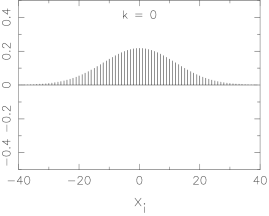
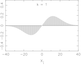
Figure 2: The Gaussian-Hermite mode vectors ${\textbf{{e}}}_{k}$ for $k=0,1,\ldots,5$ and $\beta=12$.

We see that, even for this modest value of $\beta$, the support of the mode vectors for $k>2$ exceeds the length of the image. Indeed, as $k$ increases the support of the mode vectors increases according to (8), and so this effect becomes extremely pronounced for the high-$k$ modes. As a result, we would expect the mode set does not satisfy the discretized form of the orthogonality condition (7). We will show below that this is indeed the case.

It is also of interest to investigate the structure of the mode vectors for different values of $\beta$. As an illustration, in Fig. 3 we plot the highest-$k$ mode vector in the set ($k_{\rm max}=19$) for six different values of the scale parameter $\beta$.

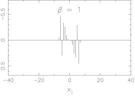
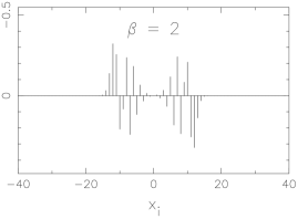
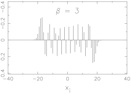
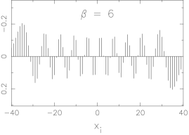
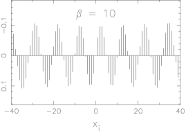
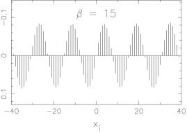
Figure 3: The $k_{\rm max}=19$ Gaussian-Hermite mode vector ${\textbf{{e}}}_{19}$ for $\beta=0,1,2,3,6,10,15$.

In particular, we note that the mode vector is severely undersampled for $\beta=1$ and $\beta=2$, in which case the mode set may again fail to be orthogonal. Moreover, since the highest-$k$ mode in the set has the largest spatial extent, we see that, in fact, for $\beta\geq 6$ the support of the mode set exceeds the length of the image, once again suggesting a loss of orthogonality.

3.1 Properties of the mode vectors

Since we have chosen $M<N$, the mode vectors clearly cannot form a complete basis for the image space. Nevertheless, it is of interest to investigate formally the linear-dependence and orthogonality of the mode vectors ${\textbf{{e}}}_{k}$ $(k=0,1,\ldots,M-1)$ for various values of the scale parameter $\beta$. To this end, for each value of $\beta$ under consideration, we construct the corresponding mode matrix E and then determine its rank $r$ by calculating its SVD and counting the number of non-zero singular values. If the mode vectors are linearly independent, one would expect $r=M$. In Fig. 4, we plot the value of $r$ as a function of the parameter $\beta$.

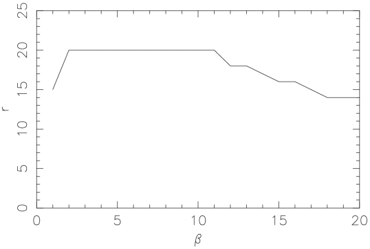
Figure 4: The rank $r$ of the mode matrix E as a function of the scale parameter $\beta$ for $M=20$ Gaussian-Hermite mode vectors.

Since the number of mode vectors is $M=20$, we see that the mode vectors form a linearly-independent $(r=20)$ set only if the scale parameter lies in the range $\beta=2$–11. For smaller values of $\beta$, the undersampling of the underlying continuous mode functions leads to linear dependence in the resulting mode set. For large $\beta$, linear dependence occurs since the support of (some of) the mode vectors exceeds the length of the image.

To investigate whether the mode vectors are orthonormal we calculate the Gram matrix ${\textbf{{R}}}={\textbf{{E}}}^{\dagger}{\textbf{{E}}}$ for each value of $\beta$ under consideration. Clearly, for an orthonormal set of mode vectors would expect ${\textbf{{R}}}={\textbf{{I}}}_{M}$. In Fig 5 (top), for each value of $\beta$, we plot the logarithms of the largest and smallest diagonal elements of R. For mode vectors of unit length, we would expect all the diagonal elements to equal unity, and so the two plotted curves should coincide at $\log(R_{ii})=0$. We see that this occurs only if the scale parameter lies in the range $\beta=3$–6.

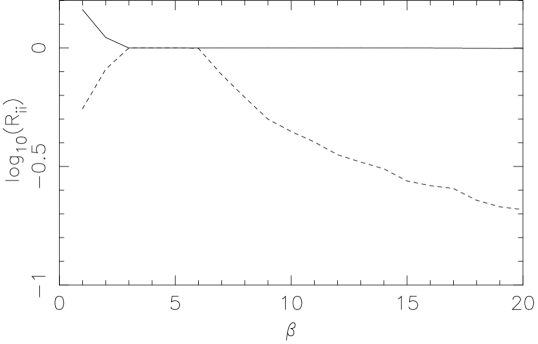
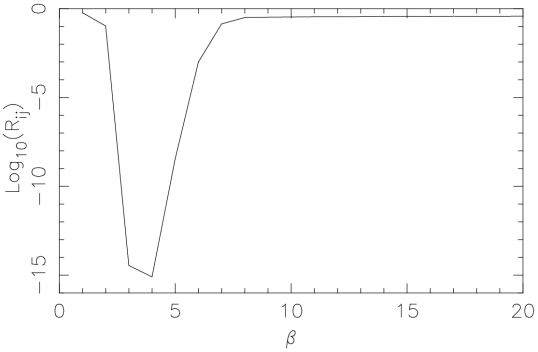
Figure 5: Top: the logarithm of the value of the largest (solid line) and smallest (dashed line) diagonal elements of the Gram matrix ${\textbf{{R}}}={\textbf{{E}}}^{\dagger}{\textbf{{E}}}$ as a function of the scale parameter $\beta$. Bottom: the logarithm of the largest off-diagonal element of R as a function of $\beta$.

In the bottom panel of Fig. 5, we plot the value of the logarithm of the largest off-diagonal element of R as a function of $\beta$. For an orthogonal set of mode vectors, one would expect all the off-diagonal elements of R to be zero in the ideal case, or below the machine precision in a numerical implementation. We see that this is only the case if $\beta=3$–4, although the off-diagonal elements remain reasonably small for $\beta=5$–6. For other values of $\beta$, however, we see that there exist off diagonal elements with absolute values greater than $\sim 0.1$, which is a clear indication that the corresponding mode sets are not orthogonal. We also note that there exist values of $\beta$ for which the modes are non-orthogonal, but still have full rank.

3.2 Dual mode vectors

Since for mode sets with $\beta<3$ or $\beta\ga 6$ the mode vectors are not orthogonal, the corresponding dual mode vectors are not simply some multiple of the original modes. It is therefore of interest to investigate the form of the dual modes in these cases. As an illustration, in Fig. 6 we plot the first six dual mode vectors for the case $\beta=12$. These should be compared with the corresponding original mode vectors plotted in Fig. 1. We see that the form of each dual is very different from the corresponding original mode vector. In particular, we note that the form of the duals is determined by the entire original mode set. As a result, the large spatial extent of the large-$k$ original mode vectors has an effect on the form of the low-$k$ dual mode vectors, even though the support of corresponding low-$k$ original mode vectors does not exceed the length of the image. Thus, for example, the $k=0$ and $k=1$ dual vectors are markedly different from the correspondinig original mode vectors, even though the latter lie completely within the image length.

Although clear from the discussion in Section 2.2, it is worth pointing out once more that the dual modes are not the basis set in terms of which an image is described. In the approach presented, the image is still represented as a linear combination of the original Gauss-Hermite (or shapelet) mode vectors. It is simply that the value of the coefficient $a_{k}$ in the linear combination is given by the scalar product of the image vector d with the $k$th dual mode $\tilde{{\textbf{{e}}}}_{k}$, rather than with the original mode vector ${\textbf{{e}}}_{k}$. Thus, the advantageous properties of the Gauss-Hermite modes (or any other mode set under consideration) can still be used in the analysis of the resulting modal decomposition. From Fig.6, however, it is clear that the dual vectors may not possess the same localisation as the basis vector to which they relate. Consequently, for the $k=0$ mode for example, a feature towards the edge of the field will affect the coefficients of the mode even though the original mode vector falls to zero there.

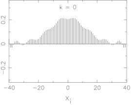
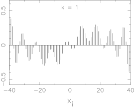
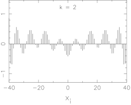
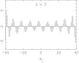
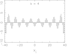
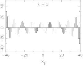
Figure 6: The Gaussian-Hermite dual mode vectors $\tilde{{\textbf{{e}}}}_{k}$ for $k=0,1,\ldots,5$ and $\beta=12$.

3.3 Decomposition of simple functions

Now that we have discussed the properties of the mode vectors and their duals for various values of the scale parameter $\beta$, it is of interest to investigate the effect of taking proper account of linear dependence and non-orthogonal. To this end, we perform the modal decomposition of some simple one-dimensional test functions using both the method advocated in Section 2.1 and the standard approach in which the coefficients in the decompostion are obtained simply by taking scalar products of the image vector with the original mode vectors (see e.g. Refregier 2003). The test functions considered, although simple, are relevant to the decomposition of astronomical images.

Uniform function

We begin by considering the modal decomposition of a uniform signal. The issue of accommodating (nearly) uniform background emission is clearly relevant in an astronomical context. The modal decomposition of this function was calculated, using both the standard method and the SVD method, for $M=20$ modes and for integer values of the scale parameter in the range $\beta=1$–20. In Fig. 7 we plot the resulting decompositions for the standard method (left column) and the approach advocated here (right column) for some representative values of $\beta$.

Figure 7: The uniform function (dashed line) and its modal decomposition (solid line) into $M=20$ Gaussian-Hermite mode vectors with scale parameter $\beta$. The decomposition coefficients are obtained using the standard method (left column) and the SVD method (right column).

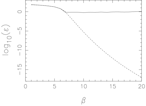
Figure 8: Decomposition residual $\epsilon=|{\textbf{{Ea}}}-{\textbf{{d}}}|$ as a function of $\beta$ for the modal decomposition of the uniform function using the standard method (solid line) and the SVD method (dashed line).

These values have been chosen to correspond to mode sets for which the mode vectors are linearly dependent and non-orthogonal, as demonstrated in Fig. 5. In Fig. 8, we plot the residual $\epsilon=|{\textbf{{Ea}}}-{\textbf{{d}}}|$ of the decompostions as a function of $\beta$ for the standard method (solid line) and the SVD method (dashed line).

We see from Fig. 7 that, as one would expect, the decompositions produced by the two methods differ, in some cases significantly. It was confirmed, however, that for mode sets with $\beta=3$ and $\beta=4$, for which the mode vectors are linearly-independent and orthonormal, the modal decompositions produced by the two methods coincide to machine precision. In the cases illustrated in Fig. 7, we see that the SVD method provides a decomposition that is consistently better than that of obtained with the standard approach. In particular, we note that for a wide range of $\beta$-values, the SVD method produces a decomposition that is visually indistinguishable from the input function, whereas the standard approach exhibits a pronounced ringing for all values of $\beta$. A quantitative description of the improved decomposition quality is given by Fig. 8. As expected, the SVD approach always produces the smallest decomposition residuals, indeed by many orders of magnitude for $\beta\ga 7$. Since the decomposition of an image is a linear process, the ability to describe accurately a uniform function enables better decompositions of discrete objects in a uniform background, which is clearly important in astronomical applications. We also note that, for the SVD method, the decomposition residual is a monotonically decreasing function of the scale parameter $\beta$. For the standard method, however, there is a shallow minimum in the residual at $\beta=7$. It is interesting that, from Fig. 5, for this value of $\beta$ the mode set is neither linearly-independent nor orthogonal.

Top-hat function

As our second illustration, we consider a top-hat function of width equal to 20 units. Once again, this simple function is relevant to astronomical image analysis of, for example, saturated images of compact objects. The modal decomposition of this function was again calculated, using both the standard method and the SVD method, for integer values of the scale parameter in the range $\beta=1$–20. In Fig. 9 we plot the resulting decompositions for the standard method (left column) and the SVD method (right column) for some representative values of $\beta$. The decomposition residuals are plotted in Fig. 10 as a function $\beta$ for the standard method (solid line) and the method (dashed line).

We see from Fig. 9 that, once again, the two methods produce different decompositions for the values of $\beta$ illustrated, and that the SVD method produces superior results. For both methods, however, the presence of only $M=20$ modes leads to considerable ringing in the decompostions for almost all values of $\beta$. Nevertheless, it is interesting that for $\beta=1$ the standard method is unable to produce a reasonable reconstruction, whereas an excellent decomposition is obtained over a limited extent of the function using the SVD method, the extent corresponding to the span of the mode set. The quantitative comparison of the two methods given in Fig. 10 once again shows that, by design, the SVD method always produces the most accurate decomposition. In this case, however, the difference between the two methods is not as great as it was for the decomposition of the uniform function. We also note that the residuals for both methods in this case are minimised at $\beta=3$. At this point, the minimum residual is identical for the two methods, since the original mode set is linear-independent and orthonormal to machine precision.

$\beta$-model profile

Our final one-dimensional illustration is that of a $\beta$-model profile. Clusters of galaxies are often modelled (King 1972) as spherically-symmetric, with an electron density profile of the form

$$n_{\rm e}(r)=n_{0}\left[1+\left(\frac{r}{r_{c}}\right)^{2}\right]^{-3b/2},$$

where $r_{c}$ is the cluster core radius and $b$ is a constant (this is usually denoted by $\beta$, but this has already been used in this paper to denote the scale parameter of the mode set). In this case, one easily finds that the projected thermal Sunyaev-Zel’dovich profile of the cluster is given by

$$f(x)=f_{0}\left(1+\frac{x^{2}}{x_{c}^{2}}\right)^{-\lambda},$$ (10)

where $x$ the angular separation on the sky and $\lambda=(3b-1)/2$. Assuming the standard value $b=2/3$ gives $\lambda=1/2$, and we use this value for our test function, together with a core length $x_{c}=3$.

The modal decomposition of this function was calculated, using both the standard method and the SVD method, for integer values of the scale parameter in the range $\beta=1$–20. In Fig. 11 we plot the resulting decompositions for the standard method (left column) and the SVD method (right column) for some representative values of $\beta$.

Figure 9: As for Fig. 7, but for the top-hat function of width 20.

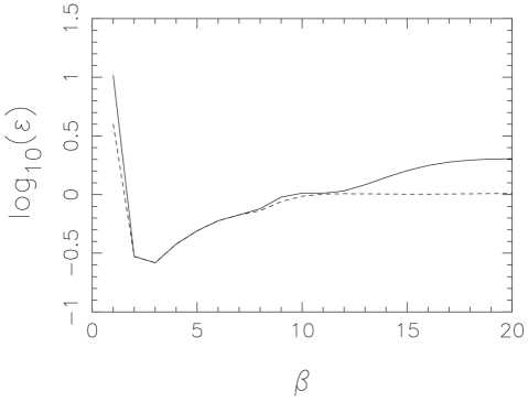
Figure 10: As in Fig. 8, but for the top-hat function of width 20.

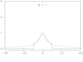
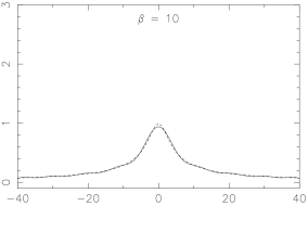
Figure 11: As for Fig. 7, but for the $\beta$-model profile with core radius $x_{c}=3$

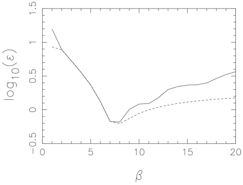
Figure 12: As for Fig. 8, but for the $\beta$-model profile with core radius $x_{c}=3$.

The decomposition residuals are plotted in Fig. 12 as a function $\beta$ for the standard method (solid line) and the SVD method (dashed line).

From Fig. 11, we see again that the SVD methods produces superior decompositions for the values of $\beta$ illustrated. For both methods, some ringing is observed in the decompositions, but this is much less pronounced for the SVD method. In particular, for large values of $\beta$, the standard method cannot accurately reproduce the narrow peak of the $\beta$-model, whereas this is achieved by the SVD method. We also note that, for $\beta=1$, the SVD method reproduces the central sharp peak very accurately. The quantitative comparison of the two methods given in Fig. 11 clearly shows the improvement obtained using the SVD method, which produces a residual significantly below that obtained using the standard method for $\beta\ga 8$. This is also the value of the scale parameter for which both methods yield their lowest residual, and the corresponding set of original mode vectors are close to linearly-dependent and non-orthogonal.

4 Image decompostion

We now consider the modal decomposition of real two-dimensional astronomical images. These images were obtained by first using ${\tt SExtractor}$ (Bertins & Arnouts 1996) on the Hubble Deep Fields (HDFs; Williams et al. 1996, 1998). The convolution mask and detection parameters were adapted from those used by Massey et al. (2003). In particular, in order to allow the recovery of faint objects, we adopted a low signal-to-noise detection threshold, detect_thresh, of 1.3. Objects with class_star $>$ 97 per cent were discarded, since we wish to analyse only galaxies. The image was then segmented into small square ‘postage stamp’ regions around the remaining galaxies. The size of the images were set to $51\times 51$ pixels. In this section, we investigate the decomposition of the HDF galaxy images into a set of two-dimensional Gaussian-Laguerre modes.

4.1 Gauss-Laguerre mode functions

The two-dimensional Gauss-Laguerre continuous mode functions are the simultaneous eigenstates of energy and angular momentum for the two-dimensional isotropic quantum harmonic oscillator. Interestingly, these mode functions are also the solutions in polar coordinates to the paraxial wave equation in optics (see e.g. Goldsmith 1998). The relationship between the standard forms of these mode functions used in the above contexts is discussed in detail in the Appendix.

In the field of optical and quasi-optical systems, it is customary (Murphy et al. 1996; Withington et al. 2000) to define the set of mode functions as

$$\psi_{p}^{m}(r,\theta)=\left[\frac{(2-\delta_{0m})p!}{\pi\beta^{2}(p+|m|)!}\right]^{1/2}x^{|m|/2}\mbox{e}^{-x/2}L_{p}^{|m|}(x)\,\mbox{e}^{\mbox{i}m\theta},$$ (11)

where $x=r^{2}/\beta^{2}$ and $L_{p}^{|m|}(x)$ are the standard associated Laguerre polynomials. The functions $\psi_{p}^{m}$ are conventionally called the Gaussian beam $pm$-modes or simply the $pm$-modes (see e.g. Goldsmith 1998) and form an orthonormal set over the infinite Euclidean plane. The radial index can take the values $p=0,1,2,\ldots,\infty$, and the azimuthal index $m$ can take the values $m=0,\pm 1,\pm 2,\ldots,\pm\infty$. In practice, it is customary to truncate the mode set by imposing maximum values for $p$ and $|m|$. Indeed , it is usual to choose $|m|_{\rm max}=p_{\rm max}$, which leads to a total number of modes ${\cal N}_{1}=(p_{\rm max}+1)(2p_{\rm max}+1)$. If $f(r,\theta)$ is real then clearly $a_{p}^{-m}=(a_{p}^{m})^{*}$.

In the context of quantum mechanics, it is more usual to label the modes in terms of the energy quantum number $n=2p+|m|$ and $m$, rather than $p$ and $m$. Indeed, Refregier (2003) uses this convention to arrive at the polar shapelet modes

$$\phi_{n}^{m}(r,\theta)=\left[\frac{(2-\delta_{0m})({\textstyle\frac{n-|m|}{2}})!}{\pi\beta^{2}({\textstyle\frac{n+|m|}{2}})!}\right]^{1/2}x^{|m|/2}\mbox{e}^{-x/2}L_{\frac{n-|m|}{2}}^{|m|}(x)\,\mbox{e}^{\mbox{i}m\theta},$$ (12)

which also form an orthonormal set over the infinite Euclidean plane. The energy quantum number can take the values $n=0,1,2,\ldots,\infty$, and the azimuthal (angular momentum) quantum number takes the values $m=-n,-n+2,\ldots,n-2,n$, thereby giving $n+1$ values of $m$ for each value of $n$. In practice, one truncates the mode set by imposing a maximum value for $n$, which leads to a total number of modes ${\cal N}_{2}=\frac{1}{2}(n_{\rm max}+1)(n_{\rm max}+2)$. Once again, if $f(r,\theta)$ is real, it is clear that $b_{p}^{-m}=(b_{p}^{m})^{*}$.

4.2 Properties of the mode sets

It is clear from the above discussion (and that given in the Appendix) that the two decompositions (11) and (12) use very different combinations of Gauss-Laguerre modes. The question thus arises as to the relative merits of the two mode sets in decomposing a two-dimensional astronomical image. It is therefore of interest to investigate the properties of pixelised versions of these two mode sets.

As shown by Refregier (2003), by analogy with the criteria (9), the appropriate values of the scale parameter $\beta$ and the maximum energy quantum number $n_{\rm max}$ for the polar shapelet mode set (12) are given by

$$\beta\approx(\theta_{\rm min}\theta_{\rm max})^{1/2},\qquad n_{\rm max}\approx\frac{\theta_{\rm max}}{\theta_{\rm min}}-1$$ (13)

for the decomposition of an image with features on scales ranging from $\theta_{\rm min}$ to $\theta_{\rm max}$. The galaxy images to be decomposed are of size $51\times 51$ pixels, and contain structure down to scales of around 3 pixels. Using the above criteria, we therefore choose $n_{\rm max}=18$. Thus, the total number of polar shapelet modes is 190. To allow a fair comparison between the polar shapelet and $pm$-mode sets, one should arrange for the two sets to contain (as close as possible) the same total number of modes. Fortunately, by choosing $p_{\rm max}=9$, one can arrange for the $pm$-mode set also to contain $190$ modes. The corresponding $pm$-mode and polar shapelet mode vectors are obtained by pixelising the continuous mode functions on the same grid as the galaxy images. Each mode set contains only $190$ modes, which is clearly far less than the number of pixels in the image, but need not be less than the number of degrees of freedom in some class of images. For an arbitrary image of infinite resolution the number of degrees of freedom and pixels will be the same and both decompositions can only represent an approximation to the image.

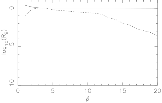
Figure 13: Top: the logarithm of the value of the largest (solid line) and smallest (dashed line) diagonal elements of the Gram matrix ${\textbf{{R}}}={\textbf{{E}}}^{\dagger}{\textbf{{E}}}$ as a function of the scale parameter $\beta$ for the polar shapelet mode set. Middle: the same, but for the $pm$-mode set. Bottom: the logarithm of the largest off-diagonal element of R as a function of $\beta$ for the polar shapelets (dashed line) and $pm$-mode set (solid line).

We may investigate the properties of the polar shapelet and $pm$-mode sets in the same manner as we analysed the one-dimensional shapelet modes. To this end, for each integer value of $\beta$ in the range 0–20, we construct the mode matrix E for both the polar shapelets and $pm$-modes. The rank $r$ of both matrices was found to equal the number of modes (190) for all values of $\beta$ under consideration, hence showing that both modes sets are linearly-independent in all cases. To investigate whether the mode vectors in each set are orthonormal, we calculate the Gram matrix ${\textbf{{R}}}={\textbf{{E}}}^{\dagger}{\textbf{{E}}}$ for each mode set for each value of $\beta$. For an orthonormal mode set R should equal the identity matrix. In Fig. 13 (top and middle), we plot the logarithm of the value of the largest and smallest diagonal element of R for the two mode sets. We see that, for both mode sets, the two curves coincide at $\log(R_{ii})=0$ only for $\beta=3$ and 4, and so it is only for these values of the scale parameter that the mode vectors are of unit length. In the bottom panel of Fig. 13, we plot the logarithm of the largest off-diagonal element of R for the polar shapelet (dashed line) and $pm$-mode set (solid line). We see that, for each mode set, the largest off-diagonal element is only below the machine precision for $\beta=3$, and so it is only for this case that either mode set is orthogonal.

4.3 Decomposition of HDF galaxy images

For the galaxy images to be decomposed, the result (13) suggests one should set $\beta=14$ for the polar shapelets; for comparison purposes we will also use this value of the scale parameter for the $pm$-mode set.

To investigate the relative merits of the two mode sets, we first consider the decomposition of the single galaxy image shown in Fig. 14 (left). In the middle panel, we plot the decomposition residual using the standard approach for the polar shapelets (dashed line) and the $pm$-modes (solid line) as a function of the total number of modes $M$ in the set. As expected, for both mode sets, the decomposition residual decreases as more modes are used. We also see, however, that, for the same total number of modes, the $pm$-modes yield a slightly lower decomposition residual than the polar shapelets. In the right-hand panel of Fig.14, plot the corresponding results obtained using the SVD appraoch. It is clear that, for any given value of $M$, the SVD approach outperforms the standard approach. We also see that, once again, the $pm$-modes yield a lower decomposition residual than the polar shapelets.

The decomposition of five representative galaxy images into the $pm$-mode set are shown in Fig. 15, using both the standard technique (middle column) and the SVD method (right column). As anticipated, since the mode set is not orthogonal, the two decompositions differ, markedly in some cases. For each galaxy image, however, we see that the SVD method produces a more faithful reconstruction. In particular, we note that the SVD method is more successful in reproducing the finer detail of the image. By contrast, the decompositions obtained using the standard approach contain structure only on larger scales. A quantitative comparison of the decomposition quality is given in Table 1, which lists the values of the residual $\epsilon$ of the decomposition. As expected, in each case the SVD method produces a more accurate decomposition than the standard method.

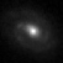
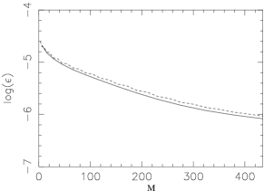
Figure 14: Left: a Hubble Deep Field galaxy. Middle: the decomposition residual using the standard approach for the polar shapelets (dashed line) and the $pm$-mode set (solid line) as a function of the total number of modes $M$ in the set. Right: as middle panel, but using the SVD approach.

5 Discussion and conclusions

We have discussed a general method for performing optimal image decomposition into a set of arbitrary digitised mode functions, which is an everyday problem in astronomy. Our approach may be applied straightforwardly even if the modes are linearly-dependent, non-orthogonal or incomplete, although in the last case the decomposition can only, in general, approximate the original image. By constructing the matrix E containing the digitised modes, the properties of the mode set can be easily obtained by performing a singular value decomposition (SVD). Moreover, having obtained the SVD, the optimal values for the coefficients in the linear decomposition can be obtained immediately. If desired, the optimal coefficients may also be obtained by constructing the set of dual modes, and performing scalar products of these duals with the input data vector. This should be contrasted with the standard method of taking scalar products of the original mode vector with the data vector. This latter approach yields optimal results only in the case where the digitised mode vectors form an orthonormal set. In particular, we note that the digitisation process itself may lead to a mode set that does not inherit the properties of the continuous mode functions from which they are derived. Therefore, considerable care must be exercised when one performs decompositions using digitised versions of continous mode functions that form orthonormal sets. Adopting the standard approach without first investigating the properties of the digitised modes can lead to unnecessarily inaccurate image decompositions.

Image	$\epsilon$ (standard)	$\epsilon$ (SVD)
1	$2.923\times 10^{-3}$	$1.355\times 10^{-3}$
2	$2.688\times 10^{-3}$	$1.938\times 10^{-3}$
3	$1.519\times 10^{-3}$	$1.073\times 10^{-3}$
4	$1.136\times 10^{-3}$	$9.483\times 10^{-4}$
5	$2.235\times 10^{-3}$	$1.165\times 10^{-3}$

Table 1: The residuals $\epsilon$ of the decompositions of the galaxy images shown in Fig.13 for the standard method and the SVD method.

We illustrate our general approach by first applying it to the decomposition of simple one-dimensional functions into Gauss-Hermite (shapelet) modes. We show that, although the continuous shapelet mode functions form an orthonormal set on the entire real line, the corresponding digitised mode vectors can be linearly-dependent and non-orthogonal, depending on the relative values of between the scale parameter $\beta$, the pixel size and the size of the image under analysis. We show that, for a wide range of these values, the method developed here produces decompositions that are significantly superior to those of the standard approach. In some cases, the decomposition residual for our method is many orders of magnitude lower than that for the standard technique.

We also illustrate our method by decomposing images of galaxies extracted from the Hubble Deep Fields into two-dimensional Gauss-Laguerre modes. We consider both the polar shapelet approach where the modes are indexed using the energy and angular momentum quantum numbers $n$ and $m$, and the $pm$-modes used in optics, which are indexed by a radial number $p$ and azimuthal number $m$. In both cases, although the set of continuous functions is orthonormal over the entire Euclidean plane, the correspondinig digitised modes can be severely non-orthogonal, depending on the relative sizes of the mode functions, the image size and the pixel scale. We show that the SVD method proposed here again outperforms the standard approach, yielding more faithful decompositions with lower residuals. We would therefore advise that in future applications of the shapelet decomposition method, the standard approach should be replaced with that presented here. We also find that the $pm$-mode set provides consistently more accurate decompositions than the polar shapelets.

The decompositions presented in this paper used the SVD to provide an optimal decomposition for individual images. Frequently in astronomy, an analysis of the statistics of a collection of images is used to classify astronomical sources and properties. For such an application it may be desirable to use the duals method we have presented. In this case, the set of dual vectors can be calculated using a SVD, without reference to any image. The expansion coefficients for each image can then be very efficiently calculated by performing scalar products with the duals. Additionally, at this stage, a priori knowledge can be used (if desired) to constrain the duals to preferentially extract certain features from any image.

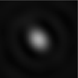
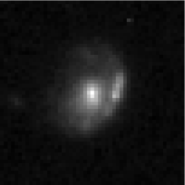
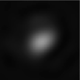
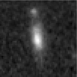
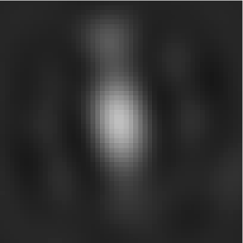
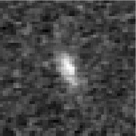
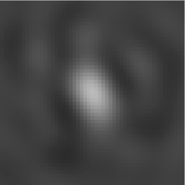
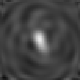
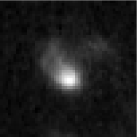
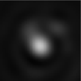
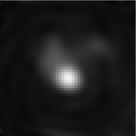
Figure 15: Hubble Deep Field galaxies (left column) decomposed into polar Gauss-Laguerre $pm$-modes with $p_{\rm max}=9$ and $\beta=14$ using the standard method (middle column) and the SVD method (right column).

We conclude that the ability to work straightforwardly with linearly-dependent, non-orthogonal mode sets can be useful not just in accommodating digitisation effects. In many applications, it may be more efficient to work with modes that are known a priori to have such properties. For example, in one or two dimensions, it can be prove useful to decompose images simultaneously in shapelet mode sets centred at a number of points in the image. The ‘multi-centre’ shapelet bases will be discussed in a forthcoming paper. Finally we draw the readers attention to our own previous work investigating generalised bases or arbitrary completeness and orthogonality within the field of THz optics (Berry et al. 2003; Withington et al. 2002), including the description of second-order statistics associated with partially-coherent fields.

ACKNOWLEDGMENTS

RHB acknowledges the support of a PPARC studentship, the Cavendish Laboratory, the Cambridge Philosophical Society and Pembroke College, Cambridge. The authors thank Dr. Phil Marshall for providing the images of HDF galaxies.

Appendix A $pm$-modes and polar shapelets

The Schrödinger equation for the two-dimensional isotropic harmonic oscillator may be written in plane polar coordinates as

$$-{\partial^{2}\psi\over\partial r^{2}}-\frac{1}{r}{\partial\psi\over\partial r}-\frac{1}{r^{2}}{\partial^{2}\psi\over\partial r^{2}}+r^{2}\psi=2E\psi,$$

where we have set $\hbar=m=1$ and chosen our radial coordinate such that the potential is given by $V(r)=\frac{1}{2}r^{2}$. Seeking a separated solution of the form $\psi(r,\theta)=R(r)\Theta(\theta)$, one quickly finds the set of solutions

$$\psi_{p}^{m}(r,\theta)=A\exp(-r^{2}/2)(r^{2})^{|m|/2}L_{p}^{|m|}(r^{2})\exp(\mbox{i}m\theta),$$

where $L_{p}^{|m|}(x)$ is an associated Laguerre polynomial and $A$ is a normalisation constant. In addition to being energy eigenstates, these solutions are clearly also eigenstates of the angular momentum operator $-\mbox{i}\partial/\partial\theta$ with eigenvalue $m$. The angular momentum quantum number may take the values $m=0,\pm 1,\pm 2,\ldots,\pm\infty$, whereas the ‘radial’ quantum number may take the values $p=0,1,2,\ldots,\infty$. Fig. 16 shows the mode function distribution in the $pm$-plane.

Figure 16: The distributions of mode functions in the $pm$-plane. The numbers in brackets denote the value of the energy quantum number $n$ for each mode. The dashed line indicates the usual geometry adopted in the $pm$-plane for truncating the mode set; in this case $p_{\rm max}=|m|_{\rm max}=3$.

Interestingly, the functions (12) are also the solutions of the paraxial wave equation in optics (see e.g. Goldsmith 1998), where they are called the Gaussian beam $pm$-modes or simply $pm$-modes. These modes are often used to describe the electric field distribution in paraxial quasi-optical systems. In this context, it is customary to truncate the mode set by imposing both a $p_{\rm max}$-value and a $|m|_{\rm max}$ value. Moreover, it is usual to choose $|m|_{\rm max}=p_{\rm max}$, so the truncated set of modes form a rectangular in $pm$-space, as illustrated in Fig. 16. In this way, one obtains a total number of modes given by

$${\cal N}_{1}=(p_{\rm max}+1)(2p_{\rm max}+1).$$

It is straightforward to show that the energy of the mode $\psi_{p}^{m}$ is given by (reinstating $\hbar$ for the moment)

$$E=(2p+|m|+1)\hbar\equiv(n+1)\hbar,$$

where $n$ is the energy quantum number. Indeed, in the context of the two-dimensional harmonic oscillator, it is more usual to label the modes in terms of $n$ and $m$, rather than $p$ and $m$. In this way one arrives at the polar shapelet modes

$$\phi_{n}^{m}(r,\theta)=B\exp(-r^{2}/2)(r^{2})^{|m|/2}L_{\frac{n-|m|}{2}}^{|m|}(r^{2})\exp(\mbox{i}m\theta),$$

where $B$ is a normalisation constant. The energy quantum number can take the values $n=0,1,2,\ldots,\infty$, whereas the azimuthal (angular momentum) quantum number takes the values $m=-n,-n+2,\ldots,n-2,n$; hence the energy level with quantum number $n$ is $(n+1)$-fold degenerate. Since we have performed just a simple relabelling, the polar shapelets (12) and the $pm$-modes have the same functional forms, and are directly related by $\psi_{p}^{m}=\phi_{2p+|m|}^{m}$.

Figure 17: The distributions of mode functions in the $nm$-plane. The numbers in brackets denote the value of the radial quantum number $p$ for each mode and indeed may be a more intuitive index than $n$ when investigating images due to $p$ being an intrinisic measure of radial extent and scale. The dashed line indicates the usual geometry adopted in the $nm$-plane for truncating the mode set; in this case $n_{\rm max}=3$.

In Fig. 17 we show the distribution of modes in the $nm$-plane. In Refregier (2003) and Massey et al. (2003), to perform the decomposition of two-dimensional images, the mode set is truncated by imposing an $n_{\rm max}$-value, as illustrated in Fig. 17. In this way, one obtains a total number of modes given by

$${\cal N}_{2}={\textstyle\frac{1}{2}}(n_{\rm max}+1)(n_{\rm max}+2).$$

References

- [] Bertin E., Arnouts S., 1996, A&AS, 117, 393
- [Golub & Van Loan1996] Golub G., van Loan C., 1996, Matrix Computations, John Hopkins University Press, London
- [\citeauthoryearHobson, Jones & LasenbyHobson et al.1999] Hobson M. P., Jones A. W., Lasenby A. N., 1999, MNRAS, 309, 125
- [Massey et al. 2003] Massey R., Refregier A., Conselice C.J., Bacon D.J., 2003, MNRAS, in press (astro-ph/0301449)
- [Press et al. 1994] Press W.H., Teukolsky S.A., Vetterling W.T., Flannery B.P., 1994, Numerical Recipies in Fortran 77, CUP, Cambridge
- [Refregier 2003] Refregier A., 2003, MNRAS, 338, 35
- [Refregier & Bacon 2003] Refregier A., Bacon D., 2003, MNRAS, 338, 48
- [\citeauthoryearSanz, Argüeso, Cayón, Martínez-González, Barreiro & ToffolattiSanz et al.1999a] Sanz J. L., Argüeso F., Cayón L., Martínez-González E., Barreiro R. B., Toffolatti L., 1999, MNRAS, 309, 672
- [\citeauthoryearSanz, Barreiro, Cayón, Martínez-González, Ruiz, Díaz, Argüeso, Silk & ToffolattiSanz et al.1999b] Sanz J. L., Barreiro R. B., Cayón L., Martínez-González E., Ruiz G. A., Díaz F. J., Argüeso F., Silk J., Toffolatti L., 1999, A&AS, 140, 99
- [\citeauthoryearTenorio, Jaffe, Hanany & LineweaverTenorio et al.1999] Tenorio L., Jaffe A. H., Hanany S., Lineweaver C. H., 1999, MNRAS, 310, 823
- [\citeauthoryearWilliams et al.Williams et al.1996] Williams R. et al., 1996, AJ, 112, 1335
- [\citeauthoryearKingKing1972] King I. R., 1972, AJ, 174, 123
- [\citeauthoryear Murphy, J. A. and Withington, S.Murphy, J. A. and Withington1996] Murphy J.A., Withington S., 1996, Infrared Physics and Technology, 37, 205
- [\citeauthoryearWithington, S. and Murphy, J. A. and Yassin, G.Withington, S. and Murphy, J. A. and Yassin, G.2000] Withington S., Murphy J.A., Yassin G., 2000, IEEE Trans. Antennas and Propagation, AP, 49
- [\citeauthoryearWilliams et al.Williams et al.1998] Williams R. et al., 1998, A&AS, 193, 7501
- [\citeauthoryearBerry,R. H. and Withington, S. and Hobson, M.P.Berry2003] Berry R.H., Withington S., Hobson M.P., 2003, JOSA, in press.
- [\citeauthoryearWithington, S. and Berry,R. H. and Hobson, M.P.Withington2003] Withington S., Berry R.H., Hobson M.P., 2003, JOSA, in press.
- [\citeauthoryearBerry,R. H. and Withington, S. and Hobson, M.P. and Yassin,G.Berry2003] Berry R.H., Withington S., Hobson M.P., Yassin G., 2003, in Proc. of Fourteenth International Symposium on Space Terahertz Technology.