Metal Abundances of KISS Galaxies. II.
Nebular Abundances of Twelve Low-Luminosity Emission-Line Galaxies

Abstract

We present follow-up spectra of 39 emission-line galaxies (ELGs) from the KPNO International Spectroscopic Survey (KISS). Many targets were selected as potentially low metallicity systems based on their absolute B magnitudes and the metallicity-luminosity relation. The spectra, obtained with the Lick 3-m telescope, cover the full optical region from [O II]$\lambda\lambda 3726,29$ to beyond [S II]$\lambda\lambda$6717,31 and include measurement of [O III]$\lambda$4363 in twelve objects. The spectra are presented and tables of the strong line ratios are given. For twelve high signal-to-noise ratio spectra, we determine abundance ratios of oxygen, nitrogen, neon, sulfur and argon. We find these galaxies to be metal deficient with three systems approaching O/H of 1/25th solar. We compare the abundance results from the temperature-based T_e method to the results from the strong-line $p_{3}$ method of Pilyguin (2000).

Submitted 22 August 2003; Accepted 29 October 2003 – To appear in the February, 2004 AJ

1 Introduction

Star-forming emission-line galaxies (ELG’s) are important probes of galaxy evolution. Spectra of ELG’s reveal the abundances of heavy elements in the host galaxies (Searle and Sargent 1972; Izotov, Thuan & Lipovetsky 1994; Izotov & Thuan 1999). The measured abundances are tracers of star-formation history and can be used to estimate star-formation rates (Kennicutt 1998, Contini et al. 2002), initial mass functions of the starbursts (Stasinska and Leitherer 1996), and general trends in galactic evolution such as the the metallicity-luminosity relation (Skillman et al. 1989; Richer and McCall 1995; Melbourne and Salzer 2002, hereafter Paper I).

The study of metal abundances of star-forming ELG’s has revealed a class of extremely low-metallicity galaxies such as I Zw 18 and SBS 0335-052, both with metallicities of roughly 1/50th solar (Izotov et al. 1997). In addition to these two extreme galaxies are a handful of galaxies with metallicities roughly 1/25 solar (Izotov et al. 1999). These galaxies are all dwarf systems which follow a metallicity-luminosity trend whereby the less luminous galaxies tend to be less chemically evolved. They place bounds on the primordial composition of the universe, an important observational constraint on Big Bang nucleosynthesis. Izotov et al. (1994, 1997), among others, use these extremely metal-poor systems to infer a value for the primordial helium abundance.

This paper presents spectral follow-up observations of potentially metal-poor systems drawn from the KPNO International Spectroscopic Survey (KISS, Salzer et al 2000). KISS identifies ELG candidates out to a redshift of $z=0.095$ by selecting objects that exhibit line emission in low-dispersion objective-prism spectra. The blue survey (Salzer at el. 2002) identifies objects which possess a strong [O III]$\lambda 5007$ emission feature. The red survey (Salzer et al. 2001, Gronwall et al. 2003) selects objects via the H$\alpha$ line. The sample contains a wide range of star-forming galaxies, such as starburst nucleus galaxies, HII galaxies, irregular galaxies with significant star formation, and blue compact dwarfs. The survey is also sensitive to Seyfert galaxies and quasars with emission lines redshifted into the bandpass of the objective-prism spectra. The red survey, based on the H$\alpha$ selection criterion, remains sensitive to even the most metal-poor ELGs which may be overlooked by surveys with detection criteria based on [O III] lines, blue colors, or UV excess. Therefore we expect that KISS contains several extremely metal-poor systems which will be interesting for abundance studies.

The goals of the current paper are twofold. First, we publish the results of the follow-up spectroscopy obtained over two seasons at the Lick Observatory, as part of the overall effort by members of the KISS group to obtain slit-spectra of KISS ELG candidates. Second, we present the first results of our program to obtain metallicity estimates for potentially low-abundance objects. In Section 2 we discuss the galaxy sample, the observations, and the data-reduction methods. In Section 3 we present the follow-up spectral data obtained at Lick and discuss the properties of the objects observed. Section 4 presents a detailed analysis of the twelve objects with abundance-quality spectra. We measure properties of the nebular emission regions such as electron temperature and electron density and calculate abundance ratios of heavy elements with respect to hydrogen. Section 5 discusses the abundance results, placing them in the context of previous work and exploring the effects of secondary metal production. In addition we we use the sample to examine the recent strong line oxygen abundance methods of Pilyugin (2000, 2001). Our results are summarized in Section 6.

2 Observations and Data Reduction

2.1 Sample Selection

As mentioned above, the galaxies discussed in this paper were chosen from the KISS catalogs primarily as potential metal-poor systems. Observing lists were prepared for each Lick run using the criteria spelled out below. In addition, a number of objects were observed for other purposes entirely. For example, several faint KISS objects with putative radio detections were observed in 2001 as part of a different study (Van Duyne et al. 2003). Hence, the KISS objects for which we present follow-up spectra represent a rather heterogeneous sample, and include a smattering of AGNs and several luminous starburst galaxies in addition to many low-luminosity star-forming systems.

Objects were chosen for follow-up as potential low-metallicity galaxies based on one of two criteria. First, objects with absolute B magnitudes $M_{B}\gtrsim-16$ are found to be metal poor based on the metallicity-luminosity relation (see Paper I). Absolute magnitudes can be derived from the KISS survey data (coarse objective-prism redshifts plus B-band photometry, see Salzer et al. 2000). Based on the published survey data alone, we were able to generate lists of potentially interesting objects using $M_{B}\gtrsim-16$ as our cutoff. Second, follow-up spectra existed for several hundred KISS ELGs at the time these Lick observations were obtained. These were nearly all taken in “quick look” mode, where each object was observed for $\sim$10 minutes or less. For strong-lined ELGs, this is sufficient to obtain an accurate redshift and to assess the nature of the object, even for faint candidates (B = 20 or fainter). However, these short exposures are not adequate for deriving accurate abundances. Also, most of the KISS follow-up spectra have been obtained using spectrographs with no blue sensitivity, meaning that we often do not have data for several important lines, such as [O II]$\lambda\lambda 3726,29$. Therefore, we re-observed several objects at Lick for which their low-metallicity nature had been revealed by certain strong emission-line ratios (e.g., $\mbox{[{O~{}III}]}\lambda 5007/\mbox{H}\beta\;$and [N II]$\lambda 6583/\mbox{H}\alpha\;$) found in their existing follow-up spectra. We were particularly interested in objects for which [O III]$\lambda 4363$ was visible in the “quick look” follow-up spectra. The [O III]$\lambda 4363$/[O III]$\lambda 4959+\lambda 5007$ line ratio is used to measure the nebular electron temperature. Accurate nebular abundance determinations rely on this electron temperature measurement.

In general, these criteria allowed us to identify metal-poor starburst galaxy candidates with a reasonable degree of success. However, in a few cases we discovered high-redshift Seyfert galaxies and quasars rather than low-luminosity starburst galaxies. In some cases a strong [O III]$\lambda$5007 is redshifted to the bandpass covered by the red KISS objective-prism data and is misinterpreted as H$\alpha$ from a low-luminosity, nearby dwarf galaxy. Unfortunately the only way to distinguish these cases is through follow-up spectroscopy, since the objective-prism data are too low resolution to allow one to distinguish between these two options.

2.2 Observations

We obtained spectra of KISS ELGs at the Lick 3-m telescope over the course of three observing runs: April 29, 2000; May 31 - June 1, 2000; and April 27 - 29 2001. The spectra were taken with the KAST double spectrograph which makes use of a dichroic beam splitter (D55) to obtain the full optical spectrum in one observation. We observed with a slit width of 1.5 arcsec and used Grating 2 (600/7500) on the red side giving a reciprocal dispersion of 2.32 Å/pixel and Grism 2 (600/4310) on the blue side giving a reciprocal dispersion of 1.85 Å/pixel. The full spectral range provided by this setup was from 3500 Å to 7800 Å. Exposure times ranged from 20 minutes to 80 minutes (see below), with the longer observations taken in 20 minute increments and combined later. Each night of observations included spectra of a Hg-Cd-Ne and Ne-Ar lamps to set the wavelength scale as well as several spectrophotometric standard stars for flux calibration.

Our brighter targets were visible directly on the slit-viewing camera available for the KAST spectrograph. However, for fainter objects (roughly B $>$ 17) we could not see the sources clearly in the camera, and were forced to use the following procedure. We removed the grating and opened the slit jaws, then took a short exposure image of the source. We then moved the telescope until the target was centered on the known location of the narrowed slit. While somewhat inefficient, this procedure allowed us to position even extremely faint objects in the slit of the spectrograph. The faintest object we observed had a B magnitude of 21.24. The slit orientation was fixed at a position angle of 90^∘ (E-W), to minimize the effect of differential atmospheric refraction for our sample of targets, which have declinations comparable to the latitude of the observatory.

The amount of integration time each object received varied depending on the nature of the source. For objects without previous follow-up spectra, it was unclear whether obtaining a high S/N abundance-quality spectrum was warranted. After obtaining a preliminary exposure of $\sim$20 minutes, the resulting spectrum was evaluated in real time. Objects that were found to contain the auroral [O III]$\lambda 4363$ line of sufficient strength to yield a high quality abundance were then observed for additional time. In this way high signal-to-noise spectra were taken only for the most promising low-metallicity candidates. Objects whose spectra did not contain the [O III]$\lambda 4363$ line were only observed for the single exposure. In nearly all cases, these data are sufficient for determining fundamental properties about the galaxies, such as redshift, galaxy activity type, and values for the strong emission-line ratios.

2.3 Data Reduction

The data reduction was carried out with the Image Reduction and Analysis Facility (IRAF). Processing of the 2D spectral images followed standard methods. All of the reduction steps mentioned below were carried out on the red and blue spectral images independently. The mean bias level was determined and subtracted from each image by the data acquisition software automatically. A mean bias image was created by combining 15 zero-second exposures taken on each night. This image was subtracted to correct the science images for any possible 2D structure in the bias frames. Flat fielding was achieved using an average-combined quartz-lamp image that was corrected for any wavelength-dependent response.

1D spectra were extracted using the IRAF APALL routine. The extraction width (i.e., distance along the slit) was selected independently for each source by examination. For most sources the emission region was unresolved spatially, so that the extraction width was limited to $\sim$5-6 arcsec. Sky subtraction was also performed at this stage, with the sky spectrum being measured in 8-12 arcsec wide regions on either side of the object window. The Hg-Cd-Ne and Ne-Ar lamp spectra were used to assign a wavelength scale, and the spectra of the spectrophotometric standard stars were used to establish the flux scale. The standard star data were also used to correct the spectra of our target ELGs for telluric absorption. This is important because a number of our ELGs are at redshifts where the [S II] doublet falls in the strong B-band and would otherwise lead to a severe underestimate of the true line flux. The emission-line fluxes and equivalent widths were measured using the SPLOT routine. When multiple images of the same object were available, the spectra were reduced separately then combined into a single high S/N spectrum prior to the measurement stage.

The KAST spectrograph uses a dichroic beam splitter to break the spectrum into red and blue sections. In order to analyze the data it is necessary to ensure that the red and blue regions are on a consistent flux scale. To achieve this, we made certain that the extraction regions used in APALL were precisely the same for both the red and the blue sections. We utilize the standard star observations to measure any remaining small-scale shifts between the red and blue sides. To do this, we measured the flux in the continua of the standard stars taken each night in 100 Å bins from 5000 Å to 5800 Å. A plot of flux vs. wavelength reveals any small shifts between the continuum fluxes on either side of the dichroic break. Since the image scales for the red and blue sides are the same, and since the same spectral extraction regions were used for both sides, the correction factors were expected to be small. This turned out to be the case, with the derived correction factors for each night of observations ranging from a few percent up to 10 - 12%. For our instrumental setup, H$\alpha$ and H$\beta$ are nearly always on opposite sides of the dichroic. Therefore the main effect of the correction factor is to modify the H$\alpha$/H$\beta$ ratio, and hence the measured value of $c_{H\beta}$ (see below). Thus, this necessary procedure introduces an additional level of uncertainty into the derivation of the nebular abundances (Section 4) in the sense that it affects the reddening corrections.

For an initial estimate of the internal reddening in each galaxy we calculate $c_{H\beta}$ from the H$\alpha$/H$\beta$ line ratio. $c_{H\beta}$ is then used to correct the measured line ratios for reddening, following the standard prescription (e.g., Osterbrock(1989):

$$\frac{I(\lambda)}{I(\mbox{H}\beta)}=\frac{F(\lambda)}{F(\mbox{H}\beta)}exp[c_{H\beta}f(\lambda)]$$ (1)

where f($\lambda$) is derived from studies of absorption in the Milky Way (using values taken from Rayo et al. 1982). Estimates of $c_{H\beta}$ for each galaxy are given in Tables 1-3. A more rigorous estimate of $c_{H\beta}$ is made for the abundance-quality spectra (Section 4.1, Table 6).

3 The Spectral Data

=5.0in

Figure 1: Representative spectra of KISS objects obtained with the KAST spectrograph on the Lick Observatory 3-m telescope. a) The starburst galaxy KISSR 1021. b) The QSO KISSR 1332, which is detected by KISS via the strong [O III] line. c) The LINER KISSR 1412. d) The high redshift Seyfert 2 galaxy KISSR 1751, for which the [O III] lines are shifted into the bandpass of the red KISS filter. The red and blue sides of these spectra have different dispersions. Therefore line ratios between lines from the two sides should not be compared using this Figure. The flux scales on the red and blues sides were carefully calibrated (see Section 2.3).

The results of our spectroscopic observations of the Lick Sample are presented in Tables 1 - 3. The tables are organized by the source KISS catalogs in which the targets are located. Table 1 lists the results for KISS ELGS from the first red survey list (30^∘ Red Survey; Salzer et al. 2001), Table 2 presents the spectral data for objects from the second red survey list (43^∘ Red Survey; Gronwall et al. 2003), and Table 3 gives the data for the blue survey list (30^∘ Blue Survey; Salzer et al. 2002). All three tables have precisely the same format. Column 1 gives the KISS number from the relevant catalog, while columns 2 & 3 list the survey field and ID number designation. Column 4 indicates the observing run during with the spectrum was obtained. The values represent specific dates from the various runs: 81 = 29 April 2000, 82 = 31 May 2000, 83 = 1 June 2000, 161 = 27 April 2001, and 163 = 29 April 2001. Column 5 lists a coarse spectral quality code. Q = 1 refers to high quality spectra, with high S/N emission lines and reliable emission-line ratios. Q = 2 is assigned to objects with lesser quality spectra but still reliable line ratios. Q = 3 refers to spectra where the data are of low quality, usually due to the faintness of the object and/or the weakness of the emission lines. Column 6 lists the redshift, obtained from the average of the redshifts derived from all of the strong emission lines. Typical formal uncertainties for z are 0.00005 - 0.00010 (15 - 30 km/s). Column 7 gives the decimal reddening coefficient c_Hβ, which is defined in equation 1. In several cases the derived values for c_Hβ are negative. In virtually all instances where this occurs, the formal error in c_Hβ is such that the measured value is consistent with c_Hβ = 0.00. Whenever a negative c_Hβ is measured, we adopt c_Hβ = 0.00 for the computation of reddening-corrected line ratios.

=5.0in

Figure 2: A plot of log$(\mbox{[{O~{}III}]}\lambda 5007/\mbox{H}\beta)$ as a function of log$(\mbox{[{N~{}II}]}\lambda 6583/\mbox{H}\alpha)$ for objects classified as starbursting types in the KISS database. The filled symbols are objects that have follow-up spectra in the KISS database of quality code 1 or 2. The open diamonds represent the objects observed with the Lick 3m.

Columns 8 through 11 of the data tables present the observed equivalent widths of [O II]$\lambda\lambda$3726,29, H$\beta$, [O III]$\lambda$5007, and H$\alpha$. Column 12 lists the H$\alpha$ flux, in units of 10^-16 ergs s^-1 cm^-2. These values should be treated with caution, since the conditions during the observing runs were not always photometric, and the seeing was highly variable. Columns 13 - 16 give the logarithms of the reddening-corrected line ratios for log$(\mbox{[{O~{}II}]}\lambda\lambda 3726,29/\mbox{H}\beta)$, log$(\mbox{[{O~{}III}]}\lambda 5007/\mbox{H}\beta)$, log$(\mbox{[{N~{}II}]}\lambda 6583/\mbox{H}\alpha)$, and log([S II]$\lambda\lambda$6717,31/H$\alpha$) for each galaxy. If an equivalent width or line ratio measurement is not listed, either the relevant line was not present in the spectrum (often due to low S/N), or the line is redshifted out of the region covered by our spectra. The latter is true for lines like [N II]$\lambda\lambda$6548,83, H$\alpha$, and [S II]$\lambda\lambda$6717,31 in the several objects with z $>$ 0.3. Finally, Column 17 indicates the activity type for each object: SBG = Starburst Galaxy (i.e., any type of star-forming ELG), SY2 = Seyfert 2, LIN = low-ionization nuclear emission region (LINER), QSO = quasi-stellar object, Gal = non-emission-line galaxy, Star = Galactic star. The latter two categories represent objects that are not actually extragalactic emission-line sources, and hence are objects mistakenly identified by the survey as ELGs. To date, follow-up spectroscopy has shown that $\sim 8-9$% of the objects cataloged in KISS are actually non-ELGs.

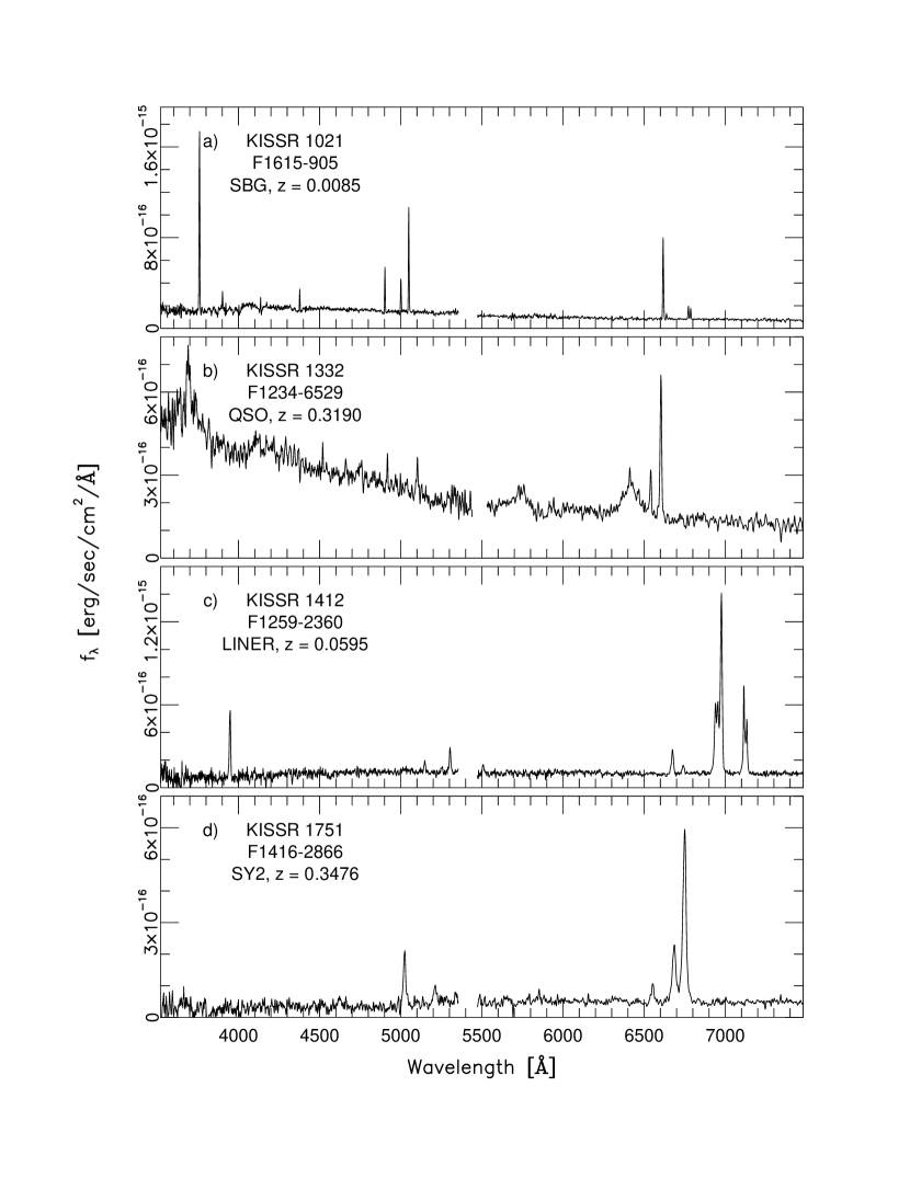
Characteristic spectra of objects observed with the Lick 3-m telescope are presented in Figure 1. These were selected to illustrate the range of objects identified by KISS. Shown are the spectra of a low redshift star-forming galaxy (Figure 1a), a moderate redshift QSO (Figure 1b), a LINER (Figure 1c), and a moderate redshift Seyfert 2 galaxy (Figure 1d). Both the QSO and the Seyfert 2 are examples of objects selected from the red survey (H$\alpha$-selected) where another emission line ([O III]$\lambda 5007$ in both cases) is redshifted into the low-z H$\alpha$ region. About 2% of the KISS galaxies with follow-up spectra fall in this category; most are AGNs. A more complete discussion of the AGN population found in the KISS catalogs is given in Gronwall, Sarajedini & Salzer (2002) and Stevenson et al. (2003). The spectra of the 12 objects for which nebular abundances are derived are shown in the following section.

In Figure 2 we present a diagnostic diagram (e.g., Baldwin, Phillips & Terlevich 1981; Veilleux & Osterbrock 1987) plotting log$(\mbox{[{O~{}III}]}\lambda 5007/\mbox{H}\beta)$  against log$(\mbox{[{N~{}II}]}\lambda 6583/\mbox{H}\alpha)$  for all KISS objects with follow-up spectra of quality code Q = 1 or 2 which are classified as star-forming types (points). The galaxies observed at Lick are shown as diamonds. Different types of star-forming galaxies are located in different regions of the plot. Low metallicity starbursts are found in the upper left. High metallicity starbursts are located in the lower right. AGN and LINERS are found in the upper right portion of the diagram. Only one of the AGNs observed at Lick has the relevant emission-line ratios necessary to be plotted in Figure 2 (KISSR 1412, a LINER). It falls off the diagram, to the right. All of the other AGNs are high redshift objects that lack the [N II]$\lambda$6583/H$\alpha$ ratio. Note that most of the objects in the Lick sample are located in the upper left section of the diagram, suggesting that they are metal-poor objects. This is exactly what one would expect given the selection criteria.

Of the 39 objects in our sample, 29 are classified as starburst/star-forming galaxies of some type, three are Seyfert 2s, one is a LINER, one is a QSO. Five objects are non-ELGs: two are Galactic stars and three are galaxies with no emission lines. A more complete discussion of the spectroscopic properties of these galaxies will be presented in a future paper summarizing the spectroscopic follow-up of the entire KISS sample.

4 Metal Abundances

Twelve galaxies in our sample were observed with a high enough signal-to-noise ratio to detect [O III]$\lambda 4363$. The [O III]$\lambda 4363$ line provides a measure of the electron temperature in the star-forming regions of these galaxies. Using the temperature in conjunction with the measured line ratios we calculate accurate metal abundances.

General properties of the sample are given in Table 4. Column 1 gives the KISSR/KISSB number of the object. Column 2 shows the apparent $B$ magnitudes which range from 15.6 to 19.9. The median m_B is 17.6, and the sample contains three galaxies with $m_{B}>19.5$, significantly fainter than most objects found in traditional nebular abundance studies. Column 3 gives the $B-V$ color of each galaxy corrected for Galactic reddening. Column 4 shows the absolute $B$ magnitude of each galaxy. $M_{B}$ varies from -12.5 to -17.5, and thus tends to be on the fainter end of the KISS ELG luminosity distribution. This is not surprising since we were targeting objects that were expected to have low metallicity. Column 5 gives the recessional velocity in km/sec, and Column 6 gives the calculated metallicity of the object (see Sections 4.1 - 4.3). Overall the sample galaxies tend to be fainter and more distant than the galaxies studied by previous groups doing nebular abundances. While this makes it more difficult to do accurate abundance work, we find that reasonable results are possible. Not surprisingly, the formal errors in our final abundance estimates tend to be somewhat higher than those obtained in many of these previous studies. However, the precision of our results is still adequate for most applications to the statistical study of chemical evolution in galaxies.

The following section details the metal abundance determinations. We will refer to the temperature-based abundance determination as the T_e method.

4.1 The Spectra and Line Ratios

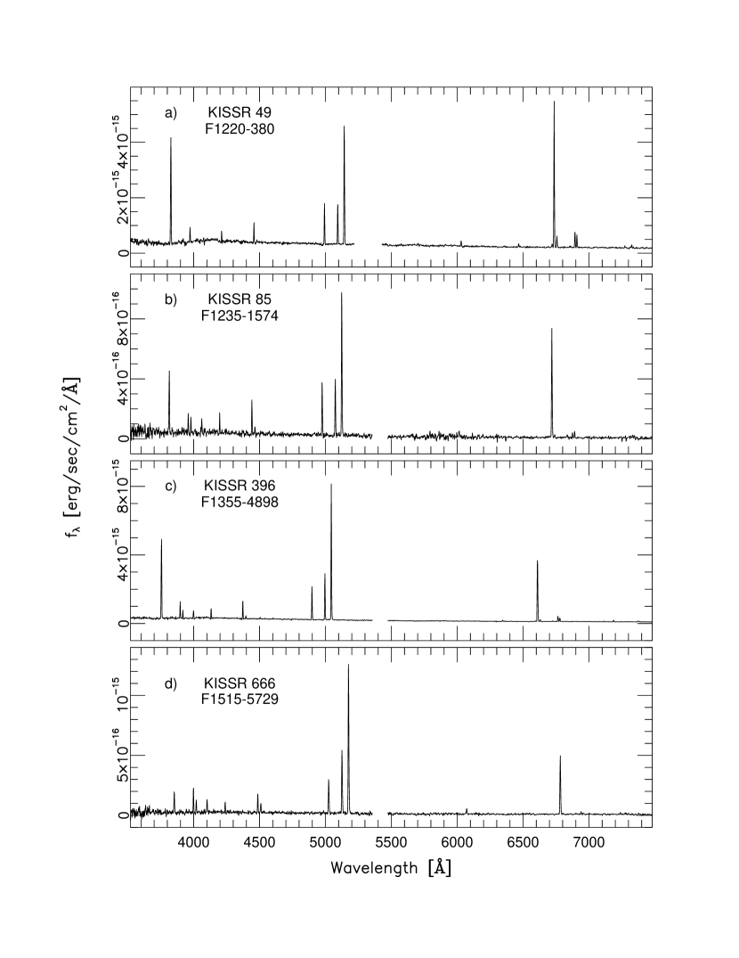
The spectra of our 12 abundance-quality objects are presented in Figure 3. These sources are characterized by low continuum emission with very strong emission features. These spectra generally have a high log$(\mbox{[{O~{}III}]}\lambda 5007/\mbox{H}\beta)$  ratio and a low log$(\mbox{[{N~{}II}]}\lambda 6583/\mbox{H}\alpha)$ ratio indicative of low metal abundance and high excitation star-forming regions. The spectra also contain detections of sulfur, neon, argon, and helium lines. Measurements are made of all the lines with equivalent width exceeding 1 Å. Raw and reddening-corrected line ratios are presented in Tables 5 and 6, respectively.

=5.0in

Figure 3: Plots of the 12 abundance-quality spectra obtained with the Lick Observatory 3-m telescope. As with Figure 1, the red and blue sides of these spectra have different dispersions. Therefore line ratios between lines from the two sides should not be compared using this Figure. Specifically, the apparent H$\alpha$/H$\beta$ line ratios will not be correct in this Figure.

=5.0in

=5.0in

The $c_{H\beta}$ values used for the reddening correction were determined from a simultaneous fit to the reddening and absorption in the Balmer lines, using all available Balmer line ratios. The stellar absorption, usually not exceeding 3 Å of equivalent width, is corrected for, and a value for $c_{H\beta}$ is obtained for each galaxy by using the average of the values for the three highest-order Balmer line ratios. Because KAST is a dual channel spectrograph there is the added complication of putting the red and blue sides on the same flux scale. In certain cases this caused problems with determining an accurate value for $c_{H\beta}$. However, we posses additional spectra of these objects that cover the full optical range in one image. We use these additional spectra to confirm and in some cases revise the H$\alpha$/H$\beta$ line ratio used to infer the reddening corrections. The adopted values of $c_{H\beta}$ are given in Table 6. (Note: these values are different than the estimated $c_{H\beta}$ values given in Tables 1-3.)

Four of the twelve galaxies have been observed spectroscopically by other groups. KISSR 49, also known as CG 177, was observed by Salzer et al. (1995) as part of a follow-up of Case ELGs. The uncorrected[O II]/H$\beta$ and [O III]/H$\beta$ line ratios from the two studies match within the errors. KISSR 396, also known as Was 81, was first observed by Wasilewski (1983) using a SIT vidicon spectrograph. He measured [O III]/H$\beta=2.8$, while we find [O III]/H$\beta=4.1\pm 0.1$. A confirming spectrum from the Michigan-Dartmouth-MIT (MDM) 2.4-m telescope (Wegner et al. 2003) agrees with all the major Lick line ratios to within the errors, indicating that the more recent results are reliable. KISSR 1752, the extremely metal-poor object SBS 1415+437 was observed by Thuan et al. (1999). The high signal-to-noise-ratio observations taken by Thuan et al. are equivalent to the Lick results to within errors for all the major indices. Finally KISSR 1845, also known as CG 903 and HS 1440+4302 was observed by Popescu & Hopp (2000) in a survey of dwarf galaxies in voids and by Ugryumov et al. (1998, 1999). In this case we find agreement with Popescu et al. to within the errors for the strong [O III]/H$\beta$ line ratio. However, they find [O II]/H$\beta=5.30$ while we find [O II]/H$\beta=2.43$. Some of this difference can be accounted for by discrepant $c_{H\beta}$ measurements. We found $c_{H\beta}=0.113$ while they found $c_{H\beta}=0.336$. The additional discrepancy is probably due to the flux calibration at the blue end of the spectrum which tends to be difficult to do consistently, or to the significant difference in slit width used by the the two studies (1.5″ for our study, 4″ for Popescu). In summary, our [O III]/H$\beta$ line ratios compare well with previous studies while in one case the [O II]/H$\beta$ ratios vary significantly.

4.2 Electron Density and Temperature

We assume a two zone model for the star-forming nebula, a medium-temperature zone where oxygen tends to be doubly ionized and and low-temperature zone where oxygen is singly ionized. Within the radius of the low-temperature zone hydrogen is ionized and beyond this zone hydrogen is assumed to be neutral.

Ideally we would like to know the electron density and temperature in each zone. However, the data available only allow for an electron density measurement in the low-temperature zone, and an electron temperature measurement in the medium-temperature zone. We use the [S II]$\lambda$6716/$\lambda$6731 (Izotov et al. 1994) ratio to determine the electron density, which in all measurable cases is roughly 100 e^-cm^-3. In several cases the sulfur lines are too noisy to accurately determine the electron density. In half of these cases the [S II]$\lambda$6716/$\lambda$6731 doublet falls within the atmospheric B-band. For galaxies where electron density was not calculated, we assume a density of 100 e^-cm^-3. In all cases we assume that the density does not vary significantly from zone to zone. The electron temperature in the medium temperature zone is given by the oxygen line ratio [O III] ($\lambda 4959+\lambda 5007$)/$\lambda$4363 (Izotov et al. 1994). Calculations of both the electron density and electron temperature are carried out using the IRAF NEBULAR package (Shaw & Dufour 1995), which makes use of the latest collision strengths and radiative transition probabilities.

We estimate the temperature in the low-temperature zone by using the algorithm presented in Skillman et al. (1994) based on nebular models of Stasinska (1990)

$$t_{e}(OII)=2((t_{e}(OIII)^{-1}+0.8)^{-1},$$ (2)

where t’s are temperatures measured in units of $10^{4}$ K. The measured electron densities and temperatures are presented in Table 7.

Metal abundance measurements depend critically on a knowledge of the nebular electron temperature. However, the [O III] $\lambda$4363 is often weak and for two objects in our sample it is suspect. These cases and the solutions adopted are discussed below.

The spectrum of KISSR 666 gives an unusually high electron temperature, over 20,000 K. However, the [O III] $\lambda$4363 lines in the individual Lick spectra (that were summed to produce the final spectrum) appear noisy. This is not surprising since the galaxy is very faint with $m_{B}=19.81$, much fainter than galaxies traditionally studied for abundances. In order to confirm this unusual result, we decided to re-observe the object with the Monolithic Mirror Telescope (MMT). The larger aperture of the MMT allowed for a cleaner spectrum which indicated a significantly lower electron temperature of 16,500 K. Because the spectrum from the MMT had a higher signal-to-noise ratio, we adopted that temperature (Lee et al. 2004) for the subsequent abundance analysis of the Lick spectrum.

In a similar case, the spectrum of KISSB 23 appears to have a suspect [O III] $\lambda$4363 line. The line observed in our Lick spectrum is unphysically broad. This odd shape is repeated in all four of the individual spectra. In addition, the center of the putative [O III] $\lambda$4363 line is offset slightly in wavelength compared to its expected position. We re-observed this object on the MMT as well. The MMT spectrum does not reproduce the odd shape of the line, indicating that the Lick spectrum is suspect. We hypothesize that scattered light in the KAST spectrograph fell upon the location of the [O III] $\lambda$4363 line giving it the observed broad appearance and leading to an over-estimation of the line flux. We again adopt the temperature calculated from the MMT spectrum (14750 K, Lee et al. 2004).

4.3 Calculating Metal Abundances

We use the IRAF NEBULAR package (Shaw & Dufour 1995) to calculate ionic abundances relative to hydrogen. The input data tables include the densities and temperatures of each ionization zone, as calculated above, and the emission-line ratios measured previously (Table 6). We calculate the abundance of the following ions with respect to H⁺: O⁺, O⁺⁺, N⁺, S⁺, S⁺⁺, Ne⁺⁺, and Ar⁺⁺.

Ionization correction factors account for the additional ionization states present in the nebula that do not emit in the optical spectrum. We use the prescription of Izotov et al. (1994) given by:

$$ICF(N) = \frac{N}{N^{+}}=\frac{O}{O^{+}},$$ (3)

$$ICF(Ne) = \frac{Ne}{Ne^{++}}=\frac{O}{O^{++}},$$ (4)

$$ICF(S) = \frac{S}{S^{+}+S^{++}}$$ (5)

$$= [0.013+x\{5.10+x[-12.78+x(14.77-6.11x)]\}]^{-1},$$

$$ICF(Ar) = \frac{Ar}{Ar^{++}}$$ (6)

$$= [0.15+x(2.39-2.64x)]^{-1},$$

$$x = \frac{O^{+}}{O}.$$ (7)

In addition Izotov et al. offer a calculation for O⁺⁺⁺ given by:

$$\frac{O^{+++}}{O^{++}}=\frac{He^{++}}{He^{+}}.$$ (8)

However, in the few cases where we observe He⁺⁺ in the spectra, the line is very noisy and we assume that the amount of O⁺⁺⁺ in the nebulae is negligible.

Using the ionic abundances and ionization correction factors given above, we deduce the O/H, N/H, and Ne/H ratios for each galaxy. Measurements of the sulfur abundance ratios, S/H are limited to the 6 galaxies in which we measure S⁺⁺. We measure Ar/H in 8 of 12 galaxies. The abundance results are presented in Table 7. (Note: preliminary metallicities for this sample of galaxies were presented in Paper 1. The metallicities reported here are updated and supersede the preliminary results. We plan to use the final results from this paper, in conjunction with metallicity results from Lee et al. (2004) to update the metallicity – line-ratio relationships given in Paper 1.)

We generate error estimates for the abundance data in Table 7 in the following way. We use the one sigma errors in the oxygen line ratios to generate new T_e[OIII]_dev measurements for each system. The error in the electron temperature is then given by,

$$\sigma(T_{e}[OIII])=T_{e}[OIII]-T_{e}[OIII]_{dev}$$ (9)

We then propagate this error estimate through equation 2 to obtain $\sigma(T_{e}[OII])$. We run the abundance programs with temperature offsets to generate a second abundance estimate for each element. We take the difference between the original ionic abundance estimate and the new estimate as the error in the ionic abundance. In order to account for the effects of errors in the observed line ratios, we add in quadrature the percentage error of the line ratio to the temperature-based error for each ion. Errors in temperature range from 10% to 4% and result in final metallicity errors of 0.04 – 0.09 dex. A comparison of our metallicity result for the extremely metal-deficient KISSR 1752 with Thuan et al. (1999) reveals good agreement. We find 12 + log(O/H)$=7.57\pm 0.04$ while they give $7.60\pm 0.01$. In addition, for the three galaxies where we have an independent MMT spectrum we find good agreement in the metal abundances derived from the two spectra.

5 Discussion of Metallicity Results

5.1 Abundances and Abundance Ratios

The final abundance estimates are given in Table 7. It is standard to refer to the metallicity of a galaxy in units of 12 + log(O/H). In these units solar metallicity is 8.92 (Lambert 1978). (A more recent determination of the solar oxygen abundance by Allende Prieto et al. (2001) gives a metallicity of 8.69. We will however continue to refer to the older solar abundance value so that we can more easily compare with previous work.)

We find that all twelve galaxies studied here are metal poor with 12 $+$ log(O/H) $<$ 8.1. The mean metallicty of the sample is 7.79 (1/13th solar), and three galaxies are extremely metal deficient, approaching 12 $+$ log(O/H) $\sim$7.5, or $\sim 1/25$ solar. As mentioned above, the formal errors on our abundances are somewhat higher than many previous studies, due to the faintness of many of our sources. The average error in the oxygen abundance is 0.056 dex, and in all cases the errors are smaller than 0.1 dex.

=5.0in

Figure 4: Abundance ratios as a function of metallicity are plotted for Lick data (diamonds) and the Izotov and Thuan (1999) dataset (points). Panel (a) shows the neon to oxygen ratio, panel (b) is the sulfur to oxygen ratio, while panel (c) is the nitrogen to oxygen ratio. Typical error bars for the Izotov and Thuan data are shown in the lower right of each plot.

Metal enrichment of galaxies occurs as a result of at least two processes, ejection of enriched material during core collapse and type Ia supernova, and matter loss through stellar winds. The $\alpha$ elements such as oxygen, sulfur, neon and argon are produced in massive stars. Because they are created under the same conditions, the ratio of these elements should remain constant with increasing O/H ratios. This has been demonstrated empirically in Izotov and Thuan (1999), among others. Panel (a) of Figure 4 shows the Ne/O ratio as a function of O/H for the Lick data (diamonds) and the Izotov and Thuan dataset (points). Panel (b) shows S/O. In general the Lick data agree with the Izotov and Thuan data, albeit with a somewhat higher scatter. We find the mean log(Ne/O) $=-0.65\pm 0.07$ while Izotov and Thuan gives log(Ne/O) $=-0.72\pm 0.06$. Similarly for sulfur we find a mean log(S/O) $=-1.47\pm 0.14$ with Izotov and Thuan reporting log(S/O) $=-1.56\pm 0.06$. Argon (not plotted) has similar behavior to neon and sulfur. We find a mean log(Ar/O) $=-2.20\pm 0.13$, while Izotov and Thuan give mean log(Ar/O) $=-2.26\pm 0.09$.

The production of nitrogen is more complicated than the $\alpha$ elements because nitrogen production can be enhanced by the CNO cycle in lower mass stars. However, for low metallicity galaxies it has been found that N/O is constant for increasing O/H (Izotov and Thuan 1999). In panel (c) of Figure 4 we plot the N/O ratio as a function of O/H again comparing the Lick data (diamonds) to the Izotov and Thuan data (points). The Lick data give a mean log(N/O) $=-1.42\pm 0.12$ while Izotov and Thuan give log(N/O) $=-1.47\pm 0.14$. No significant nitrogen enhancements are noticeable in the figure, and we concur with van Zee et al. (1998) and Izotov & Thuan (1999) that nitrogen is a primary element in low metallicity systems and only becomes significantly enhanced with respect to oxygen at metallicities higher than that of the galaxies contained in the Lick sample.

Helium abundances, especially in low metallicity systems like the ones being studied here, are exciting to measure because they can place bounds on the primordial helium abundance. While helium lines were detected in all twelve spectra, they were not high enough signal-to-noise to allow for a reasonably accurate determination of the helium abundance. Higher quality spectra of these objects may prove interesting for future studies of helium abundances in low-metallicity systems.

5.2 T_e vs. $p_{3}$ Metallicities

=4.0in

Figure 5: A comparison of metal abundances calculated with T_e and $p_{3}$ methods. The difference between the two methods is plotted against the factional error in the temperature measurement.

Because the T_e metal abundances are so dependent on the quality of the [O III]$\lambda 4363$ line, we compare the T_e abundance results with metallicities derived from the strong oxygen lines alone. Recently, Pilyugin (2000, 2001) demonstrated a method for calculating metallicity from the strong oxygen lines [O II]$\lambda\lambda 3726,29$ and [O III]$\lambda\lambda 4959,5007$. The Pilyugin method (hereafter the $p_{3}$ method) is an empirical result that relates ratios of the strong oxygen lines and H$\beta$ with metallicities measured with the T_e method. He finds that his method agrees with the T_e method to within 0.1 dex for low metallicity systems. In fact he suggests that his method can be more accurate than the T_e method when the [O III]$\lambda$4363 line is weak (Pilyugin 2001). This claim is based partly on data from the Hidalgo-Gamez and Oloffson (1998) metallicity-luminosity work. Hidalgo-Gamez and Oloffson found little evidence for a metallicity-luminosity relation in their sample of starbursting galaxies, where metallicity was measured with the T_e method. When the metallicities were recalculated using the Pilyugin method, the data closely follow the Skillman et al. (1989) metallicity-luminosity relation. This may indicate that the T_e method is less reliable than the strong line method when [O III]$\lambda$4363 is noisy.

=5.0in

Figure 6: A metallicity-luminosity relation. The diamonds are data from this paper with metallicity calculated by the T_e method. The triangles are data from Skillman et al. (1989). The dashed line is the fit to the Skillman et al. data.

=5.0in

Figure 7: The same as Figure 6, except that the metallicity for the Lick objects is now calculated with the $p_{3}$ method.

We use the $p_{3}$ method to generate a second metallicity estimate for our galaxies. The results are included in Table 7. We find that nine of the twelve galaxies have $p_{3}$ abundances within 0.1 dex of their T_e result. The other three are within 0.2 dex. In order to illustrate this result, we plot the difference between the T_e and $p_{3}$ metallicity results vs $\sigma$(T${}_{e})/$T_e in Figure 5. We see that all three deviant galaxies have $\sigma$(T${}_{e})/$T${}_{e}>0.07$ and tend to be noisier spectra.

One of our most deviant objects is KISSB 23, which gives a $p_{3}$ metallicity 0.17 dex higher than its $T_{e}$ result. What is interesting in this case is that the excitation indicator [O III]$\lambda$5007/[O II]$\lambda\lambda$3726,29 appears to be quite low, suggesting that this object may be past the peak of its starburst phase, with the most massive stars already evolved off the main sequence. Objects like this are rare in most ELG surveys, since post-peak objects are often fainter and have weaker emission lines. We have, however, found a similar object in the Skillman et al. (1989) dataset. Sextans A field 1 has a low excitation index but a high temperature and low metallicity. When we calculate a $p_{3}$ abundance for this object we find that $p_{3}$ gives an abundance 0.3 dex higher than the $T_{e}$ method. This may be suggesting that $p_{3}$, which has been calibrated with a dataset composed exclusively of high excitation objects, is not reliable for objects with lower excitation spectra.

To further investigate whether $p_{3}$ or T_e is more reliable, we use Pilyugin’s idea of looking for a tight metallicity-luminosity relation. In Figure 6, we plot T_e abundances for our galaxies as filled diamonds. For comparison, we include the Skillman et al. (1989) data shown as triangles. The fit to the Skillman data is shown as a dashed line. In Figure 7 we plot the same, using our $p_{3}$ metallicities. We see that both the T_e and $p_{3}$ results appear to mimic the Skillman et al. metallicity-luminosity relation. The RMS scatter of the points about the Skillman fit for the T_e plot is 0.25 while for the $p_{3}$ plot the $RMS=0.24$. In other words, there is no significant difference in the scatter about the Skillman et al. relation for the two methods. One can improve the the T_e plot by taking the $p_{3}$ results for KISSR 1490 and KISSR 1013, indicating that in a few instances the T_e method may be underestimating the metallicity. However, the position of galaxy KISSB 23 on Figures 6 and 7 (M_B $\sim-12.5$) indicates that the lower metallicity predicted by the T_e method appears to be more consistent with the metallicity-luminosity relation than that given by the $p_{3}$ method. Recall that KISSB 23 appears to be be atypical of hot young starbursts like those used in the sample on which the $p_{3}$ method is based.

The $p_{3}$ method appears to work well at characterizing the metallicity of hot young starbursts such as those studied by Izotov and Thuan and most of the galaxies in this study. In fact the $p_{3}$ results show that we may be underestimating the abundance of two galaxies where the [O III]$\lambda$4363 line is noisy. However it also appears that for low metallicity starbursts past their peak of star formation, the $p_{3}$ method may overestimate the metal abundance. In these rare cases a full nebular abundance approach may be the only reliable method for determining the metallicity.

6 Conclusions

The KISS database contains many low metallicity galaxies. These objects can be quickly identified from the original survey data from their estimated absolute blue magnitudes and the metallicity-luminosity relation. While a sample based on absolute magnitude alone will also contain a small percentage of high redshift AGN’s, the majority of systems selected this way are dwarf starburst galaxies. The selection criteria used lead to the discovery of twelve metal-poor objects with 12 + log(O/H) $<$ 8.1, three of which are extremely metal-poor objects with metallicities approaching 1/25 solar.

The Lick 3m telescope is a valuable instrument for obtaining abundance-quality spectra of the dwarf systems in the KISS sample, producing metallicity measurements with formal errors of 0.04 - 0.09 dex. Using these spectra, we confirm that in most cases the $p_{3}$ strong line abundances match well with the T_e abundances derived with the [O III]$\lambda$4363 line. In fact in two cases we see evidence that the $p_{3}$ results may be an improvement on the T_e results indicating that we may be underestimating the errors in our metallicity measurements when the [O III]$\lambda$4363 line is noisy. We caution, however, that the $p_{3}$ method may break down for galaxies past the peak of their star burst.

We calculated metal abundance ratios of O/H, N/H, Ne/H, S/H and Ar/H for twelve galaxies. We found that the mean metal abundance ratios with respect oxygen match those of the Izotov et al. (1999) study.

This current work is a first effort by the KISS collaboration to produce abundance-quality spectra of low-metallicity starburst galaxies. As the KISS collaboration generates more spectra of this type, we will be in a position to contribute significantly to studies of star formation mechanisms, star formation rates, and chemical evolution of the universe including primordial abundances. Because KISS samples a well defined region of space we hope to be able to answer statistical questions such as how common are galaxies with metallicities 1/10 solar and 1/25 solar. We hope to provide further constraints on the rates of secondary metal production, and with additional follow-up work on the most metal-poor KISS objects we may also be able to place bounds on the primordial helium abundance of the universe.

Table 1: Lick Spectroscopic Data: 30^∘ Red Survey

KISSR	Field	ID	Run	Q	$z$	$c_{H\beta}$		EW	(Å)		H$\alpha$ flux		Flux	ratios		Type
							[OII]	H$\beta$	[OIII]	H$\alpha$		$\frac{[OII]}{H\beta}$	$\frac{[OIII]}{H\beta}$	$\frac{[NII]}{H\alpha}$	$\frac{[SII]}{H\alpha}$
2	F1215	4362	81	2	0.0301	1.15	11.08	2.71	0.91	21.40	84.900	0.7761	-0.5319	-0.3315	-0.4771	SBG
3	F1215	4188	82	1	0.0268	0.66	29.15	8.54	5.97	56.55	73.410	0.7285	-0.1692	-0.5709	-0.4073	SBG
49	F1220	380	81	1	0.0266	0.20	65.78	23.74	73.58	121.60	267.20	0.5365	0.5152	-1.0990	-0.6981	SBG
85	F1235	1574	83	1	0.0233	0.07	64.33	99.86	345.00	639.20	60.190	0.0111	0.5097	-1.8038	-1.2704	SBG
97	F1240	4022	81	1	0.0316	0.17	57.09	18.47	89.00	107.57	71.760	0.4933	0.6277	-1.3369	-0.8005	SBG
101	F1240	3527	82	2	0.0351	0.56	4.64	3.38	0.68	15.61	85.300	0.2404	-0.6601	-0.4650	-0.5276	SBG
114	F1245	3999	83	3	0.0351	0.42	6.40	1.23	1.60	5.20	15.730	0.6690	-0.0020	-0.1992	-0.4382	SBG
120	F1245	2181	81	1	0.0312	0.18	87.15	143.30	713.80	251.40	29.650	0.1666	0.6752	-1.3674	-1.0930	SBG
158	F1255	1524	83	2	0.0263	1.68	3.89	0.81	0.45	7.88	65.950	0.9572	-0.2881	-0.2788	-0.6784	SBG
396	F1355	4898	82	1	0.0076	0.00	83.56	48.54	195.20	206.70	251.00	0.3959	0.6203	-1.5312	-0.9032	SBG
404	F1355	3016	81	1	0.0314	-0.14	53.56	19.66	62.86	88.57	40.260	0.4593	0.4562	-1.4893	-0.7885	SBG
492	F1415	5463	81	3	$\cdots$	$\cdots$	$\cdots$	$\cdots$	$\cdots$	$\cdots$	$\cdots$	$\cdots$	$\cdots$	$\cdots$	$\cdots$	Gal.
537	F1420	2276	81	3	$\cdots$	$\cdots$	$\cdots$	$\cdots$	$\cdots$	$\cdots$	$\cdots$	$\cdots$	$\cdots$	$\cdots$	$\cdots$	Gal.
666	F1515	5729	82	1	0.0337	0.07	31.77	116.40	723.50	650.20	65.090	-0.3724	0.7912	-2.0472	-1.5182	SBG
675	F1515	3377	81	1	0.0175	0.00	86.16	164.60	955.20	943.90	66.440	0.1036	0.7524	-1.7055	-1.0599	SBG
757	F1525	3026	81	2	0.0362	0.60	59.05	8.08	27.91	50.86	36.110	0.8725	0.5121	-1.2739	-0.4421	SBG
785	F1530	4705	81	2	0.0356	-0.12	31.08	22.80	140.20	124.20	26.080	0.2875	0.7598	-1.5646	-0.9809	SBG
840	F1540	4806	83	2	0.0599	1.17	3.15	1.46	$\cdots$	9.24	44.050	0.5300	$\cdots$	-0.3393	-0.7707	SBG
947	F1600	6052	83	2	0.0776	1.40	11.56	1.92	2.85	15.44	28.820	1.1354	0.2690	-0.4094	-0.4336	SBG
954	F1600	4000	83	1	$\cdots$	$\cdots$	$\cdots$	$\cdots$	$\cdots$	$\cdots$	$\cdots$	$\cdots$	$\cdots$	$\cdots$	$\cdots$	Star
1013	F1615	4535	83	1	0.0249	0.03	47.74	33.77	91.02	91.10	61.450	0.3200	0.5916	-1.2592	-0.7327	SBG
1021	F1615	905	82	1	0.0085	0.13	64.18	11.52	35.25	59.00	50.250	0.7753	0.4676	-1.3252	-0.6081	SBG
1024	F1620	6657	81	3	0.0614	$\cdots$	$\cdots$	$\cdots$	$\cdots$	42.37	99.180	$\cdots$	$\cdots$	-0.2302	$\cdots$	SBG
1064	F1635	110	82	2	0.1022	-0.03	7.02	5.50	$\cdots$	9.07	17.130	0.0216	$\cdots$	-0.3747	-0.3351	Gal.
1110	F1655	11336	83	1	0.0693	1.69	14.57	2.34	2.63	23.42	87.580	1.0781	0.0275	-0.2431	-0.4851	SBG

Table 2: Lick Spectroscopic Data: 43^∘ Red Survey

KISSR	Field	ID	Run	Q	$z$	$c_{H\beta}$		EW	(Å)		H$\alpha$ flux		Flux	ratios		Type
							[OII]	H$\beta$	[OIII]	H$\alpha$		$\frac{[OII]}{H\beta}$	$\frac{[OIII]}{H\beta}$	$\frac{[NII]}{H\alpha}$	$\frac{[SII]}{H\alpha}$
1194	F1204	4743	161	1	0.0035	0.08	69.22	48.90	219.20	207.60	295.000	0.3114	0.7088	-1.5057	-0.9193	SBG
1332	F1234	6529	163	1	0.3190	$\cdots$	3.14	76.38	42.13	$\cdots$	$\cdots$	$\cdots$	-0.3001	$\cdots$	$\cdots$	QSO
1412	F1259	2360	83	1	0.0595	1.28	69.03	9.46	16.11	73.04	76.192	1.1057	0.2421	0.3915	0.1221	LIN
1490	F1312	2143	161	1	0.0117	-0.09	61.10	65.46	234.00	274.70	35.710	0.1789	0.5903	-1.6063	-0.9080	SBG
1516	F1316	5689	161	1	0.3277	$\cdots$	137.30	150.70	748.70	$\cdots$	$\cdots$	0.2991	0.7098	$\cdots$	$\cdots$	SY2
1751	F1416	2866	83	1	0.3476	2.45	69.23	18.32	316.90	$\cdots$	$\cdots$	$\cdots$	1.1508	$\cdots$	$\cdots$	SY2
1752	F1416	2273	163	1	0.0020	-0.01	92.84	166.90	577.50	1130.00	779.377	0.0377	0.5532	-1.8965	-1.1726	SBG
1778	F1424	2639	161	1	0.0079	0.08	65.06	31.13	82.38	147.30	93.580	0.4663	0.4738	-1.2948	-0.6959	SBG
1794	F1428	2362	163	1	0.0083	-0.11	41.91	29.49	89.21	105.00	36.029	0.3222	0.6115	-1.4925	-0.6858	SBG
1845	F1441	3484	161	1	0.0082	0.14	109.00	63.28	302.00	292.60	262.400	0.3932	0.7222	-1.4294	-0.8942	SBG
1910	F1507	2437	163	1	0.0180	0.32	44.99	12.31	37.10	100.70	15.917	0.7092	0.5213	-1.1283	-0.4574	SBG
2097	F1606	6404	82	1	0.3201	$\cdots$	$\cdots$	16.21	828.20	$\cdots$	$\cdots$	$\cdots$	$\cdots$	$\cdots$	$\cdots$	SY2
2151	F1615	2010	163	3	$\cdots$	$\cdots$	$\cdots$	$\cdots$	$\cdots$	$\cdots$	$\cdots$	$\cdots$	$\cdots$	$\cdots$	$\cdots$	Star

Table 3: Lick Spectroscopic Data: 30^∘ Blue Survey

KISSB	Field	ID	Run	Q	$z$	$c_{H\beta}$		EW	(Å)		H$\alpha$ flux		Flux	ratios		Type
							[OII]	H$\beta$	[OIII]	H$\alpha$		$\frac{[OII]}{H\beta}$	$\frac{[OIII]}{H\beta}$	$\frac{[NII]}{H\alpha}$	$\frac{[SII]}{H\alpha}$
23	F0935	158	161	1	0.0018	0.14	46.59	31.45	65.67	162.60	207.400	0.4301	0.3233	-1.5246	-0.8826	SBG
94	F1220	380	81	1	0.0266	0.20	65.78	23.74	73.58	121.60	267.20	0.5365	0.5152	-1.0990	-0.6981	SBG
112	F1255	1524	83	2	0.0263	1.68	3.89	0.81	0.45	7.88	65.950	0.9572	-0.2881	-0.2788	-0.6784	SBG
145	F1355	4898	82	1	0.0076	0.00	83.56	48.54	195.20	206.70	251.000	0.3959	0.6203	-1.5312	-0.9032	SBG
186	F1515	5729	82	1	0.0337	0.07	31.77	116.40	723.50	650.20	65.090	-0.3724	0.7912	-2.0472	-1.5182	SBG
187	F1515	3377	81	1	0.0175	0.00	86.16	164.60	955.20	943.90	66.440	0.1036	0.7524	-1.7055	-1.0599	SBG
194	F1530	4705	81	2	0.0356	-0.12	31.08	22.80	140.20	124.20	26.080	0.2875	0.7598	-1.5646	-0.9809	SBG
211	F1615	4535	83	1	0.0249	0.03	47.74	33.77	91.02	91.10	61.450	0.3200	0.5916	-1.2592	-0.7327	SBG

Table 4: Properties Of Galaxies With Abundance-Quality Spectra

KISSR	mB	B$-$V	MB	Velocity	12 + log(O/H)${}_{T_{e}}$
				[km/s]
49	17.83	0.58	-17.42	7872	8.00
85	19.91	0.11	-15.04	6939	7.50
396	17.49	0.32	-15.03	2317	7.92
666	19.83	0.39	-15.96	9954	7.75
675	16.87	0.33	-17.52	5314	7.87
1013	17.79	0.37	-17.44	7541	7.66
1194	16.40	0.50	-14.47	1088	7.92
1490	19.58	0.50	-13.90	3559	7.56
1752	15.61	0.21	-14.35	721	7.57
1778	17.09	0.43	-15.56	2476	7.93
1845	17.83	0.66	-14.95	2590	8.05
23	16.32	0.22	-12.46	412	7.72

Table 5: Observed Line Ratios with respect to H$\beta$

							KISSR						KISSB
Ion	$\lambda$	49	85	396	666	675	1013	1194	1490	1752	1778	1845	23
$[$O II$]$ B	3728	2.980	0.977	2.488	0.404	1.269	2.050	1.940	1.510	1.091	2.679	2.238	2.352
		$\pm$ 0.145	$\pm$ 0.039	$\pm$ 0.070	$\pm$ 0.021	$\pm$ 0.073	$\pm$ 0.074	$\pm$ 0.066	$\pm$ 0.065	$\pm$ 0.040	$\pm$ 0.097	$\pm$ 0.076	$\pm$ 0.081
H 10	3798											0.027
												$\pm$ 0.002
H 9	3836									0.057		0.055
										$\pm$ 0.003		$\pm$ 0.003
[Ne III]	3869	0.329	0.236	0.404	0.498	0.485	0.406	0.399	0.347	0.257	0.229	0.433	0.159
		$\pm$ 0.019	$\pm$ 0.014	$\pm$ 0.013	$\pm$ 0.022	$\pm$ 0.033	$\pm$ 0.020	$\pm$ 0.015	$\pm$ 0.020	$\pm$ 0.010	$\pm$ 0.012	$\pm$ 0.016	$\pm$ 0.008
He I+H 8	3889		0.166	0.180	0.226	0.158	0.093	0.144	0.151	0.188	0.161	0.158	0.151
			$\pm$ 0.012	$\pm$ 0.007	$\pm$ 0.014	$\pm$ 0.019	$\pm$ 0.011	$\pm$ 0.006	$\pm$ 0.013	$\pm$ 0.008	$\pm$ 0.010	$\pm$ 0.007	$\pm$ 0.008
$[$Ne III$]$+H$\epsilon$	3970		0.189	0.238	0.273			0.210	0.204	0.225	0.158	0.245	0.123
			$\pm$ 0.012	$\pm$ 0.009	$\pm$ 0.015			$\pm$ 0.008	$\pm$ 0.014	$\pm$ 0.009	$\pm$ 0.010	$\pm$ 0.009	$\pm$ 0.007
H$\delta$	4102	0.237	0.216	0.267	0.220	0.245	0.180	0.262	0.266	0.276	0.231	0.259	0.243
		$\pm$ 0.014	$\pm$ 0.013	$\pm$ 0.009	$\pm$ 0.013	$\pm$ 0.022	$\pm$ 0.013	$\pm$ 0.010	$\pm$ 0.016	$\pm$ 0.011	$\pm$ 0.012	$\pm$ 0.010	$\pm$ 0.010
H$\gamma$	4340	0.467	0.490	0.484	0.453	0.480	0.358	0.462	0.503	0.472	0.437	0.464	0.421
		$\pm$ 0.024	$\pm$ 0.021	$\pm$ 0.015	$\pm$ 0.019	$\pm$ 0.032	$\pm$ 0.018	$\pm$ 0.016	$\pm$ 0.024	$\pm$ 0.018	$\pm$ 0.018	$\pm$ 0.016	$\pm$ 0.016
$[$O III$]$	4363	0.042	0.086	0.069	0.228	0.110	0.106	0.090	0.120	0.091	0.039	0.073	0.057
		$\pm$ 0.006	$\pm$ 0.008	$\pm$ 0.005	$\pm$ 0.013	$\pm$ 0.017	$\pm$ 0.011	$\pm$ 0.005	$\pm$ 0.011	$\pm$ 0.004	$\pm$ 0.007	$\pm$ 0.003	$\pm$ 0.005
He I	4472	0.019	0.052	0.031	0.037			0.038		0.035		0.037	0.022
		$\pm$ 0.006	$\pm$ 0.007	$\pm$ 0.004	$\pm$ 0.007			$\pm$ 0.003		$\pm$ 0.002		$\pm$ 0.002	$\pm$ 0.004
He II	4687									0.026		0.015
										$\pm$ 0.002		$\pm$ 0.002
H$\beta$	4861	1.000	1.000	1.000	1.000	1.000	1.000	1.000	1.000	1.000	1.000	1.000	1.000
		$\pm$ 0.049	$\pm$ 0.036	$\pm$ 0.028	$\pm$ 0.036	$\pm$ 0.056	$\pm$ 0.037	$\pm$ 0.034	$\pm$ 0.042	$\pm$ 0.037	$\pm$ 0.037	$\pm$ 0.034	$\pm$ 0.035
He I	4922											0.012
												$\pm$ 0.001
$[$O III$]$	4959	1.077	1.048	1.381	2.085	1.863	1.257	1.699	1.330	1.159	0.968	1.776	0.644
		$\pm$ 0.053	$\pm$ 0.038	$\pm$ 0.039	$\pm$ 0.069	$\pm$ 0.100	$\pm$ 0.045	$\pm$ 0.057	$\pm$ 0.054	$\pm$ 0.043	$\pm$ 0.036	$\pm$ 0.059	$\pm$ 0.023
$[$O III$]$	5007	3.320	3.248	4.171	6.212	5.655	3.912	5.141	3.893	3.574	2.900	5.325	2.061
		$\pm$ 0.160	$\pm$ 0.108	$\pm$ 0.114	$\pm$ 0.198	$\pm$ 0.295	$\pm$ 0.130	$\pm$ 0.170	$\pm$ 0.150	$\pm$ 0.130	$\pm$ 0.103	$\pm$ 0.176	$\pm$ 0.070
He I	5876	0.109	0.095	0.110	0.131	0.127	0.084		0.112		0.116	0.121
		$\pm$ 0.012	$\pm$ 0.008	$\pm$ 0.004	$\pm$ 0.008	$\pm$ 0.025	$\pm$ 0.008		$\pm$ 0.018		$\pm$ 0.012	$\pm$ 0.008
$[$O I$]$	6300	0.082	0.054	0.053			0.078	0.045	0.070	0.024	0.059	0.033	0.023
		$\pm$ 0.009	$\pm$ 0.006	$\pm$ 0.003			$\pm$ 0.008	$\pm$ 0.004	$\pm$ 0.012	$\pm$ 0.002	$\pm$ 0.007	$\pm$ 0.003	$\pm$ 0.003
$[$S III$]$	6312	0.025		0.019				0.022	0.034	0.017	0.036	0.018
		$\pm$ 0.005		$\pm$ 0.002				$\pm$ 0.002	$\pm$ 0.008	$\pm$ 0.001	$\pm$ 0.005	$\pm$ 0.002
$[$O I$]$	6364			0.016				0.017				0.014
				$\pm$ 0.002				$\pm$ 0.002				$\pm$ 0.002
$[$N II$]$	6548	0.096	0.021	0.023		0.030	0.056	0.028		0.018	0.043	0.035	0.025
		$\pm$ 0.011	$\pm$ 0.005	$\pm$ 0.003		$\pm$ 0.011	$\pm$ 0.007	$\pm$ 0.003		$\pm$ 0.001	$\pm$ 0.006	$\pm$ 0.003	$\pm$ 0.003
H$\alpha$	6563	3.278	2.913	2.801	2.923	2.789	2.821	2.962	2.564	2.761	2.894	3.126	2.976
		$\pm$ 0.322	$\pm$ 0.136	$\pm$ 0.063	$\pm$ 0.104	$\pm$ 0.499	$\pm$ 0.130	$\pm$ 0.183	$\pm$ 0.371	$\pm$ 0.123	$\pm$ 0.284	$\pm$ 0.206	$\pm$ 0.211
$[$N II$]$	6583	0.262	0.046	0.082	0.026	0.055	0.155	0.093	0.063	0.035	0.147	0.116	0.089
		$\pm$ 0.026	$\pm$ 0.006	$\pm$ 0.003	$\pm$ 0.004	$\pm$ 0.014	$\pm$ 0.011	$\pm$ 0.006	$\pm$ 0.011	$\pm$ 0.002	$\pm$ 0.015	$\pm$ 0.008	$\pm$ 0.007
He I	6678	0.038		0.024		0.060		0.035		0.039	0.026	0.033	0.025
		$\pm$ 0.006		$\pm$ 0.003		$\pm$ 0.015		$\pm$ 0.003		$\pm$ 0.002	$\pm$ 0.004	$\pm$ 0.003	$\pm$ 0.003
$[$S II$]$	6717	0.380	0.077	0.203	0.056	0.114	0.274	0.206	0.188	0.105	0.336	0.233	0.235
		$\pm$ 0.038	$\pm$ 0.007	$\pm$ 0.006	$\pm$ 0.005	$\pm$ 0.023	$\pm$ 0.016	$\pm$ 0.013	$\pm$ 0.028	$\pm$ 0.005	$\pm$ 0.034	$\pm$ 0.016	$\pm$ 0.017
$[$S II$]$	6731	0.287	0.080	0.147	0.033	0.129	0.249	0.153	0.129	0.081	0.250	0.171	0.160
		$\pm$ 0.029	$\pm$ 0.007	$\pm$ 0.005	$\pm$ 0.004	$\pm$ 0.026	$\pm$ 0.015	$\pm$ 0.010	$\pm$ 0.020	$\pm$ 0.004	$\pm$ 0.025	$\pm$ 0.012	$\pm$ 0.012
He I	7065			0.027				0.017		0.023		0.039	0.017
				$\pm$ 0.003				$\pm$ 0.002		$\pm$ 0.002		$\pm$ 0.003	$\pm$ 0.002
$[$Ar III$]$	7136	0.062		0.068				0.113	0.078	0.043	0.100	0.105	0.041
		$\pm$ 0.008		$\pm$ 0.003				$\pm$ 0.007	$\pm$ 0.013	$\pm$ 0.002	$\pm$ 0.011	$\pm$ 0.007	$\pm$ 0.004
$[$O II$]$	7319			0.045				0.031				0.029
				$\pm$ 0.003				$\pm$ 0.003				$\pm$ 0.002

Table 6: Corrected Line Ratios with respect to H$\beta$

							KISSR						KISSB
Ion	$\lambda$	49	85	396	666	675	1013	1194	1490	1752	1778	1845	23
$[$O II$]$ B	3728	3.440	1.026	2.488	0.424	1.269	2.089	2.048	1.510	1.091	2.796	2.429	2.536
		$\pm$ 0.201	$\pm$ 0.061	$\pm$ 0.070	$\pm$ 0.027	$\pm$ 0.073	$\pm$ 0.120	$\pm$ 0.132	$\pm$ 0.065	$\pm$ 0.040	$\pm$ 0.236	$\pm$ 0.162	$\pm$ 0.177
H 10	3798											0.030
												$\pm$ 0.003
H 9	3836									0.057		0.059
										$\pm$ 0.003		$\pm$ 0.004
$[$Ne III$]$	3869	0.373	0.246	0.404	0.519	0.485	0.413	0.418	0.347	0.257	0.237	0.465	0.169
		$\pm$ 0.023	$\pm$ 0.017	$\pm$ 0.013	$\pm$ 0.029	$\pm$ 0.033	$\pm$ 0.026	$\pm$ 0.025	$\pm$ 0.020	$\pm$ 0.010	$\pm$ 0.020	$\pm$ 0.028	$\pm$ 0.012
He I+H 8	3889		0.173	0.180	0.235	0.158	0.094	0.150	0.151	0.188	0.167	0.170	0.161
			$\pm$ 0.014	$\pm$ 0.007	$\pm$ 0.016	$\pm$ 0.019	$\pm$ 0.012	$\pm$ 0.010	$\pm$ 0.013	$\pm$ 0.008	$\pm$ 0.015	$\pm$ 0.011	$\pm$ 0.012
$[$Ne III$]$+H$\epsilon$	3970		0.196	0.238	0.283			0.219	0.204	0.225	0.164	0.261	0.130
			$\pm$ 0.014	$\pm$ 0.009	$\pm$ 0.017			$\pm$ 0.013	$\pm$ 0.014	$\pm$ 0.009	$\pm$ 0.014	$\pm$ 0.015	$\pm$ 0.009
H$\delta$	4102	0.260	0.223	0.267	0.227	0.245	0.182	0.271	0.266	0.276	0.237	0.273	0.255
		$\pm$ 0.016	$\pm$ 0.014	$\pm$ 0.009	$\pm$ 0.014	$\pm$ 0.022	$\pm$ 0.014	$\pm$ 0.014	$\pm$ 0.016	$\pm$ 0.011	$\pm$ 0.017	$\pm$ 0.014	$\pm$ 0.015
H$\gamma$	4340	0.497	0.500	0.484	0.462	0.480	0.361	0.473	0.503	0.472	0.445	0.481	0.434
		$\pm$ 0.027	$\pm$ 0.023	$\pm$ 0.015	$\pm$ 0.021	$\pm$ 0.032	$\pm$ 0.019	$\pm$ 0.020	$\pm$ 0.024	$\pm$ 0.018	$\pm$ 0.024	$\pm$ 0.021	$\pm$ 0.020
$[$O III$]$	4363	0.045	0.088	0.069	0.233	0.110	0.107	0.092	0.120	0.091	0.040	0.076	0.059
		$\pm$ 0.007	$\pm$ 0.009	$\pm$ 0.005	$\pm$ 0.013	$\pm$ 0.017	$\pm$ 0.011	$\pm$ 0.005	$\pm$ 0.011	$\pm$ 0.004	$\pm$ 0.007	$\pm$ 0.004	$\pm$ 0.005
He I	4472	0.020	0.053	0.031	0.038			0.039		0.035		0.038	0.023
		$\pm$ 0.006	$\pm$ 0.007	$\pm$ 0.004	$\pm$ 0.007			$\pm$ 0.003		$\pm$ 0.002		$\pm$ 0.002	$\pm$ 0.005
He II	4687									0.026		0.015
										$\pm$ 0.002		$\pm$ 0.002
H$\beta$	4861	1.000	1.000	1.000	1.000	1.000	1.000	1.000	1.000	1.000	1.000	1.000	1.000
		$\pm$ 0.049	$\pm$ 0.036	$\pm$ 0.028	$\pm$ 0.036	$\pm$ 0.056	$\pm$ 0.037	$\pm$ 0.034	$\pm$ 0.042	$\pm$ 0.037	$\pm$ 0.037	$\pm$ 0.034	$\pm$ 0.035
He I	4922											0.012
												$\pm$ 0.001
$[$O III$]$	4959	1.067	1.045	1.381	2.079	1.863	1.255	1.693	1.330	1.159	0.966	1.767	0.641
		$\pm$ 0.053	$\pm$ 0.038	$\pm$ 0.039	$\pm$ 0.069	$\pm$ 0.100	$\pm$ 0.045	$\pm$ 0.057	$\pm$ 0.054	$\pm$ 0.043	$\pm$ 0.036	$\pm$ 0.059	$\pm$ 0.023
$[$O III$]$	5007	3.275	3.233	4.171	6.184	5.655	3.905	5.115	3.893	3.574	2.888	5.283	2.046
		$\pm$ 0.158	$\pm$ 0.108	$\pm$ 0.114	$\pm$ 0.198	$\pm$ 0.295	$\pm$ 0.130	$\pm$ 0.171	$\pm$ 0.150	$\pm$ 0.130	$\pm$ 0.104	$\pm$ 0.177	$\pm$ 0.070
He I	5876	0.099	0.092	0.110	0.126	0.127	0.083		0.112		0.113	0.115
		$\pm$ 0.011	$\pm$ 0.008	$\pm$ 0.004	$\pm$ 0.008	$\pm$ 0.025	$\pm$ 0.009		$\pm$ 0.018		$\pm$ 0.013	$\pm$ 0.009
$[$O I$]$	6300	0.072	0.052	0.053			0.077	0.043	0.070	0.024	0.057	0.031	0.022
		$\pm$ 0.009	$\pm$ 0.007	$\pm$ 0.003			$\pm$ 0.008	$\pm$ 0.004	$\pm$ 0.012	$\pm$ 0.002	$\pm$ 0.008	$\pm$ 0.003	$\pm$ 0.003
$[$S III$]$	6312	0.022		0.019				0.021	0.034	0.017	0.035	0.017
		$\pm$ 0.005		$\pm$ 0.002				$\pm$ 0.002	$\pm$ 0.008	$\pm$ 0.001	$\pm$ 0.006	$\pm$ 0.002
$[$O I$]$	6364			0.016				0.017				0.013
				$\pm$ 0.002				$\pm$ 0.002				$\pm$ 0.002
$[$N II$]$	6548	0.083	0.020	0.023		0.030	0.055	0.027		0.018	0.041	0.032	0.023
		$\pm$ 0.010	$\pm$ 0.005	$\pm$ 0.003		$\pm$ 0.011	$\pm$ 0.008	$\pm$ 0.003		$\pm$ 0.001	$\pm$ 0.006	$\pm$ 0.003	$\pm$ 0.003
H$\alpha$	6563	2.813	2.767	2.801	2.778	2.789	2.765	2.796	2.564	2.761	2.765	2.865	2.747
		$\pm$ 0.293	$\pm$ 0.182	$\pm$ 0.063	$\pm$ 0.150	$\pm$ 0.499	$\pm$ 0.184	$\pm$ 0.238	$\pm$ 0.371	$\pm$ 0.123	$\pm$ 0.352	$\pm$ 0.257	$\pm$ 0.264
$[$N II$]$	6583	0.224	0.043	0.082	0.025	0.055	0.152	0.087	0.063	0.035	0.140	0.107	0.082
		$\pm$ 0.024	$\pm$ 0.006	$\pm$ 0.003	$\pm$ 0.004	$\pm$ 0.014	$\pm$ 0.013	$\pm$ 0.008	$\pm$ 0.011	$\pm$ 0.002	$\pm$ 0.019	$\pm$ 0.010	$\pm$ 0.008
He I	6678	0.032		0.024		0.060		0.032		0.039	0.025	0.030	0.023
		$\pm$ 0.005		$\pm$ 0.003		$\pm$ 0.015		$\pm$ 0.003		$\pm$ 0.002	$\pm$ 0.005	$\pm$ 0.003	$\pm$ 0.003
$[$S II$]$	6717	0.321	0.073	0.203	0.053	0.114	0.268	0.194	0.188	0.105	0.320	0.211	0.215
		$\pm$ 0.034	$\pm$ 0.008	$\pm$ 0.006	$\pm$ 0.005	$\pm$ 0.023	$\pm$ 0.021	$\pm$ 0.018	$\pm$ 0.028	$\pm$ 0.005	$\pm$ 0.043	$\pm$ 0.020	$\pm$ 0.022
$[$S II$]$	6731	0.243	0.075	0.147	0.031	0.129	0.244	0.143	0.129	0.081	0.238	0.155	0.146
		$\pm$ 0.026	$\pm$ 0.008	$\pm$ 0.005	$\pm$ 0.004	$\pm$ 0.026	$\pm$ 0.019	$\pm$ 0.013	$\pm$ 0.020	$\pm$ 0.004	$\pm$ 0.032	$\pm$ 0.015	$\pm$ 0.015
He I	7065			0.027				0.016		0.023		0.035	0.015
				$\pm$ 0.003				$\pm$ 0.002		$\pm$ 0.002		$\pm$ 0.004	$\pm$ 0.002
$[$Ar III$]$	7136	0.052		0.068				0.105	0.078	0.043	0.095	0.094	0.037
		$\pm$ 0.007		$\pm$ 0.003				$\pm$ 0.010	$\pm$ 0.013	$\pm$ 0.002	$\pm$ 0.014	$\pm$ 0.010	$\pm$ 0.004
$[$O II$]$	7319			0.045				0.029				0.026
				$\pm$ 0.003				$\pm$ 0.003				$\pm$ 0.003
$c_{H\beta}$		0.198	0.067	0.00	0.066	0.00	0.026	0.075	0.00	0.00	0.059	0.113	0.104

Table 7: Derived Metal Abundances.

						KISSR						KISSB
Parameter	49	85	396	666	675	1013	1194	1490	1752	1778	1845	23
Ne [1/cm3]	96	100	28	100	100	100	47	100	114	74	52	100
Te [OII] [K]	12759	14707	13223	14248	13669	14733	13448	15079	14489	12763	12857	13530
	$\pm$ 518	$\pm$ 466	$\pm$ 270	$\pm$ 345	$\pm$ 614	$\pm$ 469	$\pm$ 234	$\pm$ 430	$\pm$ 244	$\pm$ 516	$\pm$ 210	$\pm$ 514
Te [OIII] [K]	13029	17861	14034	16565	15081	17939	14553	18999	17231	13037	13235	14745
	$\pm$ 1082	$\pm$ 1377	$\pm$ 610	$\pm$ 935	$\pm$ 1497	$\pm$ 1392	$\pm$ 549	$\pm$ 1366	$\pm$ 691	$\pm$ 1077	$\pm$ 446	$\pm$ 1221
O+/H+ [$\times 10^{-5}$]	4.97	0.92	3.03	0.42	1.45	1.87	2.42	1.26	1.02	4.01	3.32	3.00
	$\pm$ 0.62	$\pm$ 0.08	$\pm$ 0.20	$\pm$ 0.03	$\pm$ 0.19	$\pm$ 0.17	$\pm$ 0.16	$\pm$ 0.13	$\pm$ 0.06	$\pm$ 0.68	$\pm$ 0.21	$\pm$ 0.34
O++/H+ [$\times 10^{-5}$]	5.03	2.25	5.25	5.23	5.90	2.68	5.85	2.40	2.69	4.46	7.82	2.26
	$\pm$ 1.18	$\pm$ 0.40	$\pm$ 0.68	$\pm$ 0.72	$\pm$ 1.46	$\pm$ 0.48	$\pm$ 0.84	$\pm$ 0.53	$\pm$ 0.37	$\pm$ 1.48	$\pm$ 1.08	$\pm$ 0.34
O/H [$\times 10^{-5}$]	10.00	3.17	8.28	5.65	7.34	4.55	8.27	3.66	3.71	8.47	11.14	5.26
	$\pm$ 1.33	$\pm$ 0.41	$\pm$ 0.71	$\pm$ 0.72	$\pm$ 1.47	$\pm$ 0.51	$\pm$ 0.85	$\pm$ 0.55	$\pm$ 0.38	$\pm$ 1.63	$\pm$ 1.10	$\pm$ 0.48
N+/H+ [$\times 10^{-6}$]	2.50	0.38	0.79	0.22	0.60	1.25	0.83	0.49	0.33	1.47	1.12	0.75
	$\pm$ 0.33	$\pm$ 0.06	$\pm$ 0.04	$\pm$ 0.04	$\pm$ 0.16	$\pm$ 0.13	$\pm$ 0.08	$\pm$ 0.09	$\pm$ 0.02	$\pm$ 0.25	$\pm$ 0.11	$\pm$ 0.09
N/H [$\times 10^{-6}$]	5.03	1.31	2.17	2.88	3.02	3.04	2.84	1.41	1.20	3.11	3.74	1.32
	$\pm$ 1.14	$\pm$ 0.28	$\pm$ 0.27	$\pm$ 0.64	$\pm$ 1.08	$\pm$ 0.53	$\pm$ 0.45	$\pm$ 0.36	$\pm$ 0.16	$\pm$ 0.95	$\pm$ 0.58	$\pm$ 0.25
Ne++/H+ [$\times 10^{-6}$]	15.70	4.19	13.45	10.76	13.04	6.96	12.48	5.08	4.80	9.96	18.61	4.85
	$\pm$ 3.62	$\pm$ 0.75	$\pm$ 1.67	$\pm$ 1.56	$\pm$ 3.14	$\pm$ 1.24	$\pm$ 1.70	$\pm$ 1.07	$\pm$ 0.58	$\pm$ 3.47	$\pm$ 2.47	$\pm$ 1.04
Ne/H [$\times 10^{-6}$]	31.22	5.92	21.20	11.63	16.25	11.82	17.63	7.75	6.61	18.92	26.50	11.28
	$\pm$ 11.09	$\pm$ 1.68	$\pm$ 4.22	$\pm$ 2.76	$\pm$ 6.48	$\pm$ 3.25	$\pm$ 3.94	$\pm$ 2.64	$\pm$ 1.39	$\pm$ 9.80	$\pm$ 5.72	$\pm$ 3.13
S+/H+ [$\times 10^{-7}$]	7.57	1.52	4.31	0.91	2.85	5.23	4.03	3.11	1.96	7.45	4.79	4.32
	$\pm$ 0.98	$\pm$ 0.18	$\pm$ 0.21	$\pm$ 0.09	$\pm$ 0.61	$\pm$ 0.49	$\pm$ 0.40	$\pm$ 0.49	$\pm$ 0.11	$\pm$ 1.22	$\pm$ 0.48	$\pm$ 0.53
S++/H+ [$\times 10^{-7}$]	19.42		13.08					9.66	6.29	30.86	14.24
	$\pm$ 6.35		$\pm$ 2.16					$\pm$ 3.12	$\pm$ 0.86	$\pm$ 12.36	$\pm$ 2.45
S/H [$\times 10^{-6}$]	3.25		2.22					1.66	1.15	4.65	2.57
	$\pm$ 0.85		$\pm$ 0.30					$\pm$ 0.43	$\pm$ 0.13	$\pm$ 1.66	$\pm$ 0.36
Ar++/H+ [$\times 10^{-7}$]	2.72		3.09				4.47	2.15	1.38	4.96	4.77	1.54
	$\pm$ 0.53		$\pm$ 0.27				$\pm$ 0.53	$\pm$ 0.44	$\pm$ 0.11	$\pm$ 1.18	$\pm$ 0.60	$\pm$ 0.26
Ar/H [$\times 10^{-7}$]	3.97		4.61				7.18	3.26	2.27	7.19	7.60	2.35
	$\pm$ 0.93		$\pm$ 0.48				$\pm$ 0.95	$\pm$ 0.74	$\pm$ 0.22	$\pm$ 2.13	$\pm$ 1.05	$\pm$ 0.49
12 + log(O/H)${}_{T_{e}}$	8.00	7.50	7.92	7.75	7.87	7.66	7.92	7.56	7.57	7.93	8.05	7.72
	$\pm$ 0.06	$\pm$ 0.06	$\pm$ 0.04	$\pm$ 0.06	$\pm$ 0.09	$\pm$ 0.05	$\pm$ 0.04	$\pm$ 0.07	$\pm$ 0.04	$\pm$ 0.08	$\pm$ 0.04	$\pm$ 0.04
12 + log(O/H)${}_{p_{3}}$	8.08	7.57	7.94	7.75	7.84	7.86	7.92	7.74	7.61	7.95	7.99	7.89
12 + log(O/H)${}_{T_{e}}$ MMT		7.61		7.76								7.65