The polarisation of afterglow emission reveals GRBs jet structure

Abstract

We numerically compute light and polarisation curves of $\gamma$-ray burst afterglows for various configurations of the jet luminosity structure and for different dynamical evolutions. We especially consider the standard homogeneous “top hat” jet and the “universal structured jet” with power-law wings. We also investigate a possible more physical variation of the “top hat” model: the “Gaussian jet”. The polarisation curves for the last two jet types are shown here for the first time together with the computation of $X$-ray and radio polarised fluxes. We show that the lightcurves of the total flux from these configurations are very similar to each other, and therefore only very high quality data could allow us to pin down the underlying jet structure. We demonstrate instead that polarisation curves are a powerful means to solve the jet structure, since the predicted behaviour of polarisation and its position angle at times around the jet break are very different if not opposite. We conclude that the afterglow polarisation measurements provide clear footprints of any outflow energy distribution (unlike the lightcurves of the total flux) and the joint analysis of the total and polarised flux should reveal GRBs jet structure.

1 Introduction

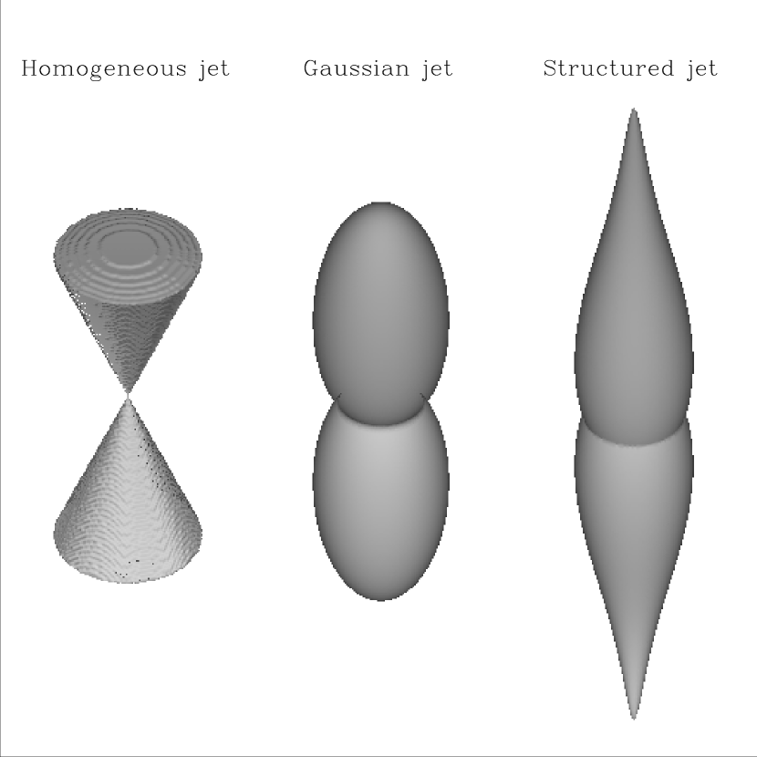
Figure 1: Cartoon of the three jet configurations discussed in this paper. The figure shows the energy per unit solid angle of the jets logaritmically scaled. The scale is different for each jet: it has been chosen in order to visually emphasize the characteristics of each configuration.

After the discovery of a significant, albeit small, degree of linear polarisation of the afterglow optical flux of GRB 990510 (Covino et al. 1999; Wijers et al. 1999), there have been several other detections of linear polarisation in a number of afterglows (see Covino et al. 2002 for review). Typically, the polarisation is observed to be at the 1-3 percent level (but see Bersier et al. 2003 for GRB 020405), with constant or smoothly variable level and position angle when associated with a relatively smooth lightcurve (e.g. GRB 020813, Gorosabel et al. 2004). When deviations from a smooth power-law decay in the lightcurve are instead present, polarisation curves show a certain degree of complexity (e.g. GRB 021004 Lazzati et al. 2003; Rol et al. 2003; GRB 030329 Greiner et al. 2003).

In order to observe polarisation, some kind of asymmetry is needed: this can be provided by patches of coherent magnetic field, as suggested by Gruzinov & Waxman (1999) and Gruzinov (1999). In addition, small regions in which the magnetic field has some degree of order could be amplified by scintillation (Medvedev & Loeb 1999), or by gravitational mini-lensing (Loeb & Perna 1998; Ioka & Nakamura 2001). In these cases the required degree of asymmetry is in the structure of the magnetic field, and not in the overall geometry of the fireball, which could even be spherically symmetric.

Recently Granot & Königl (2003) proposed that the required asymmetry might be provided by an ordered magnetic field embedded in the circum-burst material, possibly amplified when the shock propagates in it, to reach values close to equipartition with the energy density of the shocked material in the “pulsar wind bubble” scenario (Königl & Granot 2002).

A different class of models postulates that the fireball is jetted (i.e. the ejecta are collimated into a cone with half opening angle $\theta_{jet}$). In this case the observer likely sees the fireball off-axis, since the probability to be exactly on-axis is vanishingly small (Ghisellini & Lazzati 1999; Sari 1999, hereafter GL99 and S99, respectively). When the fireball bulk Lorentz factor $\Gamma$ is $\sim 1/(\theta_{jet}-\theta_{o})$ (where $\theta_{o}$ is the viewing angle) the emitting surface starts to be asymmetrical with respect to the line of sight. Moreover it is assumed that a magnetic field is compressed in the plane normal to the motion, analogous to what has been proposed for the jets of radio-loud active galactic nuclei (Laing 1980). Face-on observers would see a completely tangled magnetic field, but edge-on observers (in the comoving frame) would see an aligned field, and therefore would detect synchrotron polarised radiation. Since the fireball is moving with a high bulk Lorentz factor, the edge-on comoving observer corresponds to an observer in the lab located at an angle $\sim 1/\Gamma$. According to this idea, there is a tight link between the behaviour of the total and the polarised flux as a function of time. The light curve of the polarised flux has two maxima (corresponding to the presence of the two edges of the jet) with a position angle switched by $90^{\circ}$. The maxima occur just before and after the achromatic “jet” break in the light curve of the total flux. A main assumption of this model is that, at any given angle from the apex of the jet, the luminosity emitted per unit solid angle along the jet axis and along the jet borders is the same. Let us call jets with this energy structure “homogeneous” jets (HJs) (see Fig.1).

It is possible, instead, that the radiated power (per unit solid angle) along the jet axis is larger than what is emitted along the “wings”. If the wing energy distribution is a power-law, we refer to these configurations as “structured” jets (SJs) (see Fig.1). As Rossi, Lazzati & Rees (2002) (thereafter RLR02) and Zhang & Mészáros (2002) have demonstrated, if the luminosity per unit solid angle is $L(\theta)\propto\theta^{-a}$ with $a$ close to 2, then observers with a viewing angle $\theta_{\rm o}$ would see an achromatic jet break when $\Gamma\sim 1/\theta_{o}$. It is therefore possible that all GRB jets are intrinsically alike, having the same total intrinsic power and the same jet aperture angle: they appear different only because they are viewed along different orientations. If the jet were uniform, instead, they should have a large variety of aperture angles, to account for the different observed jet-break times (Frail et al. 2001).

As demonstrated analytically in RLR02 and more recently numerically by Salmonson (2003) (thereafter S03), it is difficult, on the basis of the observed light curve, to discriminate between homogeneous and structured jets (see also Granot & Kumar 2003). However, as described in this paper, the two models are markedly different in the polarisation properties of the produced afterglow flux. In both models the polarisation is produced because different parts of the emitting jet surfaces do not contribute equally to the observed flux. In the homogeneous jet model this starts to occur when $1/\Gamma$ becomes of the order of $\theta_{\rm jet}-\theta_{\rm{o}}$ (i.e. when the emitting surface available to the observer “touches” the near border of the jet). In the structured jet model, instead, the required asymmetry is built-in in the assumption that the emission is a function of $\theta$, so that the relevant emitting surface is never completely symmetric for off-axis observers.

Finally we consider a jet with a Gaussian luminosity distribution (Zhang & Meszaros 2002). This can be regarded as a more realistic version of the sharp edged standard jet: the emission drops exponentially outside the typical angular size ($\theta_{c}$), within which it is roughly constant (see Fig.1). Let us call it the “Gaussian jet” (GJ). It has been argued that this configuration can accomodate a unified picture of GRBs and X-ray flashes. The underlying assumptions is the presence of an emission mechanism for which the peak energy $E_{p}$ in the prompt emission is a decreasing function of the angular distance from the jet axis. In this way X-ray flashes would be the result of observing a GRBs jet at large angles. According to Zhang et al. (2003) the GJ would reproduce the observed correlation $E_{p}\propto E_{iso}^{1/2}$ (Amati et al., 2002), while under the same assumption the universal SJ and the “top hat” jet would face severe problems. We notice here, however, that the above correlation is still based on a very small database in the X-ray flashes regime (only two X-ray flashes are included) and should be confirmed by future observations. As regards afterglow properties, a GJ seen within the core produces lightcurves that are similar (but with smoother breaks) to the HJ’s ones (Granot & Kumar 2003). The luminosity variation with angle gives, as in the case of a SJ, a net polarisation without the need of edges and we show here that its temporal behaviour is indeed different from both the SJ’s and the HJ’s one.

The detailed analysis of the polarisation characteristics and their connection with lightcurves in the homogeneous jet, universal structured jet and in the Gaussian jet models is the main goal of this paper. In Section 2 we described the numerical code we have implemented to study these models. Some analytical and semi-analytical results have been derived by GL99 and S99, for a non-spreading jet and for a sideway expanding jet respectively. The simplified prescription assumed by S99 for the lateral expansion led to prediction of a third peak in the light curve of the polarised flux for an observer close to the border of the jet. In addition, GL99 did not consider, for simplicity, the effects of the different travel times of photons produced in different regions of the fireball, while S99 considered this effect by representing the viewable region as a thin ring centred around the line of sight: the ring has an angular size of $~{}\Gamma^{-1}$ and a constant width with respect to the ring radius. Our numerical approach allows us to include the effects of the different photon travel time and to analyze and compare different prescriptions for the side expansion of the fireball.

This paper is organised as follows. In §2 we present the model for the jet and for the magnetic field. In §3 we show the results for a homogeneous jet, in §4 those for a structured jet and in §5 those for a Gaussian jet. The comparison and discussion can be found in §6. Finally in §7 we derive and discuss our conclusions, adding possible complications to the models.

Throughout this paper the adopted cosmological parameters are $H_{0}=65$, $\Omega_{\lambda}=0.7$ and $\Omega_{m}=0.3$.

2 The Code

2.1 The Jet structure and dynamics

In this paper we show results obtained with two different codes. The first one is fully described in S03 while the second one is discussed in this section. The main difference between the two codes is in the treatment of the sideway expansion and dynamics in the non-relativistic phase. In the following we only remind the reader of the different assumptions adopted by S03 and refer the reader to the paper for more details.

We assume that the energy released from the engine is in the form of two opposite jets. They are described by the following distributions of initial Lorentz factor $\Gamma_{0}$ and energy per unit solid angle $\epsilon$ with respect to the jet axis ($\theta=0$):

$$\begin{array}[]{ll}\epsilon(\theta)=\frac{\epsilon_{c}}{\left(1+\left(\frac{\theta}{\theta_{c}}\right)^{(\alpha_{\epsilon}\,\beta_{\epsilon})}\right)^{\frac{1}{\beta_{\epsilon}}}}&\;\;\;\theta\leq\theta_{jet},\end{array}$$ (1)

$$\begin{array}[]{ll}\Gamma_{0}(\theta)=\frac{\Gamma_{c}}{\left(1+\left(\frac{\theta}{\theta_{c}}\right)^{(\alpha_{\Gamma}\,\beta_{\Gamma})}\right)^{\frac{1}{\beta_{\Gamma}}}}&\;\;\;\theta\leq\theta_{jet},\end{array}$$ (2)

where $\theta_{jet}$ is the jet opening angle, $\theta_{c}$ is the core angular size, $\epsilon_{c}=\epsilon(0)$ and $\Gamma_{c}=\Gamma(0)$. In the following, in order to make the comparison with the homogeneous jet easier, we will use preferentially the local isotropic equivalent energy, defined as $E_{iso}(\theta)=4\,\pi\,\epsilon(\theta)$. In Eqs. 1 and 2 $\alpha_{\epsilon},\alpha_{\Gamma}$ controls the shape of the energy and $\Gamma_{0}$ distributions in the wings, while $\beta_{\epsilon},\beta_{\Gamma}$ controls the smoothness of the joint between the jet core and its wings.

If $\alpha_{\epsilon},\alpha_{\Gamma}=0$, equations 1 and 2 describe the standard top hat model with sharp edges (homogeneous jet). If the observer line of sight is located within the jet, the observer detects the GRB prompt phase and its GRB afterglow (GA); if the viewing angle $\theta_{o}$ is larger then $\theta_{jet}$, he observes what it is called an orphan afterglow, an afterglow not preceded by the prompt $\gamma$-ray emission.

When $\alpha_{\epsilon}>0$, the code describes a structured jet; in this case $\theta_{jet}$ is assumed to be always much larger then the observer angle. In fact we consider here a boundless jet (the end of the wings are so dim that are undetectable), in contrast to the sharp edged homogeneous jet. If $\alpha_{\epsilon}=2$ and $\beta_{\epsilon}\to\infty$, the structured jet is that described in RLR02, while S03 adopts $\alpha_{\epsilon}=2$ and $\beta_{\epsilon}=1$.

For the Gaussian jet we use instead

$$\epsilon(\theta)=\epsilon_{0}\,\,e^{-\frac{\theta^{2}}{2\theta_{c}^{2}}}.$$ (3)

For simplicity we assume axial symmetry. Our initial Lorentz factor distribution satisfies $1/\Gamma\leq\theta$, therefore regions on the shock front with different $\Gamma_{0}$ and energy are causally disconnected and they evolve independently until $1/\Gamma=\theta$. In the numerical simulations we assume for all models a costant initial Lorentz factor across the jet, with $\Gamma_{0}=10^{4}$. With this choice the lightcurves shown in this paper (for observed times $\lower 2.15277pt\hbox{$\;\buildrel>\over{\sim}\;$}15$ min) are insensitive to the initial $\Gamma$ distribution. As a matter of fact, for any $\Gamma_{0}(\theta)\lower 2.15277pt\hbox{$\;\buildrel>\over{\sim}\;$}50$, the fireball deceleration starts earlier ($t_{d}\simeq 245s(E_{53}/n_{0}/\Gamma_{0,2}^{8})^{1/3}$) than the smallest time of the figures and afterwards the evolution follows the BM self similar solution and consequently the shown afterglow properties are independent from the initial Lorentz factor. If relativistic kinematic effects freeze out the lateral expansion or the pressure gradient prevents mixing, the different parts of the flow are virtually independent along their entire evolution. We allow each point of spherical coordinates ($r,\theta,\phi$) to evolve adiabatically and independently, as if it were part of a uniform jet with $\epsilon=\epsilon(\theta)$, $\Gamma_{0}=\Gamma_{0}(\theta)$ and semi-aperture angle $\theta$. Therefore, if the mixing of matter is unimportant this treatment is correct at any time, otherwise it gives an approximate solution for $1/\Gamma\gg\Delta\theta$. Actually numerical hydrodynamical simulations seem to suggest that $\epsilon(\theta)$ does not vary appreciably with time until the non-relativistic phase sets in (Kumar & Granot 2003) thus supporting our numerical approach.

The full set of equations that determine the dynamics of each patch of the jet is:

$$\Gamma=\frac{\sqrt{1+4\,\Gamma_{0}\,f+4\,f^{2}}-1}{2\,f},$$ (4)

(e.g. Panaitescu & Kumar 2000, thereafter PK00) where the parameter $f$ (the ratio of the swept-up mass to the initial fireball rest mass) is given by:

$$f=\frac{1}{M_{0}(\theta)}\int_{0}^{r}{r^{2}\Omega(r)\,\rho(r)\,dr},$$ (5)

where $M_{0}$ is the rest mass of the two (symmetric) jets, $\Omega(r)=4\pi\,(1-\cos\theta(r))$ is their solid angle and $\rho(r)$ is the ambient medium matter density. The evolution of the solid angle is described by:

$$\frac{d\theta}{dr}=\cos^{2}{\theta}\,\,\frac{c_{s}(\theta,r)}{c\beta\Gamma r}.$$ (6)

For the comoving lateral velocity $c_{s}$ we tested three different recipes. First, we analyze a non-sideways expanding (NSE) jet with

$$c_{s}=0.$$ (7)

then a sideways expanding (SE) one, either with a constant comoving sound speed (Rhoads 1999)

$$c_{s}\simeq c/\sqrt{3}$$ (8)

or with a more accurate treatment, which takes into account the behaviour of the sound speed as a function of the shock Lorentz factor:

$$c_{s}=c\,\sqrt{\frac{\hat{\gamma}(\hat{\gamma}-1)(\Gamma-1)}{1+\hat{\gamma}\,(\Gamma-1)}}$$ (9)

(Huang et al. 2000), where $\hat{\gamma}=\frac{4\,\Gamma+1}{3\Gamma}$.

In the code developed by S03 (see in particular S03 §2), it is assumed that both momentum and energy are conserved (Rhoads 1999):

$$\Gamma=\frac{\Gamma_{0}+f}{\sqrt{1+2\,\Gamma_{0}\,f+f^{2}}}.$$ (10)

This affects mainly the temporal slope of the lightcurve in the non-relativistic regime, since the jet does not follow the Sedov-Taylor solution. For the sideways expansion prescription S03 assumes that the lateral kinetic energy of the shock, in its radially comoving frame, is a constant proportion of the radial kinetic energy:

$$R_{k}=(\gamma^{\prime}_{\perp}-1)/(\gamma-1),$$ (11)

where $R_{k}$ (using S03’s notation) describes the shock efficiency to convert radial kinetic energy $(\gamma-1)$ in lateral kinetic energy ($\gamma^{\prime}_{\perp}-1$) and

$$\Gamma=\gamma\gamma^{\prime}_{\perp},$$ (12)

The jet dynamics in the trans- and non-relativistic phase is uncertain. If the two opposite jets do not merge ($\theta_{jet}$ is always $<90\degr$) when the dynamics becomes non-relativistic, the radial momentum should be conserved through all the evolution of the jet. This possibility depends strongly on the initial opening angle and on the assumed type of lateral expansion. For example, using the lateral velocity assumed by S03, initially narrow jets will not merge, because the sideways expansion, deriving its energy from the forward expansion, is soon exhausted. On the other hand, if, at late times, lateral spreading causes the jets to homogenize and become effectively spherically symmetric, then Eq. 4 is correct. For these reasons and the presence in literature of both treatments we compare and show in this paper results from both Eq. 4 and Eq. 10.

In Fig. 2 we show the opening angle of the jet vs. the shock radius for all sideways velocity prescriptions. The jet spreads more efficiently when the simpler prescription $c_{s}=c/\sqrt{3}$ is adopted while with Eq. 11 the expansion stalls out at fairly small angles ($\sim\theta_{j}(0)+\arctan{\sqrt{R_{k}}}$), since the jet is radially decelerating. Eq. 11 gives another interesting behaviour: the jet begins to laterally expand earlier than $\theta_{jet}(r)\sim 1/\Gamma$; this is because $R_{k}$ = 0.01,0.1 correspond to very large and supersonic initial lateral expansions. A direct comparison between the two sonic expansions (dotted and dashed lines) shows that a variable sound velocity (Eq. 9) gives a final $\theta_{jet}$ smaller than Eq. 8. Note however that this seems not to affect appreciably the resulting lightcurve (Fig. 4).

Figure 2: The opening angle of an homogeneous jet as a function of the distance from the explosion site for four different lateral velocities given by Eq. 7, Eq. 8, Eq. 9 and Eq. 11. The jet has an initial $\theta_{jet}$ of $10^{\circ}$, $\Gamma_{0}=10^{4}$, $E_{iso}=10^{53}$ and the external density is $n=10$ cm^-3. See text for discussion.

2.2 Spectrum and Luminosity

In order to isolate the effects of the jet structure on the emission and polarisation curves, we assume throughout this paper a constant density environment $\rho(r)=m_{p}\,n$ ($m_{p}$ being the proton mass and $n$ the number density). Polarisation curves derived here should be therefore compared only to data from afterglow with smooth lightcurves (Lazzati et al. 2003). Polarisation curves in a windy environment are similar to ISM ones, but characterised by a slower evolution (Lazzati et al. 2004).

The comoving intensity $I^{\prime}$ is assumed to be given by the synchrotron process only (Granot & Sari 2002); we do not include inverse Compton emission, because (for the adopted fiducial parameters) it can modify the observed afterglow lightcurve and polarisation curves only in the X-ray band after $\sim 10$ days (depending on the density, see e.g. Sari & Esin 2001). Therefore our results are accurate up to the X-ray band. We will comment on how the polarisation curves would be modified, should IC emission be included (§3.3.4).

In the shocked matter the injected electron Lorentz factor is

$$\gamma_{m}=\frac{m_{p}}{m_{e}}\,\epsilon_{e}\left(\Gamma-1\right),$$ (13)

where $m_{e}$ is the electron mass and $\epsilon_{e}$ is the fraction of kinetic energy given to electrons; the Lorentz factor of the electrons that cool radiatively on a timescale comparable to dynamical timescale (i.e. time since the explosion) is

$$\gamma_{c}=15\,\pi\,\frac{m_{e}\,c^{2}\,\sqrt{\Gamma^{2}-1}}{\sigma_{T}\,B^{2}\,r},$$ (14)

where $\sigma_{T}$ is the Thomson cross section and the comoving magnetic field $B$ is given by:

$$B=\sqrt{32\,\pi\,\epsilon_{B}\,m_{p}\,c^{2}\,n}\,\sqrt{\Gamma^{2}-1}.$$ (15)

where $\epsilon_{B}$ is the fraction of internal energy that goes to the magnetic field. Note that Eq. 14 and Eq. 15 are different from those given by PK00 that are not accurate in the trans and sub-relativistic regimes. The corresponding synchrotron frequencies are:

$$\nu_{i}=0.25\,\frac{e\,\gamma_{i}^{2}\,B}{m_{e}\,c},$$ (16)

where the constant (0.25) is calculated for an electron energy distribution index $p=2.5$ (PK00), $e$ is the electron charge, $i=m$ for the peak frequency and $i=c$ for the cooling frequency. The synchrotron self absorption frequency is given by:

$$\nu_{a}=\nu_{i}\,\tau_{i}^{3/5},$$ (17)

where $i=m$ in the slow cooling regime and $i=c$ in the fast cooling regime; $\tau_{i}=\frac{5\,e}{3}\,\frac{n\,r}{B\gamma_{i}^{5}}$ is the optical thickness at $\nu_{i}$. The comoving peak intensity $I^{\prime}_{p}$ is

$$I^{\prime}_{p}=\frac{P^{\prime}\,n\,r\,}{\nu_{m}},$$ (18)

where $P^{\prime}=\frac{4}{3}\,\sigma_{T}\,c\,\frac{B^{2}}{8\,\pi}\left(\gamma_{m}^{2}-1\right)$ is the total power emitted by relativistic electrons with Lorentz factor $\gamma_{m}$ and isotropic distribution of pitch angles. The local observed luminosity is then computed through:

$$dL(t,\theta,\phi)=I^{\prime}\,\delta^{3}\,r^{2}\,\sin{\theta}\,d\theta\,d\phi$$ (19)

where $\delta=\frac{1}{\Gamma\,(1-\beta\cos{\tilde{\theta}})}$ is the relativistic Doppler factor and $\tilde{\theta}$ is the angular distance from the line of sight. The observed arrival time $t$ of photons can be computed as follows:

$$t=t_{lab}-\frac{r}{c\cos\tilde{\theta}},$$ (20)

where the time in the laboratory frame $t_{lab}$ at which the photons were emitted is

$$t_{lab}=\int\frac{dr}{\beta_{sh}c},$$ (21)

where $\beta_{sh}\,c$ is the shock front speed. The Lorentz factor $\Gamma_{sh}$ of this front is related to the Lorentz factor $\Gamma$ of the shocked matter behind it (Eq. 4) by $\Gamma_{sh}=1+\sqrt{2}\,\left(\Gamma-1\right)$ (e.g. Sari 1997).

2.3 The emitting volume

For a given time, Eq. 20 describes the locus of points from which photons arrive simultaneously at the detector (equal arrival time surfaces EATS). The EATS for a structured jet are shown in Fig. 3, where the observer is located to the right. Unlike the homogeneous case (e.g. Panaitescu & Mészáros 1998; Granot, Piran & Sari 1999), the EATS shape in the SJ depends on the viewing angle. This is because, for relativistic effects, each line of sight mimics a homogeneous jet with different parameters: $\theta_{jet}\simeq 2\,\theta_{o}$, $E_{iso}\simeq E_{iso}(\theta_{o})$ and $\Gamma_{0}\simeq\Gamma_{0}(\theta_{o})$ (RLR02).

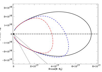
Figure 3: The Equal Arrival Time Surfaces for a a SJ seen at $0^{\circ}$ (solid line), $6^{\circ}$ (dashed line) and $12^{\circ}$ (dot-dashed line) from the jet axis. The straight dotted lines mark the position of the jet axis and the horizontal dashed line is the line of sight. For $\theta_{o}=0$ of course the dotted line overlaps the dashed line. The jet parameters are: external density $n=1$ cm^-3, core dimension $\theta_{c}/\theta_{jet}=0.1$, $E_{c}=10^{54}$ erg, $\Gamma_{c}=10^{4}$, $\alpha_{\epsilon}=2$ and $\alpha_{\Gamma}=2$. EATSs clearly depend on the observer position: each line of sight mimics an homogeneous jet with different energy, Lorentz factor and $\theta_{jet}$.

The emission that the observer detects at time $t$ does not come only from a thin layer near the EATS; in fact it comes from a sizable fraction of the volume behind it whose width is $\sim\frac{r}{2\,\Gamma_{sh}}$. Therefore, for each $t$, $\theta$ and $\phi$, we integrate equation 19 also over this emitting volume, using the Blandford & Mckee (1976, hereafter BM) solution for the Lorentz factor of the shocked gas behind the shock front (Granot, Piran & Sari 1999). This calculation for the observed flux is strictly valid for $\nu>\nu_{a}$, since we do not take into account self absorbing effects.

2.4 Magnetic field configuration and linear polarisation

The magnetic field configuration we adopt is obtained by compressing, in one direction, a volume containing a random magnetic field: it has some degree of alignment seen edge-on while it is still completely tangled on small scales in the uncompressed plane. This could be the geometry of a magnetic field produced by the blastwave that, sweeping up the external medium, could confine the field in the sky plane. It may also be the natural configuration of shock generated magnetic fields (Medvedev & Loeb 1999).

Since the fireball is relativistic, the circle centered around the line of sight, with angular aperture $\tilde{\theta}\simeq 1/\Gamma$, is the region contributing the most to the observed emission and the photons that reach the observer from the borders of that circle are emitted at $\theta^{\prime}=90^{\circ}$ in the comoving frame. Therefore the light coming from an angle $\tilde{\theta}\simeq 1/\Gamma$ has the maximum degree of polarisation $P_{0}$ while the light travelling along the line of sight is unpolarised (see Fig. 1 in GL99). We assume $P_{0}=60\%$. In the comoving frame this value decreases with the angular distance ($\theta^{\prime}$) to the line of sight as

$$P(\theta)=P_{o}\frac{\sin^{2}(\theta^{\prime})}{1+\cos^{2}(\theta^{\prime})},$$ (22)

(Laing 1980). The Lorentz transformations of angles give us the relation between $\tilde{\theta}$ and $\theta^{\prime}$:

$$\cos{\theta^{\prime}}=\frac{\cos{\tilde{\theta}}-\beta}{1-\beta\,\cos{\tilde{\theta}}}$$ (23)

$$\sin{\theta^{\prime}}=\Gamma\sin{\tilde{\theta}}\,\,\left(1+\beta\,\cos{\theta^{\prime}}\right).$$ (24)

In terms of the Stokes parameters, $Q$, $U$, $V$, and local luminosity $dL$ (equivalent to the Stokes parameter $I$) $P(\theta)$ can be described as a vector with components:

$$dQ(t,\theta,\phi)=P(\theta)dL(t,\theta,\phi)\cos(2\phi),$$ (25)

$$dU(t,\theta,\phi)=P(\theta)dL(t,\theta,\phi)\sin(2\phi).$$ (26)

and

$$V=0$$ (27)

Integrating Eq. 26 and Eq. 25 over the EATS we obtain the intensity of the observed total polarisation vector at a time $t$:

$$\mathcal{P}(t)=\frac{\sqrt{Q(t)^{2}+U(t)^{2}}}{L(t)},$$ (28)

which is actually the fraction of flux linearly polarised. The direction of the total polarisation vector is then

$$\phi(t)=0.5\,\arctan{\frac{U(t)}{Q(t)}}.$$ (29)

Figure 4: Comparing the $R$ band ($7\times 10^{14}Hz$) lightcurves resulting from different sideways expansions shown in Fig. 2, where the jet parameters are given. The shock parameters are: $p=2.5$, $\epsilon_{e}=0.01$ and $\epsilon_{B}=0.005$. An on-axis observer ($\theta_{o}=0$) has been assumed here. SE jets with constant (dashed line) and variable (dotted-line) sonic lateral velocity give very similar lightcurves. SE jets with supersonic lateral velocities (“dash-dot” and “dash-3 dots” lines) have been divided by a factor of $10$ for clarity. They have more extreme spreading jet features (smoothness of the break, late time break) and due to a different dynamics they do not follow the Sedov-Taylor solution in the non-relativistic regime.

Figure 5: The same as Fig. 4 for the polarisation curves. SE jets with constant (dashed line) and variable (dotted-line) lateral velocity give almost indistinguishable polarisation curves (the second highest curve). Most of the time SE jets have a lower degree of polarisation than the NSE jet (solid line). Note that the larger the lateral velocity, the lower the polarisation.

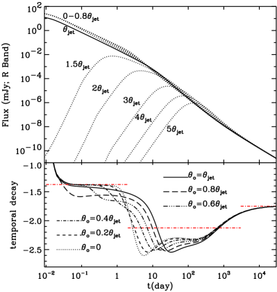
Figure 6: Lightcurves (upper panel) and power-law indices as a function of time (lower panel) for a NSE homogeneous jet ($\alpha_{\epsilon}=\alpha_{\Gamma}$=0 and $\beta_{\epsilon}=\beta_{\Gamma}=1$), seen from different viewing angles. The parameters are $\Gamma_{0}=10^{4}$, $E_{iso}=10^{53}$ erg, $\theta_{jet}=10^{\circ}$, $n=10\,$cm^-3, $\epsilon_{e}=0.01$, $\epsilon_{B}=0.005$, $p=2.5$, $\nu=7\times 10^{14}$ Hz and $z=1$. For these parameters the $R$ band is beyond the cooling frequency. The curves corresponding to $\theta_{o}=0\to\theta_{o}=0.8\theta_{jet}$ are shown but not labelled one by one for clarity. The black solid line corresponds to $\theta_{o}=\theta_{jet}$, that shows a sort of intermediate behavior between GRB afterglows ($\theta_{o}<\theta_{jet}$) and orphan afterglows ($\theta_{o}>\theta_{jet}$). The temporal decay for $GRB$ afterglows is shown in the lower panel. The horizontal dash-dotted lines are the standard analytically predicted slopes for the pre-break power-law $\alpha_{1}=-\frac{(3p-2)}{4}=-1.375$, the post-break power-law $\alpha_{2}=\alpha_{1}-\frac{3}{4}=2.125$ and the non-relativistic phase $\alpha_{3}=-\frac{(3p-4)}{2}=1.75$. The post break slope is steeper than predicted by a factor $\sim 1/4$. Moreover as $\theta_{o}$ increases, the break becomes smoother (see also Tab. 1), and the time of the turnover increases. See text for discussion.

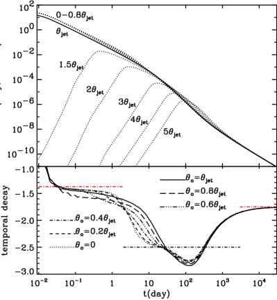
Figure 7: Same as Fig. 6, but for a SE jet, with a comoving velocity given by Eq. 9. The jet and shock parameters are the same as Fig. 6. Here the post break slope given by the standard calculation is $\alpha_{2}=-p=2.5$, but again we find $\alpha_{2}$ steeper by a factor of $\sim 1/4$, immediately after the break. The lower panel shows that the time break increases with $\theta_{o}$, as well as the smoothness of the break, though only mildly (see also Tab. 1). See text for discussion.

3 Homogeneous jet: results

In Fig. 4 and Fig. 5 we compare the light and polarisation curves resulting from different recipes for the lateral expansion (§2.1). The expansions given by Eq. 8 and Eq. 9 produce very similar temporal behaviors; therefore in the following we show results which are strictly valid for a variable sound speed but the same discussion holds for $c_{s}=c/\sqrt{3}$. The lightcurves shown in Fig. 4 are all consistent with the same pre and post-break temporal slopes for a relativistic jet. However the curves corresponding to a jet that obeys the conservation of momentum (Eq. 10, the dash-dotted and dash-3 dotted lines) does not follow a Sedov-Taylor model ($\beta\propto r^{-3/5}$ and flux $F(t)\propto t^{-\frac{(3p-4)}{2}}$, for $\nu>\nu_{c}$) in the non-relativistic regime but $\beta\propto r^{-3}$ and $F(t)\propto t^{-43/16}$. Then in this latter case the flux falls off more rapidly while in the former case the lightcurve tends to flatten. We anticipate that in both cases the non-relativistic slopes do not depend on the viewing angle but only on the spectrum, contrary to the temporal slopes in the relativistic regime (see also Fig. 6, 7).

Fig. 4 and Fig. 5 also show that a SE jet has

• a smoother break in the lightcurve,

• a later time break,

• smaller polarisation peaks,

compared to a NSE jet and these characteristics are even more evident for jets with a supersonic sideways expansion.

All these features (among others) are discussed in more details in the following, comparing a NSE jet with a jet undergoing a sideways expansion given by Eq. 9. For a jet evolution following Eq. 11 we refer the reader to S03, where a more complete discussion is given.

3.1 Lightcurve: the shape of the break

The R band lightcurve for a NSE and for a SE homogeneous jet are shown in Fig. 6 and Fig. 7 respectively. They show interesting features, some of which have never been discussed before. In the lower panels the temporal index $\alpha$ (defined as $F(t)\propto t^{\alpha}$) is plotted versus time. We call $\alpha_{1}$,$\alpha_{2}$ and $\alpha_{3}$ the pre-break, the post-break and the non-relativistic slope respectively. The horizontal dot-dashed lines show the expected slopes from on-axis standard calculations.

3.1.1 $\alpha_{2}$

The “standard” post-break slopes (central dot-dashed lines in Fig. 6 and Fig. 7, lower panels) are calculated considering the loss of the emitting area from a spherical blast wave $(1-\cos\Gamma^{-1})$ to a conical one $(1-\cos\theta_{jet})$. For the SE jet we also consider the more rapid deceleration due to the increase of the shock front surface (Rhoads 1999; Sari, Piran & Halpern 1999). In both cases the surface brightness is supposed to be the same across the surface of the jet at all times. For $\nu>\nu_{c}$ the expected breaks are $\Delta\alpha_{nse}=\frac{3}{4}$ for a NSE jet and $\Delta\alpha_{se}=\frac{(p+2)}{4}=1.125$ for a SE one.

In fact we find that the flux after the break falls off more rapidly than expected, and this effect is more evident as the electron energy distribution $N(\gamma)\propto\gamma^{-p}$ becomes steeper. This can be understood by taking into account the effect of EATS. When $r/\Gamma<r\,\theta_{jet}$ the visible area can be schematized as a bright ring with radius $r/\Gamma$ and width $\Delta$ ($20\%-40\%$ of the whole area) that surrounds a dimmer uniformly emitting surface (e.g. Granot et al. 1999). When $r/\Gamma>r\,\theta_{jet}+\Delta$ only the dimmer emitting surface is visible. As a consequence after the break the deficit in the observed flux is bigger and $\alpha_{2}$ is steeper than considering, at any time, a uniform emitting surface. The effect is more pronounced for higher values of $p$ since the surface brightness contrast between the centre and the ring increases. When $r/\Gamma\gg r\,\theta_{jet}+\Delta$ the lightcurve decay index should tend to the standard slope, because the jet surface emits almost homogeneously; in fact only in the case of a very narrow jet ($\theta_{jet}<1^{\circ}$) this asymptotic slope is reached: wider jets lightcurves break later and they enter the trans-relativistic phase soon after the break, tending towards $\alpha_{3}$.

3.1.2 $\alpha_{1}$

Similarly the pre-break slope presents deviations from the standard calculations for a spherical symmetrical blastwave ($\alpha_{1}=\frac{-(3p-2)}{4}$: Fig. 6 and Fig. 7, lower panels, horizontal line on the left). If the jet is very narrow (less than few degrees) the lightcurve will not exhibit (depending on $\Gamma_{0}$) this first branch. For wider jets (as in our examples) the value $\frac{-(3p-2)}{4}$ is strictly followed only in the case of a NSE jet for observers around the line of sight.

3.1.3 $\alpha_{3}$

On the other hand the non-relativistic regime offers a lightcurve branch slope independent of the spreading and the viewing angle. This holds for any frequency band. However, uncertainties in the dynamics during the trans-relativistic phase (see §2.1) hamper the possibility to derive the electron distribution power-law index even at late stages.

3.2 Lightcurve: the time of the break

The lower panels of Fig. 6 and Fig. 7 show, in addition, how the jet-break and the temporal behaviour around it change with the off-axis angle. As the viewing angle increases the transition between $\alpha_{1}$ and $\alpha_{2}$ is smoother (GL99) and the break time (when $\alpha\simeq\frac{(\alpha_{1}+\alpha_{2})}{2}$) is retarded.

To obtain more quantitative results we fit the lightcurves $F(t)$ with a smoothly joined broken power law (SBP),

$$F(t)=\frac{2\,F_{b}}{\left[\left(\frac{t}{t_{b}}\right)^{\alpha_{1}\,s}+\left(\frac{t}{t_{b}}\right)^{\alpha_{2}\,s}\right]^{1/s}},$$ (30)

(Beuermann et al. 1999), where $s$ is the smoothness parameters and $F_{b}$ the normalisation ($F_{b}=F(t_{b})$ for $s=1$). The smoothness parameters is a measure of the shape of the lightcurve around the break: the lower its value the smoother the two asymptotic slopes are joined together over the break. The fit is performed over the range $0.01\,t_{b}\leq{}t\leq 100\,t_{b}$ and assigning an uncertainty of $10\%$ to each point.

The results are summarised in Tab. 1 where $t_{b}$ and $s$ are given as a function of $\theta_{o}/\theta_{jet}$. For NSE jet lightcurves, the fit gives break times that range from $1.86$ days for a on-axis observer to $5.7$ days for $\theta_{o}/\theta_{jet}=0.8$, while for a SE jet $t_{b}=3.57$ days for $\theta_{o}=0$ and $t_{b}=7.44$ days for $\theta_{o}/\theta_{jet}=0.8$. However changing the time interval of the fitting can result in a variation of the estimated $t_{b}$ of a factor of 2, while the positive correlation between $t_{b}$ and $\theta_{o}$ generally holds. Tab. 1 shows also that $s$ decreases for larger $\theta_{o}$ and the effect is greater when lateral expansion is not dynamically important (see also Fig. 4 in GL99). The bottom line of this discussion is that the break time is an ill-defined quantity, since the function generally used for data fits is only a rough approximation to the real shape of the afterglow lightcurve. Systematic uncertainties on the measure should be considered, especially when the break time is used to infer the opening angle of the jet to derive the beam-corrected energy output of GRBs (e.g. Berger et al. 2003).

Figure 8: Polarisation curves for a homogeneous NSE jet, corresponding to the lightcurves shown in Fig. 6. The $x$ axis is the time since the trigger divided by the on-axis lightcurve time break $t_{b}=1.86$ days. These curves may have to be rescaled by a factor $<1$, since $P_{0}=60\%$ is taken arbitrary. For $P<0$ the vector is in the plane containing the line of sight and the jet axis, while for $P>0$ is rotated of $90^{\circ}$. The black solid lines correspond to $\theta_{o}=\theta_{jet}$ and $\theta_{o}=0.2\theta_{jet}$. GRB afterglows always show two peaks, with the second one higher than the first, and with polarisation angles rotated by $90^{\circ}$. Orphan afterglows’ polarisation curves have two peaks, with the same angle, for $\theta_{o}<3\theta_{jet}$ that eventually merge into a single maximum for larger viewing angles; the polarisation at the peak grows with $\theta_{o}$. The peak polarisation for an orphan afterglow can therefore be a factor $\sim 2.5$ larger than what it is expected at $\theta_{o}=\theta_{jet}$.

Figure 9: Same as Fig. 8 but for a homogeneous SE jet. The corresponding lightcurves are shown in Fig. 7. The $x$ axis is the time since the trigger divided by the on-axis lightcurve time break $t_{b}=3.57$ days. All the main features are the same as for the $NSE$ jet but the expected polarisation values are lower and the two maxima in the orphan afterglows curve merge for $\theta\simeq 6\theta_{jet}$, where the maximum value of polarisation is reached. Then the polarisation at the peak decreases. The polarisation for an orphan afterglow can therefore be a factor $\sim 2.6$ larger than what it is expected at $\theta_{o}=\theta_{jet}$.

3.3 Polarisation curves

The polarisation curves we obtain are given in Fig. 8 and Fig. 9.

3.3.1 GRB afterglows

Homogeneous GRB afterglow polarisation curves ($\theta_{o}/\theta_{jet}\leq 1$) always show two peaks, with the second higher then the first one, with pitch angles rotated by $90^{\circ}$. For $\theta_{o}/\theta_{jet}\lower 2.15277pt\hbox{$\;\buildrel>\over{\sim}\;$}0.6$ this change in the direction of the polarisation vector ($P=0$) happens before the break-time measured by an on-axis observer, while for smaller angles it happens slightly after.

3.3.2 Orphan afterglows

The polarisation curve of orphan afterglows ($\theta_{o}/\theta_{jet}\geq 1$) has two peaks, with the same position angle, that eventually merge in a single maximum. For a NSE jet the polarisation at the peak grows with $\theta_{o}$, tending towards $P_{0}$ (Fig. 8), while with sideways expansion the peak value reaches a maximum around $\theta_{o}\sim 7\theta_{jet}$ and then it slowly decreases; in both cases the polarisation peak for an orphan afterglow can be a factor $\sim 2.5-2.6$ larger than what it is expected at $\theta_{o}=\theta_{jet}$.

3.3.3 Comparison with previous results

The polarisation curves for a NSE jet with $\theta_{o}<\theta_{jet}$ have been previously published by GL99, which did not consider EATS. Their curves have our very same temporal behaviour, but their polarisation peaks are lower than ours by a factor from 2 to 4, depending on the viewing angle. This is the result of adding EATS to the computation. In this case the received intensity, at any given time, peaks at an angular distance $1/\Gamma$ from the line of sight, just where the linear polarisation is maximised (see Eq. 22, Eq. 26 and Eq. 25). As a result, the total expected polarisation is higher than for a homogeneously emitting surface. S99 and Granot & Königl (2003) have instead explored the polarisation for a spreading jet. The first author uses a simplified model in which the opening angle does not change until $\frac{1}{\Gamma}<\theta_{jet}$ and then $\theta_{jet}$ increases as $1/\Gamma$; as a consequence he expects a third polarisation peak to appear at later times for large off-axis angles, while for small viewing angles only one peak should be visible. With our complete calculation of the evolution of the opening angle of the jet we do not obtain either of these effects (see Fig. 9). The reason is that the visible area ($1/\Gamma$) crosses both the nearest and the farthest edge of the jet for any off-axis angle and then $1/\Gamma$ remains always greater than $\theta_{jet}$. Therefore for a HJ, afterglow polarisation curves always have only two peaks with orthogonal polarisation angles, for all the sideways expansion models considered in this paper. Granot et al. (2002) have extended the computation also to orphan afterglows. They obtain

• higher value of polarisation for $GRB$ afterglows compared to ours with the first peak always greater then the second one (unlike what our curves show);

• for $\theta_{o}/\theta_{jet}=0.25$ only one peak is visible;

• an orphan afterglow peak can have a polarisation degree which is larger than what observed by an on-axis observer, but only by a factor 2.

These effects are due to an error in their program, pointed out recently by the authors themselves (see Granot & Königl 2003). The results of their corrected code are in general agreement with ours (Granot private communication).

NSE SE $\theta_{o}/\theta_{jet}$ $\frac{t_{b}}{t_{b}(0)}$ $s$ $\frac{t_{b}}{t_{b}(0)}$ $s$ 0 1 8.36 1 1.07 0.2 1.01 4.34 1.06 0.96 0.4 1.12 1.79 1.25 0.76 0.6 1.67 0.86 1.73 0.55 0.8 3.07 0.60 2.09 0.55

Table 1: This table summarises some results from the modelling with a SBP (Eq. 30) of the lightcurves shown in Fig. 6 ($NSE$ jet) and Fig. 7 ($SE$ jet). The break time $t_{b}$ is given as a multiple of the $t_{b}$ fitted by an on-axis observer [$t_{b}(0)$]. Note that the time at which the curve changes slope is postponed as the angular distance from the jet axis increases. The smoothness parameter $s$ of the break in a lightcurve is a measure of the break shape: the higher its value, the sharper is the transition between the two asymptotic slopes. The table shows that $s$ decreases with the off-axis angle. This effect is more evident for a $NSE$ jet.

Figure 10: Lightcurves (upper panel) and polarisation curves (lower panel) for a NSE jet seen at $\theta_{o}=0.6\theta_{jet}$ in three different spectral ranges: $F(\nu)\propto\nu^{1/3}$ (dot-dashed line, usually in the radio) $F(\nu)\propto\nu^{-(p-1)/2}$ (usually in the optical, solid line) and $F(\nu)\propto\nu^{-p/2}$ (usually in the X-rays, dashed line).The jet and shock parameters are the same as Fig. 6. $t_{b}=3.66$ days. The X-ray lightcurves has been rescaled by a factor $10^{3}$ for clarity.

3.3.4 Multiwaveband polarisation

Polarisation due to synchrotron emission is in principle present at any wavelength. In Fig. 10 we show the light and polarisation curves for the same GRB afterglow observed at a frequency $\nu_{o}$ in three different spectral branches: $\nu_{a}<\nu_{o}<\nu_{m}$, $\nu_{m}<\nu_{o}<\nu_{c}$ and $\nu_{c}<\nu_{o}$, for an observer at $\frac{\theta_{o}}{\theta_{jet}}=0.6$. In the following we refer to them as the “radio” branch, the “optical” branch and the $X$-ray branch respectively, since each waveband usually stays on that particular branch for most of the afterglow evolution (depending on fireball and shock parameters).

Fig. 10 shows that while the polarisation curves in the $R$ and X-ray bands are very similar, the radio curve has a significantly lower degree of polarisation. Disticnt from the other lightcurves, the radio flux increases with time before the break ($F_{\nu}\propto t^{1/2}$). It should fall asymptotically as $F_{\nu}\propto t^{-1/3}$ afterwards but the trans-relativistic phase sets in and eventually the flux rises again ($F_{\nu}\propto t^{8/5}$) following the non-relativistic temporal slope (Frail, Waxman & Kulkarni 2000).

We note that generally a spectral transition occurs in the radio band (8.5 GHz) at late times, when the peak frequency becomes smaller than the observed radio band ($\nu_{a}<\nu_{m}<\nu_{o}$). This causes a third peak to appear in the radio polarisation curve, since in the radio curve joins the optical one; on the other hand the radio lightcurve undertakes a spectral break and eventually follows the optical lightcurve temporal decay ($F_{\nu}\propto t^{-3(p-1)/4}$ before the jet break and $F_{\nu}\propto t^{-3p/4}$ after). In our calculations for the radio polarisation we do not take into account the effects of Faraday rotation: as long as $\Gamma>2$ this effect should be negligible, since the electrons are all highly relativistic, with $\gamma_{m}>100$. In the trans-relativistic phase its effect can be sizable and it could even wash out the intrinsic small degree of radio polarisation.

The $X$-ray polarisation curve can be affected by the contribution of the inverse Compton flux; in particular after $10-15$ days it may depolarise the synchrotron flux, depending on the external density. However faint fluxes are usually observed at this epoch, too faint for detection by any X-ray polarimeter conceivable in the near future. In fact, detection of polarisation in the $X$-ray band will probably be possible only within few hours from the trigger, when the synchrotron flux positively dominates the inverse Compton emission.

3.4 Summary

In this section we have described separately lightcurves and polarisation curves for homogeneous jets. The variation of viewing angle however affects both quantities. As the off-axis angle increases the break time increases and since the minimum in the polarisation curves occurs around $t_{b}(\theta_{o})$, it is delayed as well. Moreover the degree of polarisation increases at the peaks while the break shape becomes smoother. These joint characteristics should, in principle, be observable and be helpful for testing the model.

4 Structured jet: results

As a general result, our more sophisticated simulations confirm all the features we described in RLR02 for the lightcurve of a SJ: it is very similar to the lightcurve of an HJ seen on-axis with same energy per solid angle and $\theta_{jet}=2\theta_{o}$. On the other hand, we show that the polarisation curves for a SJ present key-features that allow us to spot the underlying jet structure.

4.1 Lightcurves

The temporal index $\alpha$ of a SJ lightcurve is shown in the lower panels of Fig. 11 and Fig. 12 for $\alpha_{\epsilon}$=2, $\beta_{\epsilon}$=1 and $\beta_{\Gamma}$=0. Similar to the HJ, a SJ’s lightcurve for $\theta_{o}>$ few degrees can be approximated as a broken power-law; moreover the same asymptotic slopes ($\alpha_{1}$, $\alpha_{2}$, $\alpha_{3}$) for an homogeneous jet (see §3.1) describe as well the temporal behaviour of a SJ’s lightcurve.

It can be noticed that for viewing angles within the core ($\theta_{o}\leq\theta_{c}$) the observed lightcurves are similar to those expected from very narrow HJs: the break happens so soon that the first power-law branch is missing while after the break there is enough time to reach $\alpha_{2}$ and follow that slope until the non-relativistic transition sets in. For larger viewing angles the situation is quite the reverse: as the $\theta_{o}$ increases the lightcurves have time to follow more strictly the standard value for $\alpha_{1}$ but there is less and less time to reach $\alpha_{2}$ before entering the sub-relativistic phase. This is the same behaviour observed in HJs lightcurve as the jet opening angle increases. Another point of similarity with HJ’s lightcurves is that (as discussed in §3.1.1 for HJs) the flux falls off more rapidly after the break than expected by standard calculations: this effects increases with the off-axis angle. Distinct from the HJ, the SJ lightcurves also present a flattening before the break that increases with the off-axis viewing angle. The deviations from the standard slopes before and after the break are of the same order.

We can conclude that HJ’s and SJ’s lightcurves can be described only roughly by broken power-laws and certainly only for a specific range of viewing angles.

4.1.1 The shape of the break

To quantify the sharpness of the break we again fit the simulated lightcurves with Eq. 30 and the results are summarised in Table  2. The smoothness parameter $s$ increases and then saturates around $\theta_{o}/\theta_{c}=8$, where the fit yields an extremely sharp break (the best fit is actually with a simple broken power-law rather than a SBP). A $NSE$ jet has sharper jet breaks compared to a $SE$ jet, but the relation between $s$ and the off-axis angle is similar. This relation is actually different from that discussed for the HJ (§3.2), where the break becomes smoother and smoother as $\theta_{o}$ increases.

4.1.2 The time of the break

The similarity between HJ and SJ lightcurves becomes more quantitative if we measure the break-time as a function of the viewing angle. The break time $t_{b}$ increases with the viewing angle and the general trend can be fitted by a power law:

$$t_{b}\propto(\theta_{o}/\theta_{c})^{2}$$

(see Tab.2). We underline that $t_{b}\propto\theta_{o}^{2}$ is predicted by the structured model with $\alpha_{\epsilon}$=2 and by the HJ model with constant total energy (once $\theta_{o}$ is replaced by $\theta_{jet}$).

One difference between the HJ and the SJ is that, for the same set of parameters, the SJ break time equals that of the HJ if $\theta_{jet}\sim 2\,\theta_{o}$ (RLR02) (see also Fig. 18). This factor comes from the two different origins of the break in the lightcurve: the HJ simply breaks when the edge of the jet comes into view ($\Gamma\simeq\theta_{jet}^{-1}$), while the structured jet breaks when $\Gamma_{c}\simeq\theta_{o}^{-1}$. The following simplified calculation aims to show that a HJ (with the same parameters as a SJ and $E_{iso}=E_{iso}(\theta_{o})$) tends to have an earlier break time if $\theta_{jet}=\theta_{o}$ and thus a larger opening angle (of the order of $\sim 2\theta_{o}$) is needed to have a reasonable agreement between the two break times. The break times ratio for a non spreading jet is

$$\frac{t_{jet,s}}{t_{jet,h}}=\biggl{(}\frac{\theta_{o}}{\theta_{jet}}\biggr{)}^{8/3}\left(\frac{\theta_{o}}{\theta_{c}}\right)^{2/3},$$ (31)

where $t_{jet,s}=\frac{R_{jet,c}}{c}\,(1-\beta\cos(\theta_{o}))$ is the observed break time for SJ ($R_{jet,c}$ being the radius at which $\Gamma_{c}=1/\theta_{o}$) and $t_{jet,h}=\frac{R_{jet}}{2\,c}\theta_{jet}^{2}$ is the break time for an HJ seen on-axis ($R_{jet}$ being the radius at which $\Gamma\sim 1/\theta_{jet}$). In Eq. 31 and below in Eq. 32 we assume the same isotropic equivalent energy along the line-of-sight and that $\Gamma_{0}$ does not depend on $\theta$; for a spreading jet we get instead

$$\frac{t_{jet,s}}{t_{jet,h}}=\biggl{(}\frac{\theta_{o}}{\theta_{jet}}\biggr{)}^{8/3}\left(1+\ln{\frac{\theta_{o}}{\theta_{c}}}\right),$$ (32)

where the logarithmic term takes into account the exponential behaviour of $\Gamma_{c}$ for $\Gamma_{c}<\theta_{c}^{-1}$. If we impose then that the structured and homogeneous jets lightcurves break at the same time Eq. 31 gives $1.3\lower 2.15277pt\hbox{$\;\buildrel<\over{\sim}\;$}\frac{\theta_{jet}}{\theta_{o}}\lower 2.15277pt\hbox{$\;\buildrel<\over{\sim}\;$}2.5$ and Eq. 32 give s $1.3\lower 2.15277pt\hbox{$\;\buildrel<\over{\sim}\;$}\frac{\theta_{jet}}{\theta_{o}}\lower 2.15277pt\hbox{$\;\buildrel<\over{\sim}\;$}1.8$ for $2\lower 2.15277pt\hbox{$\;\buildrel<\over{\sim}\;$}\frac{\theta_{o}}{\theta_{c}}\lower 2.15277pt\hbox{$\;\buildrel<\over{\sim}\;$}40$.

4.2 Polarisation curves

The polarisation curves of a structured jet with $\alpha_{\epsilon}$=2 and $\beta_{\Gamma}=$0 present all the same main features, regardless the adopted comoving lateral speed. As examples, we show a $NSE$ jet (Fig. 13) and a jet expanding with a supersonic lateral velocity (Eq. 11; Fig. 14). The $SE$ jets exhibit a lower degree of polarisation and wider peaks than $NSE$ jets; in particular for a supersonic lateral velocity, the lateral expansion starts earlier than $\theta_{jet}(r)\sim 1/\Gamma$ (see Fig. 2) and a higher degree of polarisation is present at very early times. Three major features characterize all the polarisation curves resulting from such SJs:

• There is only one maximum in the polarisation curve. Since the jet is intrinsically inhomogeneous the degree of polarisation is greater than zero, albeit small, even at early times. As the visible area ($\sim 1/\Gamma$) increases, the brighter inner part weights more in the computation of the total polarisation (Eqs. 25, 26 and  28) that increases until $1/\Gamma\sim\theta_{o}$. This is the configuration with the largest degree of asymmetry within the visible area and therefore it coincides with a maximum in the polarisation curve. As $1/\Gamma$ becomes larger than $\theta_{o}$ the degree of asymmetry decreases along with the polarised flux.

• The polarisation angle does not change throughout the afterglow phase. Since the brightest spot is always at the same angle from the line of sight, the polarisation angle does not change through the evolution of the jet.

• The maximum of polarisation decreases with $E_{iso}$. The larger $\theta_{o}$, the larger is the visible area when $\theta_{o}=1/\Gamma$ and the observer sees simultaneously the bright spine and the very dim wings so that the asymmetry is bigger.

4.2.1 Multiwaveband polarisation

In Fig. 15 we compare polarisation curves (lower panel) for the same jet configuration (the lightcurves are shown in the upper panel) observed at $\theta_{o}=3\,\theta_{c}$ in different spectral ranges: $\nu_{a}<\nu_{o}<\nu_{m}$, $\nu_{m}<\nu_{o}<\nu_{c}$ and $\nu_{c}<\nu_{o}$. In the following we refer to them as defined in §3.3.4. The polarisation in the radio branch is significantly smaller than in the optical and $X$-ray bands for most of the time. As for the HJ (see discussion in §3.3.4), the peak frequency will eventually cross the radio band and the polarisation will increase and shift on top of the curve corresponding to $\nu_{m}<\nu_{o}<\nu_{c}$, while the lightcurve will decrease following the optical lightcurve slope. Different from the HJ, the optical flux has an higher degree of polarisation than the $X$-ray flux for most of the jet evolution. We conclude that polarisation curves depend on the spectrum and in particular in the radio band where two peaks are generally present and the degree of polarisation is significantly smaller than in higher frequencies bands.

Figure 11: Lightcurves in the $R$ band and temporal index for a structured NSE jet with parameters: $E_{c}=2\times 10^{54}$ erg, $\alpha_{\epsilon}=2$, $\beta_{\epsilon}=1$, $\beta_{\Gamma}=0$, $\Gamma_{c}=2\times 10^{4}$, $\theta_{c}=1^{\circ}$, $\theta_{jet}=90^{\circ}$, $\epsilon_{e}=0.01$, $\epsilon_{B}=0.005$ and $n=1$ cm^-3. The viewing angle $\theta_{o}$ is indicated in the figure. Before the break the $R$ band is below $\nu_{c}$, after the break it is above. Thus the asymptotic slopes are: $\alpha_{1}=-\frac{3}{4}(p-1)=-1.125$, $\alpha_{2}=-(3p+1)/4=-2.125$ and $\alpha_{3}=-(3p-4)/2=-1.75$.

Figure 12: The same as Fig. 11 but for a structured SE jet with a comoving sideways velocity given by Eq. 9. All the other parameters are the same as Fig. 11. Here $\alpha_{2}=-p=-2.5$.

Figure 13: Polarisation curves corresponding to the lightcurves given in Fig. 11. The x-axis for each curve is $t/(t_{b}(\frac{\theta_{o}}{\theta_{c}}))$, where $t_{b}$ is found by modelling the corresponding lightcurve with a SBP. The break times are given in Tab. 2 for $\theta_{o}>\theta_{c}$. For $\theta_{o}\leq\theta_{c}$ we use: $t_{b}(0)=0.026$ days, $t_{b}(0.5)=0.08$ days and $t_{b}(1)=1.12$ days; these latter break times mark only the beginning of the second power-law branch, missing the pre-break slope. At $\theta_{o}=32\,\theta_{c}$ the flattening in the lightcurve makes the measurement of the break time uncertain by more than a factor of 2 (see also discussion on the measurement of $t_{b}$ in §3.2) thus, despite the impression given by the figure, the time of the polarisation peak for $\theta_{o}/\theta_{c}=32$ is consistent with $t_{b}(32)$.

NSE SE Eq. 9 SE Eq. 11 $\theta_{o}/\theta_{c}$ $\frac{t_{b}}{t_{b}(2)}$ $s$ $\frac{t_{b}}{t_{b}(2)}$ $s$ $\frac{t_{b}}{t_{b}(2)}$ $s$ 2 1 1.29 1 1.01 1 2.63 4 5.53 3.72 1.72 0.68 4.50 4.04 8 31.2 12.19 7.66 1.71 22.30 12.91 16 187.53 20 37.22 20 119.50 20 32 846.33 20 171.74 20 699.06 20 64 4602.53 20 739.32 20 3762.45 20

Table 2: This table summarises some results from the modelling with a SBP (Eq. 30) of the lightcurves shown in Fig. 11 (NSE jet) and Fig. 12 ($SE$ jet) for a structured jet. The values are given for $\theta_{o}>\theta_{c}$ since for smaller viewing angles the lightcurve can only be fitted very roughly by a SBP, missing the pre-break branch. The break time $t_{b}$ increases with the viewing angle and the general trend of all the measured break times can be fitted by a power-law $t_{b}\propto(\theta_{o}/\theta_{c})^{2}$. The smoothness parameter $s$ increases and then saturates around $\theta_{o}/\theta_{c}=8$. A NSE jet has sharper jet breaks compared to a SE jet.

Figure 14: The polarisation curves for a structured jet with parameters given in Fig. 11 that undertakes a sideway expansion given by Eq. 11 with $R=0.1$. The break times are given in Tab. 2 for $\theta_{o}>\theta_{c}$. For $\theta_{o}\leq\theta_{c}$ we use: $t_{b}(0)=0.06$ days, $t_{b}(0.5)=0.092$ days and $t_{b}(1)=0.3$ days; these latter break times mark only the beginning of the second power-law branch, missing the pre-break slope. In this case the corresponding lightcurves show a more pronounced flattening and the determination of the break time becomes more precise. All the times of the polarisation peaks are consistent with the break times in the lightcurves, since they are shifted in the figure by less than a factor of $2$ (see discussion on the measurement of $t_{b}$ in §3.2).

Figure 15: Lightcurves (upper panel) and polarisation curves (lower panel) for a structured NSE jet seen at $\theta_{o}=3\theta_{c}$ in three different frequency ranges: $\nu_{a}<\nu_{o}<\nu_{m}$ (dot-dashed line) $\nu_{m}<\nu_{o}<\nu_{c}$ (solid line) and $\nu_{c}<\nu_{o}$ (dashed line). All the other parameters are given in Fig. 11. $t_{b}\simeq 1$ day.

Figure 16: Lightcurves in the $R$ band and temporal index for a Gaussian NSE jet with parameters $\epsilon_{0}=10^{53}$ erg, $\Gamma_{0}=10^{4}$, $\theta_{c}=10\degr$, $\theta_{jet}=90\degr$, $\epsilon_{e}=0.01$, $\epsilon_{b}=0.005$ and $n=10$ cm^-3. The viewing angle $\theta_{o}$ is indicated in the figure in units of $\theta_{c}$. In the upper panel, lightcurves with $\theta_{o}\leq\theta_{c}$ are indistinguishable and are therefore labelled all together. The solid curve has $\theta_{o}=\theta_{c}$. Horizontal dashed lines in the lower panel indicate the asymptotic slopes in the various regimes.

Figure 17: Polarisation curves corresponding to the lightcurves shown in Fig. 16. The x-axis is plotted in units of $t_{b}(0)$, the break time of the on-axis lightcurve, as in Figs. 8 and 9.

5 Gaussian jet

We end our investigation of GRB jet luminosity structures with a brief discussion of the Gaussian jet curves, which present features of both the HJ and the SJ (see also Salmonson et al. 2003).

5.1 Presentation and Dynamics

Perhaps a more realistic version of the standard “top hat” model is a jet whose emission does not drop sharply to zero outside the characteristic angular size ($\theta_{c}$). Such a configuration can be described with a Gaussian distribution of the energy per unit solid angle (Eq. 3). In this jet the luminosity varies slowly within $\theta_{c}$ ($\frac{\epsilon(0)}{\epsilon(\theta_{c})}\simeq 1.65$) and it decreases exponentially for $\theta>\theta_{c}$. In principle, the dynamics of a Gaussian jet could be non-trivial due to the fact that, unlike the universal SJ ($\alpha_{\epsilon}=2$) and, of course, the HJ matter at different angles does not start spreading at the same radius (in particularly for $\theta>\theta_{c}$); this can develop lateral velocity gradients and transversal shock waves. For this reason we restrict ourselves to the case of a non-spreading jet. This assumption is supported by recent numerical hydrodynamical simulation for a Gaussian jet evolution; they suggest that the transverse velocity remains below the sound speed as long as the evolution is relativistic (Granot & Kumar 2003).

Gaussian NSE $\theta_{o}/\theta_{c}$ $\frac{t_{b}}{t_{b}(0)}$ $s$ 0 1 2.46 0.2 1.03 2.38 0.4 1.14 2.28 0.6 1.34 2.16 0.8 1.66 2.25 1.0 2.13 2.55 1.5 3.82 4.36 2.0 5.87 5.73 4.0 19.04 3.16 8.0 72.39 0.91

Table 3: The same as Tab. 1 for the lightcurves shown in Fig. 16 ($NSE$ jet). The break time $t_{b}$ is given as a multiple of the $t_{b}$ fitted by an on-axis observer [$t_{b}(0)=4.56$ days].

5.2 Lightcurves

The resulting lightcurves are shown in Fig. 16. It shows that for $\theta\leq\theta_{c}$ the lightcurves are very similar to a HJ’s ones: the slopes, the values and the behaviour of the break time as a function of angle (see Tab. 3) are consistent with what expected for a NSE HJ seen within the cone (see Tab. 1). On the contrary the break does not become smoother (3rd column of Tab. 3) as the line of sight approaches the edge, like in the HJ but its shape remains rather unaltered. Finally, on average the Gaussian jet has a less sharp break in the lightcurve. This is in agreement with previous calculations (Granot & Kumar 2003). For $\theta>2\theta_{c}$ instead the pre-break slope becomes flatter and flatter and for $\theta\geq 8\theta_{c}$ it becomes positive; in this latter case the lightcurve is actually dominated by the emission coming from the core.

5.3 Polarisation curves

The polarisation curves present intermediate characteristics between the HJ and the SJ ones (Fig 17). The absence of edges and the presence of a symmetric luminosity gradient with respect to the jet axis, produce (as in the case of a SJ) a one-peak curve with a constant polarisation angle. On the other hand, the exponential decrease of luminosity outside the core makes the relation between polarisation curve and lightcurve more close to the HJ’s one: the peak is located after the break time in the total flux. As the viewing angle increases, especially for $\theta_{o}>\theta_{c}$ the maximum in the lightcurve moves torwards $t=t_{b}$, but eventually the core starts to dominate the lightcurve since early times because of the exponential luminosity distribution and the polarisation curves resembles that of an orphan afterglow.

6 Comparison and Discussion

The previous sections confirm what first claimed in RLR02: the lightcurves of a HJ and of SJ with $\alpha_{\epsilon}=2$ are very similar but their intrinsic features depend on the viewing angle for the SJ and on the opening angle for the HJ. On the other hand the polarisation curves are completely different. These characteristics are the direct consequences of an energy distribution $\epsilon\propto\theta^{-2}$: the lightcurve is dominated by the line of sight emission while (for any $\alpha_{\epsilon}$) the polarisation curve is dominated by the emission coming from an angle $1/\Gamma$ with the line of sight. This means that the total flux we receive does not bear footprints of the jet structure while the observed polarisation does. In Fig. 18 we directly compare the lightcurves and the polarisation curves from HJ and SJ with $E_{iso}(\theta_{o})=E_{iso}$ and $\theta_{jet}=2\,\theta_{o}$. These are the parameters for which their lightcurves are more similar. We also show the lightcurve and polarisation curve for a Gaussian jet with $E_{iso}(\theta_{o})=E_{iso}$ and $\theta_{c}\simeq 0.6\,\theta_{jet}$.

6.1 Lightcurves

Fig. 18 (upper panel) summarises the comparison discussed §4.1 and §5.2 among the characteristics of the lightcurves of the three jet structures. In particular it should be noticed the flattening before the break, present in the SJ lightcurve and the almost perfect match between the HJ and GJ lightcurves (the GJ lightcurve has been divided by a factor 2 or it would be overlaid don the HJ one). The pre-break bump is actually the only sign of the underlying jet structure: when $1/\Gamma\sim\theta_{o}$ and the lightcurve breaks, the jet core is also visible and its contribution gives that flux excess that we perceive as a flattening. The larger is the viewing angle the smaller is $E_{iso}$ and more prominently the core out-shines the line of sight flux at the break. Some authors claimed (e.g. Granot & Kumar 2003) that this feature can used to discriminate between the HJ and the SJ. However the shape and the intensity of the flattening depends on how the wings and the core join together and this is a free parameter ($\beta_{\epsilon}$). Consequently comparing the model with observations provides a way to fix the shape of the energy distribution but not a way to test the model itself. Besides the pre-break flattening the temporal behaviour of the lightcurves plotted in Fig. 18 is identical and for this reason the same data can be fitted with any of the three models (e.g Panaitescu & Kumar 2003, for SJs and HJs).

6.2 Polarisation curves

The comparison in Fig. 18 (lower panel) clearly shows the main differences between the polarisation curves of a SJ, of a GJ and of a HJ:

• Different behaviour from the beginning.

  The HJ and GJ do not display polarisation at early times but only when the visible area intersects the edge of the jet and an asymmetry is present. However, the SJ shows, from the beginning, regions with different luminosity within $1/\Gamma$ from the line of sight and therefore we observe a non zero, albeit small, degree of polarisation even at very early times.

• Different evolution of the polarisation angle: $90^{\circ}$ rotation vs constant

  The polarisation angle for an HJ rotates by $90^{\circ}$ at $\sim t_{b}$; this is because opposite parts of the jet dominate the total polarisation when $1/\Gamma$ overtakes the nearer edge and when it reaches the furtherest one. For a jet seen off-axis the break in the lightcurve is not sharp (§3.1.1) and the time break $t_{b}$ occurs roughly when $\Gamma\sim(\theta_{o}+\theta_{jet})/2$, midway between the two edges. That is why the change in the polarisation angle corresponds to the jet break. This behaviour is observed for any off-axis angle, for all sideways expansions considered in this paper. On the other hand in the SJ and GJ the same spot (towards the core) always dominates the total polarisation and consequently the angle remains constant.

• Different number of peaks: 2 vs 1

  The HJ has two peaks in the polarisation lightcurve, with the second always higher than the first. This is of course related to the presence of the two edges of the jet that are the source of the asymmetry within the visible area (Fig. 1 and 2 GL99). The SJ has only one maximum when the observer sees light coming from the core at $1/\Gamma$ from the line of sight. This is when a break occurs in the lightcurve and the polarised flux is almost completely dominated by the flux coming from the more powerful region of the jet. The behaviour of the GJ is in between: the polarisation angle is constant as for a SJ, but the polarisation peak is delayed with respect to the break time, as in a HJ.

Figure 18: Lightcurves (upper panel) and polarisation curves (lower panel) comparison between a SJ seen at $\theta_{o}=4^{\circ}$ (the other parameters are given in Fig. 11), a homogeneous jet with $\theta_{jet}\simeq 2\,\theta_{o}$, $E_{iso}\simeq E_{iso}(\theta_{o})$ and $\Gamma_{0}\simeq\Gamma_{0}(\theta_{o})$ and a Gaussian jet with the same $E_{iso}$ and $\Gamma_{0}$ but characteristic size $\theta_{c}\simeq 0.6\theta_{jet}$ ; the HJ is seen on-axis and at $\theta_{o}=0.67$. Both jets do not undertake lateral expansion.

7 Conclusions

We have presented a thorough analysis of light and polarisation curves from GRB jets. Our study is based on codes that numerically integrate the jet equations taking into account the equal arrival time surfaces and the finite width of the radiating shell. We initially concentrate on homogeneous jets, pointing out some features of the jet evolution which had been overlooked in previous works. In particular we underline the difficulty of measuring the break time and the electron energy distribution index $p$ modelling the lightcurve with a SBP; we also point out that in the non-relativistic regime the usually assumed Sedov-Taylor solution could be not correct when applied to narrow jets. Concerning polarisation, we find the presence of only two peaks in the polarisation curve, for any off-axis angle and for any sideway expansion velocity considered so far in literature.

The main result of this paper is that the polarisation temporal behaviour is found to be very sensitive to the luminosity distribution of the outflow unlike the total flux curve. We have achieved the goal of calculating, for the first time, the polarisation from a universal structure jet and from a Gaussian jet and performing a comparison (of both lightcurves and polarisation curves) with what is predicted by the standard jet model.

In particular the derivation of the light and polarisation curves for structured jets has been performed under several assumption for the dynamics. For simplicity we study only a non-spreading GJ. Our numerical lightcurves confirm the previous conclusion (RLR02; Granot & Kumar 2003; Kumar & Granot 2003; Salmonson 2003) that, based on the lightcurve properties, it is extremely hard to infer the structure of the jet. Polarisation curves, on the other hand, are extremely different. Since the brightest part of the jet is always on the same side for structured (SJ and GJ) outflows, the position angle of polarisation remains constant throughout the whole evolution. In addition, for a SJ the polarisation peaks coincident in time with the jet break in the light curve, which instead corresponds to the time of minimum polarisation in homogeneous jets. The exponential wings in a GJ, however, shift the position of the peak after the break in the lightcurve, a feature that marks the difference between the GJ and the SJ predicted polarisation. We should however stress that due to the many uncertainties inherent in the derivation of polarisation curves, it is hardly possible to use them to measure in a fine way the energy distribution of the jet (e.g. tell a $\epsilon\propto\theta^{-2}$ structured jet from a $\epsilon\propto\theta^{-2.5}$ one). What polarisation can robustly determine is whether the energy distribution in the jet is uniform or centrally concentrated. Alternative approaches, such as the observed luminosity function (RLR02) are also important to further constrain the jet profile, even though the data seem not to be accurate enough at this stage (Perna et al. 2003; Nakar et al. 2004).

Finally we present unprecedented polarisation curves corresponding to different spectral branches, both for a HJ and for a SJ: we find a spectral dependence of the degree of polarisation and we expect changes in the temporal behaviour of the polarised fluxes (in all bands but in particular in the radio band) associated with spectral breaks in the lightcurve.

It should be emphasised that these results hold in the absence of inhomogeneities in the external medium and/or in the luminosity distribution within the jet (other than $\epsilon\propto\theta^{\alpha_{\epsilon}}$). Any breaking in the fireball symmetry causes random fluctuations of both the value and the angle of the polarisation vector (Granot & Königl 2003; Lazzati et al. 2003; Nakar & Oren 2004). In the lightcurve the main consequence is the presence of bumps and wiggles on top of the regular power-law decay (e.g. Lazzati et al. 2002; Nakar, Piran & Granot 2003). Actually a complex behaviour for the lightcurve has always been observed so far together with a peculiar polarisation curve, such as in GRB 021004 (Rol et al. 2003, Lazzati et al. 2003) and in GRB 030329 (Greiner et al. 2003). On the other hand GRB 020813 presents an extremely smooth lightcurve (Gorosabel et al. 2004; Laursen & Stanek 2003) associated with a very well sampled polarisation curve (Gorosabel et al. 2004) that is characterised by a constant position angle and a smoothly decreasing degree of polarisation. This burst is thus particularly suited for a proper comparison with data of the models described in this paper. Lazzati et al. (2004) has performed the modelling of the polarisation curve according to several models (including all the models considered here) and they find that the structured model can successfully reproduce the data and it can predict the jet-break time in agreement with what measured in the lightcurve.

Further complication can arise from the presence of a second non negligible coherent component of the magnetic field in the ISM. Our results have been obtained assuming that the magnetic field responsible for the observed synchrotron emission is the one generated at the shock (thus tangled at small scales). This is a reasonable assumption since the compression of a standard interstellar field is far too low to produce the observed radiation. However if the burst explodes in a pre-magnetised environment or if the jet is magnetic dominated and the field advected from the source survives till the afterglow phase, then the polarisation curve will be the result of the relative strength of the two components of the magnetic field. Granot & Königl (2003) have discussed the polarisation curve in the former case for an homogeneous jet propagating through a magnetic wind bubble.

Finally the intrinsic polarisation curve of the afterglow can be affected by the dust present both in the Milky Way and in the host galaxy. Lazzati et al. 2003 discuss the modification of the transmitted polarised vector and they show that in GRB 021004 a sizable fraction of the observed polarised flux is likely due to Galactic selective extinction.

Despite the difficulties inherent to polarisation observations and modelling (Lazzati et al. 2004), we believe that polarimetric studies are of great importance in determining the structure of GRB outflows.

References

- [1] Amati, L., et al. 2002, A&A, 390,81
- [2] Berger E., Kulkarni S. R., Frail D. A., 2003, ApJ, 590, 379
- [3] Bersier, D., et al., 2003, ApJ, 583, 63
- [4] Beuermann, K., et al. 1999, A&A, 352, L26
- [5] Blandford R. D., McKee C. F., 1976, Physics of Fluids, 19, 1130
- [6] Covino, S., et al., 1999, A&A, 348, L1
- [7] Covino, S., Lazzati, D., Ghisellini, G. & Malesani, D., 2002, proceeding of the conference ”Gamma Ray Bursts in the afterglow era - Third workshop.”, Rome, September 2002. (astrp-ph/0301608)
- [8] Frail D. A., Waxman E., & Kulkarni S. R., 2000, ApJ, 537, 191
- [9] Frail D. A., et al., 2001, ApJ, 562, L55
- [10] Ghisellini G., Lazzati D., 1999, MNRAS, 309, L7
- [11] Gorosabel, J., et al., 2003, A&A in press (astro-ph/0309748)
- [12] Granot, J. Piran, T., & Sari, R., 1999, ApJ, 513, 679
- [13] Granot, J., & Sari, R., 2002, ApJ, 568, 820
- [14] Granot, J., Panaitescu, A., Kumar, P. and Woosley, S.E., 2002, ApJ, 570L, L61
- [15] Granot, J., & Königl, A., 2003, ApJ, 594, L83
- [16] Granot, J., & Kumar, P., 2003, 591, 1086
- [17] Greiner, J., et al., Nature, 2003, 594, L83
- [18] Gruzinov A., Waxman E., 1999, ApJ, 511, 852
- [19] Gruzinov A., 1999, ApJ, 525, 29L
- [20] Huang, Y. F., Gou, L. J., Dai, Z. G., Lu, T., 2000, ApJ, 543, 90
- [21] Ioka, K., & Nakamura, T., 2001, ApJ, 561, 703
- [22] Königl, A., & Granot, J., 2002, ApJ, 574, 134
- [23] Kumar, P., & Granot, J., 2003, 591, 1075
- [24] Laing, R.A., 1980, MNRAS, 193, 439L
- [25] Lazzati D., Rossi E.M., Covino, S., Ghisellini, G., Malesani, D., 2002, A&A, 396, 5
- [26] Lazzati D., et al., 2003, A&A, 410, 823
- [27] Lazzati D., et al., 2004, A&A, submitted (astro-ph/0401315)
- [28] Laursen, L. T., Stanek, K. Z., 2003, ApJ, 597, 107L
- [29] Loeb, A., & Perna, R., 1998, ApJ,.495, 597L
- [30] Medvedev, M.V., & Loeb, A., 1999, ApJ, 526, 697
- [31] Nakar, E., Piran, T., & Granot, J., 2003, NewA, 8, 495
- [32] Nakar, E., Oren, Y., 2004, ApJ, 602, L97
- [33] Nakar E., Granot J. and Guetta D., 2004, ApJ, 606, L37
- [34] Panaitescu A., Meszaros P., 1998, ApJ, 493, 31
- [35] Panaitescu A., Kumar P., 2000, ApJ, 543, 66
- [36] Panaitescu A., Kumar P., 2003, ApJ, 592, 390
- [37] Perna R., Sari R. and Frail D., 2003, ApJ, 594, 379
- [38] Rhoads J. E., 1999, ApJ, 525, 737
- [39] Rol et al., 2003, A&A, 405, L27
- [40] Rossi, E., Lazzati, D., & Rees, J. M., 2002, MNRAS, 332, 945
- [41] Salmonson J. D., 2003, ApJ, 592, 1002
- [42] Salmonson J. D., Rossi, E.M. & Lazzati, D., 2003, proceeding of the gamma-ray bursts symposium in Santa Fe, NM.
- [43] Sari R., 1997, ApJ, 489, L37
- [44] Sari R., 1999, ApJ, 524, L43
- [45] Sari R., Piran T., Halpern J. P., 1999, ApJ, 519, L17
- [46] Sari R., Esin, A.A., 2001, ApJ, 548, 787
- [47] Wijers, R.A.M.J. et al., 1999, ApJ, 523, 33L
- [48] Zhang, B., Mészáros, P., 2002, ApJ, 571, 876
- [49] Zhang, B.,Dai, X., Lloyd-Ronning, N. & Mészáros, P.,2004,119,122