Primordial Nucleosynthesis for the New Cosmology:
Determining Uncertainties and Examining Concordance

Abstract

Big bang nucleosynthesis (BBN) and the cosmic microwave background (CMB) have a long history together in the standard cosmology. BBN accurately predicts the primordial light element abundances of deuterium, helium and lithium. The general concordance between the predicted and observed light element abundances provides a direct probe of the universal baryon density. Recent CMB anisotropy measurements, particularly the observations performed by the WMAP satellite, examine this concordance by independently measuring the cosmic baryon density. Key to this test of concordance is a quantitative understanding of the uncertainties in the BBN light element abundance predictions. These uncertainties are dominated by systematic errors in nuclear cross sections, however for helium-4 they are dominated by the uncertainties in the neutron lifetime and Newton’s G. We critically analyze the cross section data, producing representations that describe this data and its uncertainties, taking into account the correlations among data, and explicitly treating the systematic errors between data sets. The procedure transforming these representations into thermal rates and errors is discussed. Using these updated nuclear inputs, we compute the new BBN abundance predictions, and quantitatively examine their concordance with observations. Depending on what deuterium observations are adopted, one gets the following constraints on the baryon density: $\Omega_{\rm B}h^{2}=0.0229\pm 0.0013$ or $\Omega_{\rm B}h^{2}=0.0216^{+0.0020}_{-0.0021}$ at 68% confidence, fixing $N_{\nu,eff}=3.0$. If we instead adopt the WMAP baryon density, we find the following deuterium-based constraints on the effective number of neutrinos during BBN: $N_{\nu,eff}=2.78^{+0.87}_{-0.76}$ or $N_{\nu,eff}=3.65^{+1.46}_{-1.30}$ at 68% confidence. Concerns over systematics in helium and lithium observations limit the confidence constraints based on this data provide. BBN theory uncertainties are dominated by the following nuclear reactions: $d(d,n)\mbox{${}^{3}{\rm He}$}$, $d(d,p)t$, $d(p,\gamma)\mbox{${}^{3}{\rm He}$}$, $\mbox{${}^{3}{\rm He}$}(\alpha,\gamma)\mbox{${}^{7}{\rm Be}$}$ and $\mbox{${}^{3}{\rm He}$}(d,p)\mbox{${}^{4}{\rm He}$}$. With new nuclear cross section data, light element abundance observations and the ever increasing resolution of the CMB anisotropy, tighter constraints can be placed on nuclear and particle astrophysics.

I Introduction

The field of cosmology has recently entered a golden age. An age where a global picture of the universe is crystallizing because of new precision observations that can test the basic framework of the standard cosmological model. With the plethora of new data, it is important to review and test the fundamental theoretical pillars of cosmology. These pillars are the theory of general relativity and the universal expansion, big bang nucleosynthesis (BBN), and the relic cosmic background radiation.

I.1 History

Knowledge of general relativity and the discovery in 1929 by Hubble that the universe was possibly expanding hubble , led to the idea that one could extrapolate backwards and conclude that the universe was hotter and denser in the past. This idea became what is currently called the “hot big bang” model of the universe. Almost 20 years later it was realized that at early enough times, the universe would have been hot and dense enough for nuclear fusion to take place. This epoch of primordial nucleosynthesis could explain the large abundances of hydrogen and helium seen in the universe (and ultimately the trace D, ${}^{3}{\rm He}$, and ${}^{7}{\rm Li}$ abundances), first explored by Gamow (1946), Alpher, Bethe and Gamow (1948), Hayashi (1950), and Alpher, Follin and Herman (1953) gamow ; abg ; hyashi ; afh .

The “hot big bang” model also predicted a relic photon background, created when ions recombined with electrons to form neutral atoms (Alpher & Herman, 1948,1949 ah1 ; ah2 ). In 1965, this uniform 3 Kelvin background was detected by Penzias and Wilson for the first time in the microwave band penziaswilson . This cosmic microwave background (CMB) offered supporting evidence for the “hot big bang” model and stimulated further refinements in the theory of big bang nucleosynthesis (Peebles, 1966; Wagoner, Fowler & Hoyle, 1967 peebles66 ; wfh67 ).

A decade ago, the COBE satellite detected for the first time the $1:10^{5}$ intrinsic temperature fluctuations in the CMB cobe . During the last five years, many more CMB temperature anisotropy measurements have been made (e.g. MAXIMA, BOOMERANG, DASI, CBI, ACBAR max ; boom ; dasi ; cbi ; acbar ). The latest of these observations being from the WMAP satellite, with its first data release in early 2003 wmap .

These two pillars of cosmology offer a unique probe of early universe physics; while their ultimate concordance depends upon the accuracy of the standard cosmological model and of the observations driving this precision era. These observations are so precise that we can test and constrain cosmology in a profound and fundamental way. For reviews of BBN see Schramm and Wagoner (1979) schwag , Yang et al. (1984) yang , Boesgaard and Steigman (1985) boessteig , Kolb and Turner (1990) kolbturner , Walker et al. (1991) wssok , Sarkar (1996) sarkar , Olive, Steigman and Walker (2000) osw , Tytler et al (2000) tytrev and the Particle Data Group BBN Review by Fields and Sarkar (2002) pdg . For reviews of CMB theory see White, Scott and Silk (1994) whitescott , Tegmark (1995) tegmark , Van der Veen (1998) vanderveen , Kamionkowski and Kosowsky (1999) kamkos and Hu and Dodelson (2002) hudodl and of CMB observations see Wang et al (2002) wang for a pre-WMAP evaluation and the individual group papers mentioned above.

I.2 Goals

Over the past decade, a major thrust of research in BBN has been towards increasing the rigor of the analysis. On the theory side, the key innovation was to calculate the errors in the light element predictions in a systematic and statistically careful way. This was done using Monte Carlo analyses (Krauss and Romanelli 1990 kr90 ; Smith, Kawano and Malaney 1993 skm ; Krauss and Kernan 1995 kk95 ; Hata et al. 1996 hata ; Fiorentini et al. 1998 flsv ; Nollett and Burles 2000 nb00 ; Cyburt, Fields and Olive 2001 cfo1 ; Coc et al. 2002 cvcr ), which account for nuclear reaction uncertainties and their propagation into uncertainties in the light element abundance predictions. These calculations are essential because they allow for a careful statistical comparison of BBN theory with observational constraints; in addition, they point the way toward improvements in the theory calculation.

In its standard $N_{\nu}=3.0$ form, primordial nucleosynthesis is a one parameter theory, depending only on the baryon-to-photon ratio $\eta\equiv n_{\rm B}/n_{\gamma}$. This is related to the cosmic baryon density; assuming that H and ${}^{4}{\rm He}$ are the dominant constituents after the epoch of BBN ($\rho_{\rm B}=n_{\rm H}m_{\rm H}+n_{\rm He}m_{\rm He}$), yields the relation:

$$273.66\Omega_{\rm B}h^{2}\equiv 10^{10}\eta\ [1.0-0.0071186Y_{p}]\left(\frac{{\rm G}_{N}}{6.673\times 10^{-8}{\rm\ cgs}}\right)\left(\frac{T_{\gamma,0}}{2.725{\rm\ K}}\right)^{3}$$ (1)

where $\Omega_{\rm B}$ is the current baryon density relative to the critical density, $\rho_{c}\equiv 3H^{2}/8\pi{\rm G}_{N}$. $H$ is the current Hubble parameter, usually defined as $H=100h{\rm\ km\ s^{-1}\ Mpc^{-1}}$ and G_N is Newton’s gravitational constant. $Y_{p}$ is the primordial, post-BBN mass fraction of baryons in the form of ${}^{4}{\rm He}$ and $T_{\gamma,0}$ is the current temperature of the cosmic microwave background. Since the mass of the proton is not the same as the mass per baryon of ${}^{4}{\rm He}$, $Y_{P}$ appears in eqn. 1. One can see that with the convolution of BBN theory predictions with light element observations, constraints on the baryon density can be placed. The agreement between the various baryon density constraints from different light element observations places quantitative limits on their concordance. Deviations from concordance, suggests unknown observational, experimental or theoretical systematics. The latter possibly indicating the need for new physics in the standard BBN framework. This has been extensively explored, the reader is recommended the following incomplete list of reviews sarkar ; ssg ; dolgov . With little change in observational or experimental data, these bounds have remained relatively unchanged over the last few years.

The recent boon in CMB anisotropy measurements, offers to reshape the cosmological landscape. What these observations bring to the table is an independent measure of the cosmic baryon density. This independent measurement of the baryon content examines the general concordance of the BBN light element abundance theory predictions and their observed values, and tests the basic framework of the hot big bang model. It acts as a “tie-breaker” for the various light element observation-based baryon density constraints st98 ; jkks ; flsv ; bnt ; nb00 ; cfo1 ; cvcr .

Key to this test, is an understanding of the dominant uncertainties in the light element predictions. These uncertainties stem from the systematic errors in nuclear cross sections. We present a new procedure for determining cross section representations and their uncertainties and describe how they propagate into thermal rates and the light element predictions. With this updated nuclear network, we then quantify the concordance between the light element abundance observations and their predictions, and the CMB. With this level of concordance set for the standard cosmological model, we can test and constrain non-standard models. We use primordial nucleosynthesis and the cosmic microwave background together to probe early universe physics spanning times from 1 sec to 400,000 yrs after the big bang and beyond. This work follows naturally from the work performed by Cyburt, Fields and Olive (2001,2002,2003) cfo1 ; cfo2 ; cfo3 and continues with the same guard as the research by Smith, Kawano and Malaney (1993) skm , and Nollett and Burles (2000) nb00 .

This paper is organized as follows: In $\S$ II, we describe the formalism of creating representations and uncertainties for cross sections and transforming them into thermal rates and uncertainties. In $\S$ III, we discuss the resulting cross sections and thermal rates and their impact on the light element predictions of primordial nucleosynthesis. We then establish the level of concordance existing between light element observations, their predictions and the CMB in $\S$ IV, followed by conclusions in $\S$ V.

II Formalism

In this new age of precision cosmology, it is increasingly important to have an up-to-date and accurate theory of primordial nucleosynthesis. Since BBN’s uncertainties stem from uncertainties in nuclear cross section data, we develop here a rigorous and reproducible procedure for determining accurate representations of that data. There are several requirements we wish to impose on this analysis. (1.) The representation of the data must be model independent, other than basic assumptions of functional form and demanding sufficient smoothness. (2.) The treatment should be global, all data is analyzed simultaneously, avoiding operator’s discretion and so-called “chi-by-eye” systematics. (3.) There should be explicit treatment of a.) the correlations among data in a data set and b.) the discrepancies between different data sets’ normalizations. These explicit and implicit normalization errors dominate over the statistical uncertainties in the data.

With these goals in mind, we set out to build a framework for representing cross section data for the nuclear reactions important for an accurate BBN calculation, seen in table 1. To begin, we will discuss the way cross section data is presented, defining notation that will be useful. We then present the scheme for determining the best representation of data and the uncertainty in such a representation. Finally, presenting the reactions most important for primordial nucleosynthesis, and their fits and uncertainties.

Table 1: Shown in this table are the 12 most important reactions affecting the predictions of the light element abundances (${}^{4}{\rm He}$, D, ${}^{3}{\rm He}$, ${}^{7}{\rm Li}$).

Reactions
$n$-decay
$p(n,\gamma)d$
$d(p,\gamma)\mbox{${}^{3}{\rm He}$}$
$d(d,n)\mbox{${}^{3}{\rm He}$}$
$d(d,p)t$
$\mbox{${}^{3}{\rm He}$}(n,p)t$
$t(d,n)\mbox{${}^{4}{\rm He}$}$
$\mbox{${}^{3}{\rm He}$}(d,p)\mbox{${}^{4}{\rm He}$}$
$\mbox{${}^{3}{\rm He}$}(\alpha,\gamma)\mbox{${}^{7}{\rm Be}$}$
$t(\alpha,\gamma)\mbox{${}^{7}{\rm Li}$}$
$\mbox{${}^{7}{\rm Be}$}(n,p)\mbox{${}^{7}{\rm Li}$}$
$\mbox{${}^{7}{\rm Li}$}(p,\alpha)\mbox{${}^{4}{\rm He}$}$

II.1 Data Sets

Ideally, a cross section datum contains four numbers: expectation values and uncertainties for the cross section and energy. Uncertainties in the energy are typically, negligibly small. One difficulty in measuring cross sections is determining their absolute normalization. In addition to the statistical error in each point a normalization uncertainty is assigned for a particular data set. In many cases this systematic normalization uncertainty dominates over the the statistical. When using cross section data, we must take into account the fact that data from a particular data set are correlated with each other due to this normalization error. To help with visualization and to find the correlation matrix, we define a random variable to draw from to produce a data point:

$$\underline{x}_{i}=(1+\epsilon\underline{z}_{0})(\mu_{i}+\sigma_{i}\underline{z}_{i}).$$ (2)

We denote a random variable by underlining it (e.g. $\underline{x}_{i}$, $\underline{z}_{0}$, $\underline{z}_{i}$). The random variables, $\underline{z}_{0}$ and $\underline{z}_{i}$, are assumed to be uncorrelated random variables, with zero mean and unit variance. Notice that the mean normalization is unity, we could have allowed another normalization, but opted not to because we do not have a reference point to normalize to. In principle, one could use theory to determine an experiment’s normalization, but we choose the model-independent approach, relying on the data as is. Not renormalizing here will lead us to the separate treatment of systematic differences between data sets, and the assignment of an overall “theory” normalization uncertainty. The expectation values and correlation matrix elements are:

$${\rm Exp}[\underline{x}_{i}] = \langle\underline{x}_{i}\rangle=\mu_{i}$$ (3)

$${\rm Cov}[\underline{x}_{i},\underline{x}_{j}] = \langle\underline{x}_{i}\underline{x}_{j}\rangle-\langle\underline{x}_{i}\rangle\langle\underline{x}_{j}\rangle=(1+\epsilon^{2})\sigma_{i}^{2}\delta_{ij}+\epsilon^{2}\mu_{i}\mu_{j}$$ (4)

Generalizing this for multiple data sets we get,

$${\mathcal{C}}_{i_{n},j_{n}}=(1+\epsilon_{n}^{2})\sigma_{i_{n}}^{2}\delta_{{i_{n}}{j_{n}}}+\epsilon_{n}^{2}\mu_{i_{n}}\mu_{j_{n}}$$ (5)

where $i_{n}$ denotes the $i^{th}$ data point in the $n^{th}$ data set. The inverse covariance matrix is:

$${\mathcal{C}}^{-1}_{i_{n},j_{n}}=\frac{\delta_{{i_{n}}{j_{n}}}}{(1+\epsilon_{n}^{2})\sigma_{i_{n}}^{2}}-\frac{\frac{\epsilon_{n}^{2}\mu_{i_{n}}\mu_{j_{n}}}{(1+\epsilon_{n}^{2})^{2}\sigma_{i_{n}}^{2}\sigma_{j_{n}}^{2}}}{1+\frac{\epsilon_{n}^{2}}{(1+\epsilon_{n}^{2})}\sum_{k_{n}}\left(\frac{\mu_{k_{n}}}{\sigma_{k_{n}}}\right)^{2}}.$$ (6)

It is this inverse covariance matrix that will be used in the later best fit calculation. In the case where the normalization error is small, the covariance matrix reduces to the standard diagonal form with the statistical errors as the diagonal elements. In the case where the normalization errors dominate, the inverse matrix becomes:

$${\mathcal{C}}^{-1}_{i_{n},j_{n}}=\frac{1}{(1+\epsilon_{n}^{2})\sigma_{s}^{2}}\left(\delta_{{i_{n}}{j_{n}}}-\frac{\mu_{i_{n}}\mu_{j_{n}}}{\sum_{k_{n}}\mu_{k_{n}}^{2}}\right),$$ (7)

where $\sigma_{s}$ is a typical, albeit small statistical uncertainty. When data sets are large, the second term in the parentheses becomes small, thus the covariance matrix again reduces to the standard form with slightly inflated statistical errors. Thus, one can see that quite generally, the statistical uncertainty is the dominant contribution to the inverse covariance matrix, not the total uncertainty. When data sets are small, the covariance matrix is highly non-diagonal. However, since our prescription combines several data sets, one is often significantly larger than the others, thus smaller data sets will have less impact on the fit.

If we were dealing with one data set, we would not necessarily need this formalism. As noted in D’Agostini (1994) dagostini , it is generally better to treat the normalization error separate from the statistical one (e.g. determining a best fit based on the statistical uncertainties alone and adding in the normalization error after the fitting process), however we would be ignoring correlations. Since we are combining multiple data sets in a meta-analysis, we must include the normalization correlations between data points as well as find an effective overall normalization error to add after the fitting process. Different data sets may disagree on the shape, or cover different energy regions. Therefore, we will continue with the formalism we have laid out.

II.2 Creating Representations

We are interested in determining the best fit parameters for some general, linear parameterization of the data. In each data set, $n$ we have the following data; a position variable (e.g. the energy) $x_{i_{n}}$, the expectation value of the function (e.g. the cross section or $S$-factor), $y_{i_{n}}$ measured at $x_{i_{n}}$, and the covariance between data points ${\mathcal{C}}_{i_{n},j_{n}}$. We will assume that each data set is independent from all others.

In the standard treatment, we determine the best fit parameters by minimizing a $\chi^{2}$. For simplicity, we choose a linear combination of known functions for our parameterization, $y(x)=\sum_{p}a_{p}{\tt X}_{p}(x)$, where $a_{p}$ and ${\tt X}_{p}(x)$ are the $p^{\rm th}$ of $P$ fitting parameters and fitting functions evaluated at $x$. For example, a polynomial fit (which we will adopt) has ${\tt X}_{p}(x)=x^{p}$. To begin, I will look at the case for one data set. We define:

$$\chi^{2}=\sum_{i,j=1}^{I}{\mathcal{C}}^{-1}_{i,j}\left[\sum_{p=1}^{P}a_{p}{\tt X}_{p}(x_{i})-y_{i}\right]\left[\sum_{q=1}^{P}a_{q}{\tt X}_{q}(x_{j})-y_{j}\right];$$ (8)

We reiterate here that a calligraphic ${\mathcal{C}}$ denotes the covariance between data points.

When determining the best fit parameters by minimizing $\chi^{2}$, we can re-write it as:

$$\chi^{2}=\chi^{2}_{\rm min}+\sum_{p,q=1}^{P}C^{{}^{-1}}_{p,q}(a_{p}-\hat{a}_{p})(a_{q}-\hat{a}_{q}),$$ (9)

where $\hat{a}_{p}$ and $C^{{}^{-1}}_{p,q}$ are the most likely values and the inverse covariance between the $p^{\rm th}$ and $q^{\rm th}$ parameters. We note here that an italic $C$ denotes the covariance between fitting parameters, not the data points. The best fit and its variance are then

$$\mu(x) = \sum_{p}\hat{a}_{p}{\tt X}_{p}(x)$$ (10)

$$\sigma^{2}(x) = \sum_{p,q}C_{p,q}{\tt X}_{p}(x){\tt X}_{q}(x).$$ (11)

The most likely parameter values are given by:

$$\hat{a}_{p}=\sum_{q=1}^{P}C_{p,q}{\mathcal{A}}_{q}$$ (12)

where

$${\mathcal{A}}_{q} = \frac{1}{2}\sum_{i,j}{\mathcal{C}}^{-1}_{i,j}\left[{\tt X}_{q}(x_{i})y_{j}+y_{i}{\tt X}_{q}(x_{j})\right],$$ (13)

$$C^{{}^{-1}}_{p,q} = \frac{1}{2}\sum_{i,j}{\mathcal{C}}^{-1}_{i,j}\left[{\tt X}_{p}(x_{i}){\tt X}_{q}(x_{j})+{\tt X}_{q}(x_{i}){\tt X}_{p}(x_{j})\right].$$ (14)

Since were are demanding linear fitting functions, the $\chi^{2}$ is quadratic in the fitting parameters, thus yielding a correlated gaussian probability distribution with the form:

$${\mathcal{L}}(\vec{a})=\frac{\exp{\left[-\frac{1}{2}(\vec{a}-\vec{\hat{a}})^{{}^{T}}\!\!\cdot{\bf C}^{{}^{-1}}\!\!\cdot(\vec{a}-\vec{\hat{a}})\right]}}{\sqrt{(2\pi)^{P}\,{\rm det}({\bf C})}}.$$ (15)

When generalizing this to more than one data set, we have to ask ourselves how do we want to weight the data and each data set. If we wanted to rely strictly on the data itself, then the $\chi^{2}$ is simply the sum of the $\chi^{2}$’s from each experiment. This in turn propagates into the fitting parameter likelihood distribution as:

$${\mathcal{L}}(\vec{a})=\prod_{n=1}^{N}\frac{\exp{\left[-\frac{1}{2}(\vec{a}-\vec{\hat{a}}_{n})^{{}^{T}}\!\!\cdot{\bf C}^{(n)^{-1}}\!\!\cdot(\vec{a}-\vec{\hat{a}}_{n})\right]}}{\sqrt{(2\pi)^{P}\,{\rm det}({\bf C}^{(n)})}}.$$ (16)

This scheme gives more weight to the data sets with more data points, with ${\rm det}({\bf C}^{(n)})$ scaling like $1/{\rm I}_{n}$, where ${\rm I}_{n}$ is the number of data points in the $n^{\rm th}$ of $N$ data sets.

If instead we wanted to treat data sets on an equal footing, then the parameter likelihood distribution takes on the form:

$${\mathcal{L}}(\vec{a})=\frac{1}{\rm N}\sum_{n=1}^{N}\frac{\exp{\left[-\frac{1}{2}(\vec{a}-\vec{\hat{a}}_{n})^{{}^{T}}\!\!\cdot{\bf C}^{(n)^{-1}}\!\!\cdot(\vec{a}-\vec{\hat{a}}_{n})\right]}}{\sqrt{(2\pi)^{P}\,{\rm det}({\bf C}^{(n)})}},$$ (17)

Notice the products of likelihoods has been replaced with a sum of likelihoods in this non-standard treatment. We can see with this likelihood, that a $\chi^{2}$ analysis becomes more complicated. The effective $\chi^{2}=-2\ln{\mathcal{L}}$ is no longer quadratic in the fitting parameters, thus making the distribution non-gaussian and possibly multi-peaked.

Since we are not only determining the magnitude, but the shape of a function, we should rely more on the data sets that have more points. Thus the first prescription is appropriate for our purposes. The minimum $\chi^{2}$ in this prescription is:

$$\chi^{2}_{\rm min}=\sum_{n=1}^{N}\chi^{2}_{{\rm min},n}+\sum_{n=1}^{N}(\vec{\hat{a}}-\vec{\hat{a}}_{n})^{{}^{T}}\!\!\cdot{\bf C}^{(n)^{-1}}\!\!\cdot(\vec{\hat{a}}-\vec{\hat{a}}_{n}).$$ (18)

The best fit parameters are still given by equation 12, but where

$${\mathcal{A}}_{q} = \frac{1}{2}\sum_{n=1}^{N}\sum_{i_{n},j_{n}=1}^{I_{n}}{\mathcal{C}}^{-1}_{i_{n},j_{n}}\left[{\tt X}_{q}(x_{i_{n}})y_{j_{n}}+y_{i_{n}}{\tt X}_{q}(x_{j_{n}})\right],$$ (19)

$$C^{{}^{-1}}_{p,q} = \frac{1}{2}\sum_{n=1}^{N}\sum_{i_{n},j_{n}=1}^{I_{n}}{\mathcal{C}}^{-1}_{i_{n},j_{n}}\left[{\tt X}_{p}(x_{i_{n}}){\tt X}_{q}(x_{j_{n}})+{\tt X}_{q}(x_{i_{n}}){\tt X}_{p}(x_{j_{n}})\right].$$ (20)

Note that if data sets disagree, the minimum $\chi^{2}$ per degree of freedom ($\chi^{2}_{\nu}=\chi^{2}/\nu$) will be large, where $\nu$ is the number of degrees of freedom. With the covariance in the fitting parameters depending solely on the covariance among the data, which as discussed earlier depends mainly on the statistical uncertainty, the error in the mean, $\sigma(x)$, is a measure of the statistical uncertainty only. When we have a lot of data, this error will be small due to the $1/\sqrt{N}$ suppression of the error in the mean. Thus if we have two data sets with a large quantity of data, but both systematically offset from each other, the error will be underestimated.

This procedure does not take into account the systematic differences between data sets. There are various ways of treating uncertainty assignment with discrepant data. The Particle Data Group prescription, is to blow up the error in the mean by the factor $\sqrt{\chi^{2}_{\nu}}$ pdg . This has the virtue that it does take into account systematic differences and effectively forces the $\chi^{2}_{\nu}$ to be unity. Its limitation lies in the fact that this scale factor does not cancel out the $1/\sqrt{N}$ suppression in the error, thus for sufficiently large data sets, this error assignment will still underestimate the true errors when using two discrepant data sets.

When dealing with a one parameter fit or renormalization where systematics dominate, Cyburt, Fields and Olive (2001) showed that the appropriate scale factor for discrepant data is $\sqrt{\chi^{2}}$, not $\sqrt{\chi^{2}_{\nu}}$ cfo1 . This error assignment turns out to be the weighted dispersion about the mean:

$$\sigma^{2}=\frac{\sum_{i}\left(\frac{y_{i}-\mu}{\sigma_{i}}\right)^{2}}{\sum_{i}\frac{1}{\sigma_{i}^{2}}}.$$ (21)

This approach reproduces well the uncertainties when discrepant data are present and has the added virtue that it continues to minimize the variance and does not scale with the number of data points. Ultimately this error is a measure of agreement between data sets. If agreement is met, then the error in the mean will dominate over this error. The limitation of both these methods, is that they do not treat the error as if it varies with respect to the position variable $x$ (e.g. energy). However, if the differences between data sets is attributable to an unknown normalization error, then assuming no energy dependence is appropriate.

The Nollett and Burles (2000) nb00 compilation does not explicitly calculate systematic uncertainties. They create samples of mock data, including the intrinsic normalization errors, and adopt piecewise, smooth B-spline representations of cross sections, dividing the energy range into smaller bins. Each realization is thermally averaged and propagated through the BBN calculation. This treatment has the virtue that it has an explicit treatment of the normalization errors, however their B-spline fitting procedure does not take into account the correlations between data points. Also, this method simply blows up the errors by reducing the number of points contributing to the fit in a particular energy bin. This method’s main limitation is that it introduces some arbitrariness into where the data cuts are placed, and that it is still dealing with a strictly statistical uncertainty and not a systematic one. If discrepant data exist such that it lies outside the typical error size, then the Nollett & Burles method will tend to underestimate the true uncertainty. In addition, the energy correlations of the cross section data are not included (by assumption) in their fitting procedure, thus affecting their best fit values.

It is clear that a procedure is needed to take into account the systematic errors. We will assume here, that the systematic errors are purely normalization errors and as such are constant functions of energy. We will adopt the Cyburt, Fields and Olive 2001 cfo1 sample variance as a measure of discrepant data. Generalizing its form to take into account the correlations between data, we get:

$$\delta_{disc}^{2}\equiv\frac{\sum_{n}\sum_{i_{n},j_{n}}{\mathcal{C}}_{i_{n},j_{n}}^{-1}\left[\mu(x_{i_{n}})-y_{i_{n}}\right]\left[\mu(x_{j_{n}})-y_{j_{n}}\right]}{\sum_{n}\sum_{i_{n},j_{n}}{\mathcal{C}}_{i_{n},j_{n}}^{-1}\mu(x_{i_{n}})\mu(x_{j_{n}})}.$$ (22)

In addition, we need to calculate the normalization error inherent to the data. We choose a weighting scheme, such that data sets that agree with the fit are given more weight than data sets that disagree, since we have already taken into account discrepant data sets. We define the intrinsic normalization error to be:

$$\delta_{norm}^{2}\equiv\frac{\sum_{n}\frac{\epsilon_{n}^{2}}{\chi^{2}_{n}}}{\sum_{n}\frac{1}{\chi_{n}^{2}}}$$ (23)

Here, $\chi_{n}^{2}$ is the minimum $\chi^{2}$ per datum of data set $n$, given the best fit parameters. The total normalization error is then the quadrature sum of these two systematic errors $\delta^{2}=\delta_{disc}^{2}+\delta_{norm}^{2}$. This propagates into our final error as:

$$\sigma^{2}(x)=(1+\delta^{2})\sigma^{2}_{stat}(x)+\delta^{2}\mu(x)^{2}=\sum_{p,q}\left[(1+\delta^{2})C_{p,q}+\delta^{2}\hat{a}_{p}\hat{a}_{q}\right]{\tt X}_{p}(x){\tt X}_{q}(x).$$ (24)

There is no unique way to assign a systematic uncertainty. However, any determination being, based on the same data, must agree with the overall results of this prescription. This leaves us with the question of how can we further improve these uncertainties. There are two ways we can improve our errors, (1) we can get new, more accurate and precise data and (2) we can, with sufficient reason, exclude data sets, in an effort to remove the cause of the systematic errors. As there is not an un-biased way of performing the latter, we rely on the former for the future progress of this type of analysis.

II.3 Thermal Averaging

Thermonuclear reaction rates and the reaction networks they belong to, play a key role in nuclear astrophysics theory, ranging from stellar interiors, supernovae explosions to big bang nucleosynthesis. A large base of work has been done in this field. Reaction rate formalism is thoroughly reviewed in Clayton’s “Principles of Stellar Evolution and Nucleosynthesis” (1983) clayton and Rolf and Rodney’s “Cauldrons in the Cosmos: Nuclear Astrophysics” (1988) cauldrons . Compilations of nuclear data and thermonuclear rates began with the pioneering work of William Fowler FCZI ; FCZII ; CF88 . A recent update has been provided by the NACRE collaboration nacre . Recent BBN rate compilations have been performed by Smith, Kawano and Malaney skm , Nollett and Burles nb00 and the Cyburt, Fields and Olive cfo1 tailored NACRE nacre compilation.

II.4 Mapping Cross Sections into Thermal Rates

We want the rate at finite temperature, for 2-body interactions of the type: $i+j\rightarrow k+l$, which is $\lambda_{i+j\rightarrow k+l}(T)=N_{A}\langle\sigma_{i+j\rightarrow k+l}v\rangle$, where $N_{A}$ is Avogadro’s number. The angle brackets denote thermal averages. We are interested in transforming energy dependent random functions into temperature dependent random functions. We define the transformation from one to the other as:

$$\underline{\lambda}(T)=\int_{0}^{\infty}W(E,T)\underline{S}(E)dE,$$ (25)

where $W(E,T)$ is a weighting function or kernal and $\underline{S}(E)$ is the function we are transforming, either the astrophysical $S$- or $R$- factor of a cross section. $\underline{S}(E)$ depends on random variables (i.e. fitting parameters), and thus is a random function, where the expectation value is ${\rm Exp}[\underline{S}(E)]=\mu(E)$ and the variance is ${\rm Var}[\underline{S}(E)]=\sigma^{2}(E)$.

We want to know how this randomness propagates into $\underline{\lambda}$. The expectation value is:

$$\mu_{\lambda}(T)\equiv{\rm Exp}[\underline{\lambda}(T)]=\int_{0}^{\infty}W(E,T)\mu(E)dE.$$ (26)

The variance in $\lambda$ is then:

$$\sigma_{\lambda}^{2}(T)\equiv{\rm Var}[\underline{\lambda}(T)]\!\! = \!\!{\rm Exp}[\underline{\lambda}(T)^{2}]-{\rm Exp}[\underline{\lambda}(T)]^{2}$$ (27)

$$= \!\!\int_{0}^{\infty}\!\!\int_{0}^{\infty}W(E,T)W(E^{\prime},T){\rm Cov}[\underline{S}(E),\underline{S}(E^{\prime})]dEdE^{\prime}$$ (28)

$$= \!\!\int_{0}^{\infty}\!\!\int_{0}^{\infty}W(E,T)W(E^{\prime},T)\rho(E,E^{\prime})\sigma(E)\sigma(E^{\prime})dEdE^{\prime},$$ (29)

where $-1\leq\rho(E,E^{\prime})\leq 1$ is the energy dependent correlation coefficient. Notice that the variance depends on the correlation of our random function between two energies. If we naively propagated the uncertainty as the transform of the standard deviation:

$$\tilde{\sigma}_{\lambda}(T)=\int_{0}^{\infty}W(E,T)\sigma(E)dE,$$ (30)

we would generally over-estimate the uncertainty, as seen in the quadrature difference between these two error assignments.

$$\sigma_{\lambda}^{2}(T)-\tilde{\sigma}_{\lambda}^{2}(T)=\int_{0}^{\infty}\!\!\int_{0}^{\infty}W(E,T)W(E^{\prime},T)[\rho(E,E^{\prime})-1]\sigma(E)\sigma(E^{\prime})dEdE^{\prime}$$ (31)

Since $W(E,T)$ and $\sigma(E)$ are positive definite and the quantity $\rho(E,E^{\prime})-1\leq 0$, the difference is always less than or equal to zero. Thus, inclusion of these energy correlations reduces the total uncertainty in the thermal rates. What form these rates and errors take, depends on the what type of reaction we are dealing with and how we have assigned systematic uncertainties. Since we have treated the systematic errors as normalization errors independent of energy, it does not matter if we treat them in the integral or not. Actually, performing the integral both with and without including the systematic errors offers a nice way to double check the numerical integration. We now discuss the reactions important for primordial nucleosynthesis and their fits based on the former procedure.

III Results

III.1 Cross Sections

Keeping in mind our efforts to maintain a rigorous and model-independent analysis, we now implement this prescription for the set of nuclear reactions that are most important for big bang nucleosynthesis. Along with the neutron lifetime and Newton’s G_N, eleven key nuclear reactions dominate the uncertainties in the BBN calculation of the light element abundances (Smith, Kawano and Malaney 1993 skm ), determined by calculating the logarithmic derivative of the predicted abundances with respect to each of the reaction rates flsv . Thus, the choice of nuclear compilation with either its cross sections or thermal rates and their uncertainties, will determine the accuracy of the final predictions. The important work of Smith, Kawano and Malaney (1993) set a benchmark and their error budget has been the standard for Monte Carlo work. Nollett and Burles (2000) create their own compilation, but do not present portable fits of their cross sections and thermal rates. The NACRE collaboration (Angulo et al.; 1999 nacre ), represents a large effort to critically evaluate the available nuclear data, presenting their adopted fits along with estimates of their uncertainties. Cyburt, Fields and Olive (2000) reanalyze a subset of the NACRE compilation in a simple, but uniform way in order to establish a more rigorous error assignment. Based on these most recent analyses, and the accuracy with which the WMAP satellite was able to determine the baryon density, it is clear that a rigorous and self-consistent prescription for dealing with nuclear data and deriving accurate representations and uncertainties must be established. It is with this main goal in mind, that we have developed the prescription in the previous section.

There are two kinds of reactions, those induced by neutrons and those induced by charged particles. The cross sections for these reactions are generally decomposed into forms that behave more smoothly than the cross sections. In general, low energy cross sections scale with the square of the de Broglie wavelength, $\sigma\propto\lambda^{2}\propto 1/v^{2}$, where $v$ is the relative velocity between the incident and target particles. There are further modifications to this behavior depending on the type of interactions involve. The neutron induced reactions feel only the strong nuclear force. The transmission probability of a neutron hitting this sharp potential surface is proportional to $v$, thus the neutron induced reactions can be written as follows:

$$\sigma(E)=\frac{R(E)}{N_{A}v(E)}$$ (32)

where $R(E)$ is usually a smoothly varying function of center of mass energy, $E$, and constant at low energies. $N_{A}$ is Avogadro’s number. The charge induced reactions feel the long range electromagnetic force, with a transmission probability exponentially suppressed by the Sommerfeld parameter, $\zeta$. The charge induced cross sections can be decomposed into

$$\sigma(E)=\frac{S(E)\exp{(-2\pi\zeta)}}{E},$$ (33)

where $S(E)$ is the astrophysical $S$-factor, and the Sommerfeld parameter is defined by

$$\zeta=Z_{1}Z_{2}\alpha\left(\frac{\mu c^{2}}{2E}\right)^{1/2}=\frac{1}{2\pi}\left(\frac{E_{g}}{E}\right)^{1/2}.$$ (34)

Here the $Z_{i}$’s and $\mu$ are the charge numbers and reduced mass of the reactants, $\alpha$ is the fine-structure constant and $E_{g}=2\pi^{2}Z_{1}^{2}Z_{2}^{2}\alpha^{2}\mu c^{2}$ is the Gamow energy. The $S$-factor, $S(E)$, can also be a slowly varying function of energy.

In the following we evaluate best-fits and uncertainties in $R(E)$ and $S(E)$, following our above statistical procedure. We use polynomial fitting functions, $y(x)=\sum_{n=0}^{N}a_{n}x^{n}$, where the degree N of the polynomial is allowed vary until a minimum $\chi^{2}_{\nu}$ is found. The data used in the following discussion has been gathered largely with the use of the NNDC’s website nndc .

III.1.1 $n$-decay and Newton’s G_N

The lifetime of the neutron and Newton’s G_N are key in determining the amount of ${}^{4}{\rm He}$, being dependent on the neutron abundance at the deuterium bottleneck, they also dominate the ${}^{4}{\rm He}$ uncertainty. The lifetime of the neutron is key in determining the rate of neutron-proton inter-conversion. Reactions such as $n+\nu_{e}\rightarrow p^{+}+e^{-}$ and $n\rightarrow p^{+}+e^{-}+\bar{\nu}_{e}$, have a common normalization and thus can be scaled with the mean neutron lifetime. The propagation of the neutron lifetime uncertainty into the light element abundance predictions was first explored by Olive et al. ostys and in subsequent works kr90 ; skm ; kk95 ; hata ; flsv ; nb00 ; cfo1 ; cvcr . Newton’s G_N enters into the BBN calculation through the universal expansion physics. The effect of the gravitational constant’s uncertainty has been previously examined by Scherrer scherrer , and agrees well with this work’s results. We adopt the recommended neutron lifetime and Newton’s G_N from the Particle Data Group (2002) pdg with $\tau_{n}=885.7\pm 0.8$ sec and G${}_{N}=(6.673\pm 0.010)\times 10^{-8}$ (cgs).

III.1.2 $p(n,\gamma)d$

Figure 1: The reaction rate data for $p(n,\gamma)d$. The solid line represents the best fit, whilst the dashed the 1-sigma error bars. The fit is an R-matrix calculation by Hale & Johnson (2003) hale . The data is shown with their respective 1-sigma error bars.

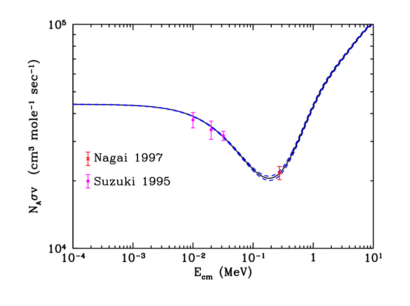
Knowing the $p(n,\gamma)d$ reaction is key in determining the end of the deuterium bottleneck and thus the onset of big bang nucleosynthesis. This radiative capture reaction is measured sparsely in the energy range of interest for BBN, $.01-1.0$ MeV. It is because of this lack of data that we must rely on a constrained R-matrix fit using elastic $p-p$, $n-p$ scattering, and both unpolarized and polarized $\gamma-d$ photo-disintegration data, in addition to the sparse $np$-capture data of Nagai 1997 nagai and Suzuki 1995 suzuki . We adopt the R-matrix calculation of Hale and Johnson (2003) hale , who have used the data discussed above to determine the $np$-capture cross section and its energy dependent uncertainties. This information was graciously provided by G. Hale upon private communication. This rate is now know to better than 2.5%, about a factor of 2 improvement over previous studies. We do not calculate a systematic error for this reaction.

III.1.3 $d(p,\gamma)\mbox{${}^{3}{\rm He}$}$

Figure 2: The reaction rate data for $d(p,\gamma)\mbox{${}^{3}{\rm He}$}$. The solid line represents the best fit, whilst the dashed the 1-sigma error bars. The data is shown with their respective 1-sigma error bars. The bottom panel shows the residual scattering in the data about our best fit, where our errors are set to $\pm 1$. The light curves are the Nollett and Burles nb00 best fit and $1\sigma$ errors.

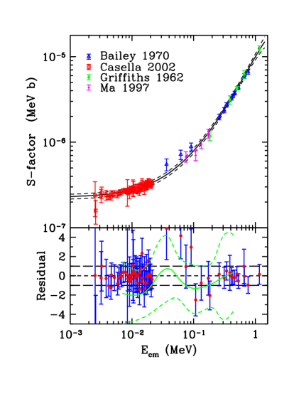
The $d(p,\gamma)\mbox{${}^{3}{\rm He}$}$ reaction is the first in a chain of reactions that rapidly burn deuterium after the deuterium bottleneck into ${}^{3}{\rm He}$ and eventually ${}^{4}{\rm He}$. There are few data sets for this reaction in the BBN energy range. We consider the data sets of Bailey (1970) dpgbailey , Griffiths (1962,1963) dpggriffiths , Ma (1997) dpgma , Schmid (1995,1996) dpgschmid and Casella (2002) dpgcasella . Some of these data sets warrant detailed consideration. The Casella data is the most recent measurement of this cross section and serves to anchor the low energy behavior of this reaction. This data has not been included in older analyses, only in this and two more recent BBN compilations by Cuoco et al cimm and Coc et al. cvdaa . It has been suggested that the 1963 Griffiths and 1970 Bailey experiments used incorrect stopping powers, and thus their low energy behavior is $\sim 15$ % too high dpgma ; dpgschmid . Since the Casella data dominates the low energy behavior of the cross section, inclusion of the Bailey data does not affect this region of the cross section, thus we find no reason to omit it from our analysis. The 1963 Griffiths data however, does not have a clear discussion of the normalization uncertainties, thus we exclude this data set from our analysis. The Schmid data sets suffer from poor energy resolution, with typical uncertainties in energy greater than 10%, which have not been included in their cross section errors. We thus exclude the Schmid data sets from the analysis. The inclusion of the new Casella data, greatly increases the accuracy of the cross section, when compared to previous analyses.

The discrepancy systematic error is $\delta_{disc}=0.0345$, the intrinsic normalization error is $\delta_{norm}=0.0528$ and the total systematic error is $\delta=0.0631$.

III.1.4 $d(d,n)\mbox{${}^{3}{\rm He}$}$

Figure 3: Same as fig. 2 but for $d(d,n)\mbox{${}^{3}{\rm He}$}$.

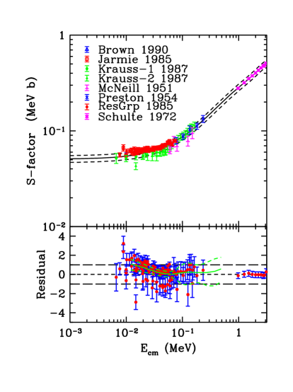
The $d(d,n)\mbox{${}^{3}{\rm He}$}$ reaction is the dominant deuterium sink during primordial nucleosynthesis. We consider the data sets of Brown (1990) brown , Krauss (1987) krauss , Ganeev (1958) ganeev , Arnold (1954) arnold , McNeill (1951) mcneill , Research Group (1985) resgrp , Preston (1954) preston , Jarmie (1985) ddn-jarmie and Schulte (1972) ddn-schulte . Of these data sets, inconsistancies in the Ganeev data set found on the NNDC website nndc , create difficulties when trying to separate systematic errors from the total errors presented (e.g. unphysical statistical errors), thus we exclude this data set. The Arnold data exists only as a smoothed data set. This smoothing will artificially increase this data set’s weight on the fit, thus we exclude this data set. The high energy Schulte data helps smoothly interpolate the gap between it and the low energy data. One may notice that the fitted curve falls below a majority of the data, a seemingly bad “chi-by-eye” fit. The eye is misleading in this case. Since we are treating the correlations between data points explicitly, it is important to understand its impact. As we determined in the previous section, the statistical uncertainty plays a larger role than the total uncertainty of a particular data point. When a data set has very small statistical uncertainties, it gets more weight when determining the fit. This is exactly what we are seeing here. Though the Brown and Research Group data have small normalization errors, their statistical errors are large when compared to the statistical uncertainties in the Krauss data, where $\sigma\mathrel{\mathchoice{\lower 3.6pt\vbox{\halign{$\mathsurround=0pt\displaystyle\hfil#\hfil$\cr<\crcr\sim\crcr}}}{\lower 3.6pt\vbox{\halign{$\mathsurround=0pt\textstyle\hfil#\hfil$\cr<\crcr\sim\crcr}}}{\lower 3.6pt\vbox{\halign{$\mathsurround=0pt\scriptstyle\hfil#\hfil$\cr<\crcr\sim\crcr}}}{\lower 3.6pt\vbox{\halign{$\mathsurround=0pt\scriptscriptstyle\hfil#\hfil$\cr<\crcr\sim\crcr}}}}1$ %. Even though the Krauss data has larger normalization uncertainties, its statistical errors are significantly smaller than other data sets, and thus the Krauss data dominates the low energy behavior of the fit. It is interesting to note that if we turn off the correlations between data points and adopt the total uncertainties as the representative errors, we reproduce the mean value of the Nollett and Burles curve.

The discrepancy systematic error is $\delta_{disc}=0.0369$, the intrinsic normalization error is $\delta_{norm}=0.0400$ and the total systematic error is $\delta=0.0544$.

III.1.5 $d(d,p)t$

Figure 4: Same as fig. 2 but for $d(d,p)t$.

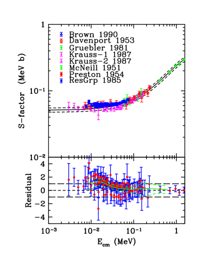
The $d(d,p)t$ reaction is very similar to its mirror $d(d,n)\mbox{${}^{3}{\rm He}$}$ reaction, both in shape and magnitude. We consider the data sets of Krauss (1987) krauss , Brown (1990) brown , Preston (1954) preston , Arnold (1954) arnold , Davenport (1953) ddp-davenport , Research Group (1985) resgrp , Ganeev (1958) ganeev , McNeill (1951) mcneill , and Gruebler (1981) ddp-gruebler . We exclude the data sets of Ganeev and Arnold for the same reasons as for the $d(d,n)\mbox{${}^{3}{\rm He}$}$ reaction. We again see the statistical uncertainties in the Krauss data pulling the fit below the Research Group and Brown data. Again, this is entirely due our explicit treatment of the correlations in the data. If we turn off the correlations and adopt the total uncertainty as the representative uncertainty, we again reproduce the mean value curve of Nollett and Burles.

The discrepancy systematic error is $\delta_{disc}=0.0487$, the intrinsic normalization error is $\delta_{norm}=0.0560$ and the total systematic error is $\delta=0.0742$.

III.1.6 $\mbox{${}^{3}{\rm He}$}(n,p)t$

Figure 5: Same as fig. 2 but for $\mbox{${}^{3}{\rm He}$}(n,p)t$.

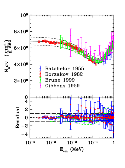
The $\mbox{${}^{3}{\rm He}$}(n,p)t$ reaction is responsible for the inter-conversion of mass 3 elements, maintaining an equilibrium relation between the two elements while this rate is fast when compared to the Hubble expansion rate. We consider the data sets of Brune (1999) 3np-brune , Costello (1970) 3np-costello , Coon (1950) 3np-coon , Gibbons (1959) gibbons , Macklin (1965) 3np-macklin , Batchelor (1955) 3np-batchelor , Borzakov (1982) 3np-borzakov and Alfimenkov (1980) 3np-alfimenkov . We exclude the Costello data because of poor energy resolution, the Coon and Macklin data because of little or no error information, and the Alfimenkov data because the reference was not available. There is a lot of data above 1 MeV for this reaction. In order to fit all of the data, we would need many fitting parameters. Since the energy range relevant for BBN is below 1 MeV, we do not use data above 1 MeV. As one can see, the fit is dominated by the Brune data.

The discrepancy systematic error is $\delta_{disc}=0.00703$, the intrinsic normalization error is $\delta_{norm}=0.0468$ and the total systematic error is $\delta=0.0473$.

III.1.7 $t(d,n)\mbox{${}^{4}{\rm He}$}$

Figure 6: Same as fig. 2 but for $t(d,n)\mbox{${}^{4}{\rm He}$}$.

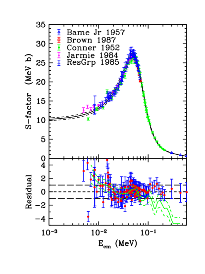
The $t(d,n)\mbox{${}^{4}{\rm He}$}$ reaction is a main production route to ${}^{4}{\rm He}$. We will consider the data sets of Allan (1951) tdn-allan , Argo (1952) tdn-argo , Arnold (1954) arnold , Bame Jr. (1957) tdn-bamejr , Brown (1987) tdn-brown , Conner (1952) tdn-conner , Davidenko (1957) tdn-davidenko , Jarmie (1984) tdn-jarmie and Research Group (1985) resgrp . We exclude the Allan and Argo data sets because of uncertain normalization error assignments, and the Davidenko data set because the reference was not available. We again exclude the Arnold data set because of their smoothing their data. The Conner data assumes the cross section is isotropic. This assumption is good up to energies of $E\sim 240$ keV, thus we exclude any Conner data that lie beyond this energy.

The discrepancy systematic error is $\delta_{disc}=0.0218$, the intrinsic normalization error is $\delta_{norm}=0.0401$ and the total systematic error is $\delta=0.0456$.

III.1.8 $\mbox{${}^{3}{\rm He}$}(d,p)\mbox{${}^{4}{\rm He}$}$

Figure 7: Same as fig. 2 but for $\mbox{${}^{3}{\rm He}$}(d,p)\mbox{${}^{4}{\rm He}$}$.

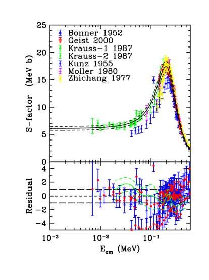
The $\mbox{${}^{3}{\rm He}$}(d,p)\mbox{${}^{4}{\rm He}$}$ reaction is also a main route for producing ${}^{4}{\rm He}$. We consider the data sets of Arnold (1954) arnold , Bonner (1952) 3dp-bonner , Geist (2000) 3dp-geist , Krauss (1987) krauss , Kunz (1955) 3dp-kunz , Moller (1980) 3dp-moller and Zhichang (1977) 3dp-zhichang . We exclude the Arnold data again, because of their smoothing the data.

The discrepancy systematic error is $\delta_{disc}=0.0268$, the intrinsic normalization error is $\delta_{norm}=0.0605$ and the total systematic error is $\delta=0.0662$.

III.1.9 $\mbox{${}^{3}{\rm He}$}(\alpha,\gamma)\mbox{${}^{7}{\rm Be}$}$

Figure 8: Same as fig. 2 but for $\mbox{${}^{3}{\rm He}$}(\alpha,\gamma)\mbox{${}^{7}{\rm Be}$}$.

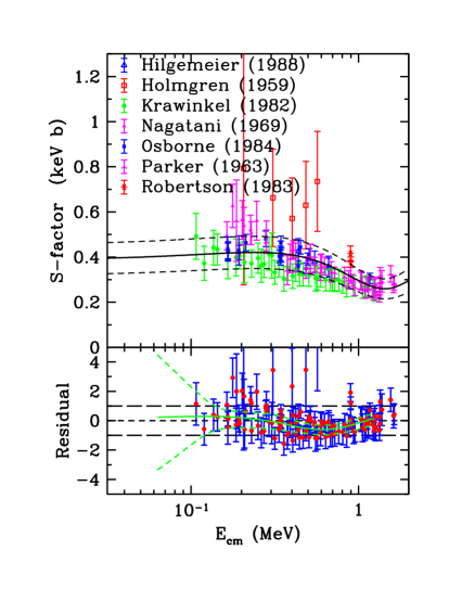
The $\mbox{${}^{3}{\rm He}$}(\alpha,\gamma)\mbox{${}^{7}{\rm Be}$}$ reaction is responsible for the production of ${}^{7}{\rm Li}$ in a high baryon density ($\eta\mathrel{\mathchoice{\lower 3.6pt\vbox{\halign{$\mathsurround=0pt\displaystyle\hfil#\hfil$\cr>\crcr\sim\crcr}}}{\lower 3.6pt\vbox{\halign{$\mathsurround=0pt\textstyle\hfil#\hfil$\cr>\crcr\sim\crcr}}}{\lower 3.6pt\vbox{\halign{$\mathsurround=0pt\scriptstyle\hfil#\hfil$\cr>\crcr\sim\crcr}}}{\lower 3.6pt\vbox{\halign{$\mathsurround=0pt\scriptscriptstyle\hfil#\hfil$\cr>\crcr\sim\crcr}}}}3\times 10^{-10}$) universe. Its uncertainty dominates the prediction of the ${}^{7}{\rm Li}$ abundance prediction. We consider the data sets of Holmgren (1959) holmgren , Parker (1963) 3ag-parker , Nagatani (1969) 3ag-nagatani , Krawinkel (1982) 3ag-krawinkel , Robertson (1983) 3ag-robertson , Hilgemeier (1988) 3ag-hilgemeier and Osborne (1984) 3ag-osborne . Following the suggestion of Hilgemeier, we renormalize the Krawinkel data by the factor 1.4, correcting the helium gas density.

The discrepancy systematic error is $\delta_{disc}=0.1482$, the intrinsic normalization error is $\delta_{norm}=0.0814$ and the total systematic error is $\delta=0.1691$.

This reaction is also very important for stellar physics, in particular neutrino production. The low energy behavior of this reaction rate determines the flux of ${}^{7}{\rm Be}$ and ${}^{8}{\rm B}$ neutrinos coming from the Sun. We believe it is inappropriate to base the low energy value on an average of extrapolated points, and recommend our adopted method of a global analysis of the data and its uncertainties and then extrapolating a low energy value. We get a value of $S_{34}(0)=(1.0\pm 0.169)(0.386\pm 0.020)=0.386\pm 0.068$ keV b for the astrophysical $S$-factor. This is significantly lower than the values determined by Adelberger et al. $S_{34}^{\rm Adlb}=0.53\pm 0.05$ keV b Adelberger , the NACRE collaboration $S_{34}^{\rm nacre}=0.54\pm 0.09$ keV b nacre and the Cyburt, Fields and Olive cfo1 renormalized NACRE rate $S_{34}^{\rm CFO}=0.50\pm 0.05$ keV b, though all determinations are based primarily on the same data. The Osborne data dominates the fit at low energy, causing the downward turn of the $S$-factor. This turn is also seen in the Nollett and Burles compilation nb00 . The model independent approach adopted in this work and in the work of Nollett and Burles should not be used for extrapolation, as these methods are meant to describe the data alone and thus are only valid where data exists. However, the inclusion of any theory fitting this data will still have to include the systematic errors similar to the ones discussed in this work. More measurements with $E\mathrel{\mathchoice{\lower 3.6pt\vbox{\halign{$\mathsurround=0pt\displaystyle\hfil#\hfil$\cr<\crcr\sim\crcr}}}{\lower 3.6pt\vbox{\halign{$\mathsurround=0pt\textstyle\hfil#\hfil$\cr<\crcr\sim\crcr}}}{\lower 3.6pt\vbox{\halign{$\mathsurround=0pt\scriptstyle\hfil#\hfil$\cr<\crcr\sim\crcr}}}{\lower 3.6pt\vbox{\halign{$\mathsurround=0pt\scriptscriptstyle\hfil#\hfil$\cr<\crcr\sim\crcr}}}}0.5$ MeV will be able to more precisely determine $S_{34}(0)$.

III.1.10 $t(\alpha,\gamma)\mbox{${}^{7}{\rm Li}$}$

Figure 9: Same as fig. 2 but for $t(\alpha,\gamma)\mbox{${}^{7}{\rm Li}$}$.

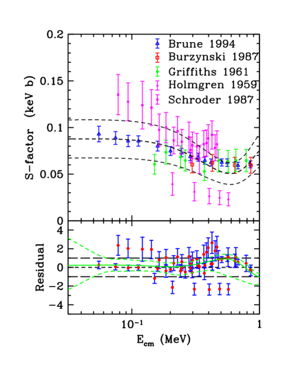
The $t(\alpha,\gamma)\mbox{${}^{7}{\rm Li}$}$ reaction is important for ${}^{7}{\rm Li}$ production in a low baryon density ($\eta\mathrel{\mathchoice{\lower 3.6pt\vbox{\halign{$\mathsurround=0pt\displaystyle\hfil#\hfil$\cr<\crcr\sim\crcr}}}{\lower 3.6pt\vbox{\halign{$\mathsurround=0pt\textstyle\hfil#\hfil$\cr<\crcr\sim\crcr}}}{\lower 3.6pt\vbox{\halign{$\mathsurround=0pt\scriptstyle\hfil#\hfil$\cr<\crcr\sim\crcr}}}{\lower 3.6pt\vbox{\halign{$\mathsurround=0pt\scriptscriptstyle\hfil#\hfil$\cr<\crcr\sim\crcr}}}}3\times 10^{-10}$) universe. Its uncertainty dominates the theory prediction of ${}^{7}{\rm Li}$’s abundance here. We consider the data sets of Brune (1994) tag-brune , Burzynski (1987) tag-burzynski , Griffiths (1961) tag-griffiths , Holmgren (1959) holmgren , Schroder (1987) tag-schroder and Utsunomiya (1990) tag-utsunomiya . We exclude the Utsunomiya data set because of the lack of a normalization error discussion. Smith, Kawano and Malaney skm and Nollett and Burles nb00 make the point that these Coulomb-breakup measurements are not yet reliable as this process is not yet completely understood, thus making the case for new experiments to be performed with $E\mathrel{\mathchoice{\lower 3.6pt\vbox{\halign{$\mathsurround=0pt\displaystyle\hfil#\hfil$\cr<\crcr\sim\crcr}}}{\lower 3.6pt\vbox{\halign{$\mathsurround=0pt\textstyle\hfil#\hfil$\cr<\crcr\sim\crcr}}}{\lower 3.6pt\vbox{\halign{$\mathsurround=0pt\scriptstyle\hfil#\hfil$\cr<\crcr\sim\crcr}}}{\lower 3.6pt\vbox{\halign{$\mathsurround=0pt\scriptscriptstyle\hfil#\hfil$\cr<\crcr\sim\crcr}}}}0.2$ MeV.

It is clear that the Holmgren and Schroder data are far from the best fit curve, outside of their assigned normalization errors. The visible discrepancy is forcing the sytematic error to be quite large. The Holmgren data also pulls the $S$-factor fit down at $E\sim 0.6$ MeV. If reason, other than the visible discrepancy exists to exclude these data, the fit would be dominated by the high precision Brune data with an overall 6% normalization error.

The discrepancy systematic error is $\delta_{disc}=0.1788$, the intrinsic normalization error is $\delta_{norm}=0.1468$ and the total systematic error is $\delta=0.2313$.

III.1.11 $\mbox{${}^{7}{\rm Be}$}(n,p)\mbox{${}^{7}{\rm Li}$}$

Figure 10: Same as fig. 2 but for $\mbox{${}^{7}{\rm Be}$}(n,p)\mbox{${}^{7}{\rm Li}$}$.

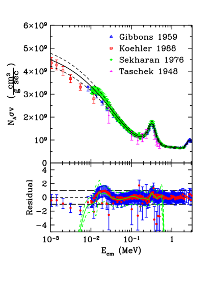
The $\mbox{${}^{7}{\rm Be}$}(n,p)\mbox{${}^{7}{\rm Li}$}$ reaction is responsible for the inter-conversion of mass 7 elements at high baryon density ($\eta\mathrel{\mathchoice{\lower 3.6pt\vbox{\halign{$\mathsurround=0pt\displaystyle\hfil#\hfil$\cr>\crcr\sim\crcr}}}{\lower 3.6pt\vbox{\halign{$\mathsurround=0pt\textstyle\hfil#\hfil$\cr>\crcr\sim\crcr}}}{\lower 3.6pt\vbox{\halign{$\mathsurround=0pt\scriptstyle\hfil#\hfil$\cr>\crcr\sim\crcr}}}{\lower 3.6pt\vbox{\halign{$\mathsurround=0pt\scriptscriptstyle\hfil#\hfil$\cr>\crcr\sim\crcr}}}}3\times 10^{-10}$). This reaction has only one data set in the exoergic direction. The data set of Koehler (1988) 7np-koehler . This data set does not extend very far into the energy range of interest for BBN. We must rely on the data for the endoergic reverse reaction, $\mbox{${}^{7}{\rm Li}$}(p,n)\mbox{${}^{7}{\rm Be}$}$. We consider the data sets of Gibbons (1959) gibbons , Sekharan (1976) 7np-sekharan and Taschek (1948) 7np-taschek . We use the principal of detailed balance to transform the $\mbox{${}^{7}{\rm Li}$}(p,n)\mbox{${}^{7}{\rm Be}$}$ data into $\mbox{${}^{7}{\rm Be}$}(n,p)\mbox{${}^{7}{\rm Li}$}$ data. Using the $Q$-value from Audi and Wapstra (1995) audi available at the US Nuclear Data Program website USNDP , $Q=1.644168\pm 0.000668$ MeV. We ignore the lowest energy points derived from the reverse rate as they are sensitive to the precise value of $Q$, ignoring values that change significantly when $Q$ is varied within its uncertainties. We should note that the Koehler data extends down to well below 1 eV, we choose not to show the data as its roughly constant and to emphasize the energy range important for primordial nucleosynthesis.

The discrepancy systematic error is $\delta_{disc}=0.0159$, the intrinsic normalization error is $\delta_{norm}=0.0448$ and the total systematic error is $\delta=0.0475$.

III.1.12 $\mbox{${}^{7}{\rm Li}$}(p,\alpha)\mbox{${}^{4}{\rm He}$}$

Figure 11: Same as fig. 2 but for $\mbox{${}^{7}{\rm Li}$}(p,\alpha)\mbox{${}^{4}{\rm He}$}$. Also shown is the $e$-screening corrected $S$-factor and its uncertainty.

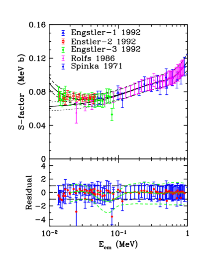
The $\mbox{${}^{7}{\rm Li}$}(p,\alpha)\mbox{${}^{4}{\rm He}$}$ reaction is the dominant destruction channel of ${}^{7}{\rm Li}$ at low baryon densities ($\eta\mathrel{\mathchoice{\lower 3.6pt\vbox{\halign{$\mathsurround=0pt\displaystyle\hfil#\hfil$\cr<\crcr\sim\crcr}}}{\lower 3.6pt\vbox{\halign{$\mathsurround=0pt\textstyle\hfil#\hfil$\cr<\crcr\sim\crcr}}}{\lower 3.6pt\vbox{\halign{$\mathsurround=0pt\scriptstyle\hfil#\hfil$\cr<\crcr\sim\crcr}}}{\lower 3.6pt\vbox{\halign{$\mathsurround=0pt\scriptscriptstyle\hfil#\hfil$\cr<\crcr\sim\crcr}}}}3\times 10^{-10}$). We consider the data sets of Engstler (1992) 7pa-engstler , Harmon (1989) 7pa-harmon , Lee (1969) 7pa-lee , Rolfs (1986) 7pa-rolfs and Spinka (1971) 7pa-spinka . We exclude the Harmon data because it is based on a measurement relative to $\mbox{${}^{6}{\rm Li}$}(p,\alpha)\mbox{${}^{3}{\rm He}$}$ at energies $E\mathrel{\mathchoice{\lower 3.6pt\vbox{\halign{$\mathsurround=0pt\displaystyle\hfil#\hfil$\cr>\crcr\sim\crcr}}}{\lower 3.6pt\vbox{\halign{$\mathsurround=0pt\textstyle\hfil#\hfil$\cr>\crcr\sim\crcr}}}{\lower 3.6pt\vbox{\halign{$\mathsurround=0pt\scriptstyle\hfil#\hfil$\cr>\crcr\sim\crcr}}}{\lower 3.6pt\vbox{\halign{$\mathsurround=0pt\scriptscriptstyle\hfil#\hfil$\cr>\crcr\sim\crcr}}}}150$ keV by Shinozuka et al (1979) 7pa-shinozuka . All but 3 points lie below this energy range, thus this measurement relative to $\mbox{${}^{6}{\rm Li}$}(p,\alpha)\mbox{${}^{3}{\rm He}$}$ is not valid at these energies. One may consider using the 3 points that are measured at appropriate energies, but it does not change our fit significantly. We also exclude the Lee data set as the reference was unavailable.

This reaction has the largest Gamow energy of all the reactions we consider, and thus is the most susceptible to electron screening effects. In fact, the low energy behavior of this reaction is modified by electron-screening effects in the experimental set-up. This behavior can be parameterized as $\sigma_{\rm exp}(E)=\sigma_{\rm bare}(E+U_{e})$, relating the experimentally measured cross section to the bare nuclear cross section (i.e. no electron screening), where $U_{e}$ is the screening potential 7np-escreening . Where $U_{e}$ is a measure of how much the Coulomb barrier has been reduced due to electrons screening the bare nucleus (e.g. ${}^{7}{\rm Li}$). For the experiments that screening is important (i.e. Engstler), $U_{e}=245\pm 45$ eV is found to be the best fit. This agrees with the determinations of Engstler et al., who find $U_{e}=300\pm 160$ eV using an approximation of the $e$-screening correction to the observed cross section shown above. Englster used the high energy data to determine the best fit, and then extrapolate this to determine the screening potential. We have fit all the data, including the electron screening potential self-consistantly.

The discrepancy systematic error is $\delta_{disc}=0.0194$, the intrinsic normalization error is $\delta_{norm}=0.0769$ and the total systematic error is $\delta=0.0793$. There is an additional energy dependent systematic error induced because of our electron screening correction. This can be well accounted for by:

$$\delta_{e-scr}=0.02015\left(\frac{\sigma_{U_{e}}}{45\ {\rm eV}}\right)\exp{(-15.34E)},$$ (35)

again added in quadrature with the other systematics.

III.2 Thermal Rates

For the BBN temperature range, Maxwell-Boltzmann phase-space distributions are an excellent choice for baryons (eqn. 25) and the thermal rates become,

$$\lambda=N_{A}\left(\frac{8}{\pi\mu(kT)^{3}}\right)^{1/2}\int_{0}^{\infty}\sigma(E)E\exp{\left(-\frac{E}{kT}\right)}dE,$$ (36)

where $\sigma(E)$ is the cross section, not the standard deviation. For neutron induced reactions, using eqn. 32, we find

$$\lambda=\frac{2}{\sqrt{\pi}(kT)^{3/2}}\int_{0}^{\infty}R(E)E^{1/2}\exp{\left(-\frac{E}{kT}\right)}dE;$$ (37)

and for charge induced reactions, using eqn. 33, we find

$$\lambda=N_{A}\left(\frac{8}{\pi\mu(kT)^{3}}\right)^{1/2}\int_{0}^{\infty}S(E)\exp{\left[-\frac{E}{kT}-\left(\frac{E_{g}}{E}\right)^{1/2}\right]}dE.$$ (38)

It is trivial to determine the weighting functions with these relations. For the neutron- and charge- induced reactions the respective weighting functions are:

$$W(E,T) = \frac{2}{\sqrt{\pi}(kT)^{3/2}}E^{1/2}\exp{\left(-\frac{E}{kT}\right)}$$ (39)

$$W(E,T) = N_{A}\left(\frac{8}{\pi\mu(kT)^{3}}\right)^{1/2}\exp{\left[-\frac{E}{kT}-\left(\frac{E_{g}}{E}\right)^{1/2}\right]}.$$ (40)

After these integrals are performed numerically, we must find some representation of these thermal rates to implement into the BBN code. We will look at some cases in which the above integrals can be done analytically. This will ultimately guide us in determining the functional forms for these rates.

Typically, neutron induced reactions follow the $v^{-1}$ behavior noted in the previous chapter and are particularly smooth over the data energy range coverage. Thus a simple polynomial in $E^{1/2}$ will generally suffice. In this case, the integral can be performed analytically and the numerical integration serves as a test of the integrator.

Most of the reactions are non-resonant charge induced reactions. In this case the integral cannot be done analytically, particularly at the temperature ranges relevant for BBN. In order to understand the reason for this and gain some insight for a possible functional form, we will look at the case where the temperature is much smaller than the Gamow energy, $kT\ll E_{g}$. We would like to turn the weighting function in eqn 40 into something more familiar, like a gaussian. To do this, we Taylor expand the argument of the exponent, about some energy $E_{0}$, defined such that the first derivative with respect to energy is zero at $E_{0}$. Doing this we find, $E_{0}/E_{g}=(kT/2E_{g})^{2/3}$. Also needed for this analysis is the width of this gaussian, which we can find by evaluating the second derivative of the exponent argument at $E_{0}$. We find, $\sigma_{0}/E_{g}=2/\sqrt{3}(kT/2E_{g})^{5/6}$. The relevant perturbative parameter is the ratio of this width to effective energy, $\sigma_{0}/E_{0}=(32kT/27E_{g})^{1/6}$. In order for this gaussian approximation of the integrand to converge, the width must be much smaller than the effective energy. Not only does this demand $kT\ll E_{g}$, but since the power is small $(kT/E_{g})^{1/6}$ must be small. To get 10% convergence, $kT\mathrel{\mathchoice{\lower 3.6pt\vbox{\halign{$\mathsurround=0pt\displaystyle\hfil#\hfil$\cr<\crcr\sim\crcr}}}{\lower 3.6pt\vbox{\halign{$\mathsurround=0pt\textstyle\hfil#\hfil$\cr<\crcr\sim\crcr}}}{\lower 3.6pt\vbox{\halign{$\mathsurround=0pt\scriptstyle\hfil#\hfil$\cr<\crcr\sim\crcr}}}{\lower 3.6pt\vbox{\halign{$\mathsurround=0pt\scriptscriptstyle\hfil#\hfil$\cr<\crcr\sim\crcr}}}}10^{-6}E_{g}$, which is well below the range relevant for BBN. However, if we continue, we find that the rate transforms into:

$$\lambda=N_{A}\left(\frac{8}{\mu\pi}\right)^{1/2}\frac{\sigma_{0}}{(kT)^{3/2}}\exp{\left[-\left(\frac{27E_{g}}{4kT}\right)^{1/3}\right]}S_{eff}(E_{0}).$$ (41)

If $S(E)$ is taken to be a polynomial in $E$, then $S_{eff}(E_{0})$ is a polynomial in $(\sigma_{0}/E_{0})^{2}\propto kT^{1/3}$, where only the even powers of our perturbative parameter appear due to the symmetry of the gaussian. We adopt this form, allowing the order of the polynomial describing $S_{eff}(E_{0})$ to vary as needed until an accurate fit is reached. Reactions with broad resonances modify the above form, with the Breit-Wigner form, with $E=E_{0}$;

$$\lambda=N_{A}\left(\frac{8}{\mu\pi}\right)^{1/2}\frac{\sigma_{0}}{(kT)^{3/2}}\exp{\left[-\left(\frac{27E_{g}}{4kT}\right)^{1/3}\right]}\frac{S_{eff}(E_{0})}{1+((E_{0}-E_{R})/\Gamma_{R}/2)^{2}},$$ (42)

where $E_{R}$ and $\Gamma_{R}$ are the resonance parameters and $S_{eff}(E_{0})$ is a polynomial in powers of $kT^{1/3}$.

Reactions with narrow resonances are typically the sum of a non-resonant piece and a Breit-Wigner form. Since the resonance is narrow, we can treat the Breit-Wigner form as a delta function. In the case of a neutron induced reaction, the resonant part of the rate becomes:

$$\lambda_{res}=\sqrt{\pi}\frac{\Gamma_{R}E_{R}^{1/2}}{(kT)^{3/2}}R(E_{R})\exp{(-E_{R}/kT)}.$$ (43)

We wish to reiterate here, that the cross section fits and their energy dependent uncertainties are numerically integrated. These exact results are subsequently cast into a usable form, fit to one of the forms mentioned above to within 0.1%.

In thermonuclear rate compilations, such as this one, it is important to realize that most compilations rely on the same experimental data to derive their representations. Because of this, they must generally agree with each other over the range of validity. This range is shown it table 2. The limits are solely based on the maximum energy of the data used ($kT_{max}\sim E_{max}/3$).

Table 2: This table shows to what maximum temperature each thermal rate is valid for. This is solely due to the data used in the analysis. Also shown are the systematic errors.

Reactions	$T_{max}$ ($10^{9}$ K)	$\delta_{disc}$	$\delta_{norm}$	$\delta_{tot}$
$p(n,\gamma)d$	100	N.A.	N.A.	N.A.
$d(p,\gamma)\mbox{${}^{3}{\rm He}$}$	3.9	0.0345	0.0528	0.0631
$d(d,n)\mbox{${}^{3}{\rm He}$}$	12.5	0.0369	0.0400	0.0544
$d(d,p)t$	5.8	0.0487	0.0560	0.0742
$\mbox{${}^{3}{\rm He}$}(n,p)t$	3.9	0.0071	0.0468	0.0473
$t(d,n)\mbox{${}^{4}{\rm He}$}$	2.3	0.0218	0.0401	0.0456
$\mbox{${}^{3}{\rm He}$}(d,p)\mbox{${}^{4}{\rm He}$}$	2.3	0.0268	0.0605	0.0662
$\mbox{${}^{3}{\rm He}$}(\alpha,\gamma)\mbox{${}^{7}{\rm Be}$}$	7.8	0.1482	0.0814	0.1691
$t(\alpha,\gamma)\mbox{${}^{7}{\rm Li}$}$	3.9	0.1788	0.1468	0.2313
$\mbox{${}^{7}{\rm Be}$}(n,p)\mbox{${}^{7}{\rm Li}$}$	11.7	0.0159	0.0448	0.0475
$\mbox{${}^{7}{\rm Li}$}(p,\alpha)\mbox{${}^{4}{\rm He}$}$	3.9	0.0194	0.0769	0.0793

We first compare to the BBN reaction rate standard, Smith, Kawano and Malaney (1993) skm . As we see from fig. 12, there is overall agreement with our compilation and theirs. The curves tend to diverge at high temperature, where there is no data pinning down the high energy behavior. The disagreement with the rate for $d(p,\gamma)\mbox{${}^{3}{\rm He}$}$ is almost entirely due to the use and exclusion of different data sets. The disagreement at low temperatures for $\mbox{${}^{7}{\rm Be}$}(n,p)\mbox{${}^{7}{\rm Li}$}$, is most likely due to their taking a minimum energy when integrating this rate ($E_{min}=1$ keV). We cannot compare directly to Nollett and Burles (2000) nb00 as they do not present thermal rates, but differences are attributable to the differences in cross section representations already discussed. The “wiggles” seen in $t(d,n)\mbox{${}^{4}{\rm He}$}$, $\mbox{${}^{3}{\rm He}$}(d,p)\mbox{${}^{4}{\rm He}$}$ and $\mbox{${}^{7}{\rm Be}$}(n,p)\mbox{${}^{7}{\rm Li}$}$ are due to the slightly different values adopted for the resonance parameters of each reaction.

Figure 12: The thermal reaction rate residuals of the Smith, Kawano & Malaney (1993) skm compilation plotted against temperature in units of $10^{9}$ K. The solid line shows how their mean value compares to this compilations mean value. The dashed lines correspond with the $1\sigma$ errors.

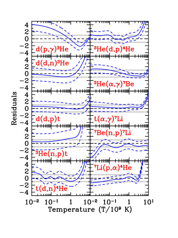
We now compare to the work of Cyburt, Fields and Olive (2001) cfo1 , which used renormalized NACRE rates and an estimate of the errors. Again, since these compilations are based on most of the same nuclear data the rates should be similar, as seen in fig. 13. An interesting point is that for a majority of reactions, the Cyburt, Fields and Olive error budget underestimates the errors, compared to this work. The intrinsic normalization error we have included is typically as important as the discrepancy systematic error, which Cyburt, Fields and Olive assumed to dominate the error budget. Again the high temperature portion of the curves tend to diverge, as there is no data pinning down the high energy behavior. We point out that the $d(p,\gamma)\mbox{${}^{3}{\rm He}$}$ rate as it is systematically lower than our rate. This is entirely due to the NACRE collaboration’s inclusion of data we have excluded. Also evident are the differences in the $d(d,n)\mbox{${}^{3}{\rm He}$}$ and $d(d,p)t$ rates, where our compilation falls below the fits adopted by Cyburt, Fields and Olive. The differences between this compilation and others for these rates, is that we have included the correlations between data points. It is for this reason, that the low energy data that has small statistical, but large total error is dominating the fits, pulling the low energy cross section down slightly.

Figure 13: The thermal reaction rate residuals of the Cyburt, Fields & Olive (2001) cfo1 reanalysis of NACRE nacre plotted against temperature in units of $10^{9}$ K. The solid line shows how their mean value compares to this compilations mean value. The dashed lines correspond with the $1\sigma$ errors.

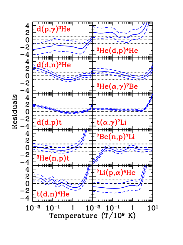
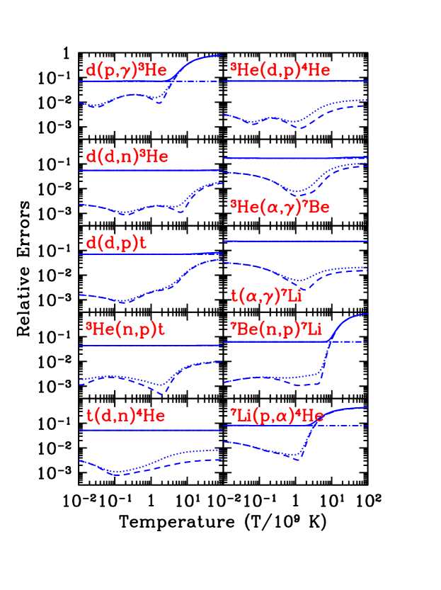
The overall agreement between different rate compilations is quite reassuring. The biggest advantage to our compilation is we have explicit treatments for dealing with correlated data, and estimating systematic errors. These systematic errors dominate over the statistical uncertainties in all cases, for the temperature range important for BBN, $T\sim(0.5-1.2)\times 10^{9}$ K as seen in fig. 14. Properly treating the correlation between fitting parameters when propagating the cross section fits into thermal rates has a noticeable reduction in the statistical uncertainties. This reduction is maximized when there is a cross over between terms in the fit polynomial, when one term goes from being dominant to being sub-dominant and vice versa. It is also reassuring to see the statistical uncertainty become the dominant contribution to the error at high temperature or energies, where there is no data.

Figure 14: The thermal reaction rate relative errors for the 10 reactions fitted in this compilation. The dashed and dotted curves are the thermally averaged statistical errors with and without treating the energy correlations. The dashed-dotted curve shows the total systematic errors, and the solid curve shows the total thermal error.

III.3 Light Element Predictions

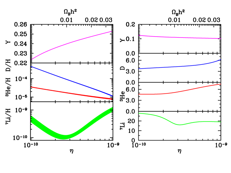
Adopting the thermonuclear reaction rates discussed in the previous section, we discuss their impact on BBN predictions and on the general concordance of the BBN predictions with the light element observations and the CMB. Shown in figure 15 are the light element abundance predictions and their percent errors using this work’s nuclear compilation.

Figure 15: Shown in the left panel are the light element predictions using this works nuclear rate compilation and uncertainties. The mass fraction of ${}^{4}{\rm He}$ ($Y_{p}$) and the mole fractions, ${\rm D/H}$, $\mbox{${}^{3}{\rm He}$}/{\rm H}$ and $\mbox{${}^{7}{\rm Li}$}/{\rm H}$ are plotted against the baryon-to-photon ratio. The width of each curve represents the 1 $\sigma$ errors in the light element predictions. The right panel shows the relative uncertainties in percent of the light element predictions.

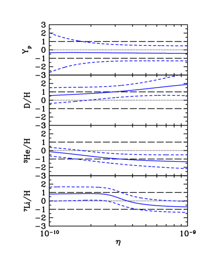
Before we examine the concordance between this compilation’s predictions and observations, we should verify the agreement of previous compilations and qualify their differences. As has been discussed in previous chapters, the BBN compilations of Smith, Kawano and Malaney skm , Nollett and Burles nb00 and Cyburt, Fields and Olive cfo1 , should all roughly agree as they are largely based on the same nuclear data. Any differences in their predictions will arise entirely from each compilation’s derivation of reaction rates and their uncertainties, and the data each uses.

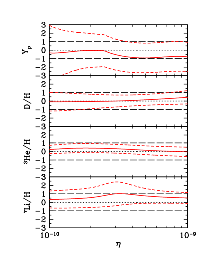
Since Cyburt, Fields and Olive and Nollett and Burles both compare directly to Smith, Kawano and Malaney showing rough agreement, we choose to compare only to the former two compilations. Plotted in figure 16 is the residual between Cyburt, Fields and Olive cfo1 and this compilation, where zero and $\pm 1$ represent the means and standard deviations of this compilation. The ${}^{4}{\rm He}$ mass fraction ($Y_{p}$) is in good agreement with this compilation. The ${}^{4}{\rm He}$ abundance error is slightly increased due to the inclusion of the uncertainty in Newtion’s G_N. This compilations treatment of the data, leads to differences for the D, ${}^{3}{\rm He}$ and ${}^{7}{\rm Li}$ yields. On the high $\eta$ side ($\eta\mathrel{\mathchoice{\lower 3.6pt\vbox{\halign{$\mathsurround=0pt\displaystyle\hfil#\hfil$\cr>\crcr\sim\crcr}}}{\lower 3.6pt\vbox{\halign{$\mathsurround=0pt\textstyle\hfil#\hfil$\cr>\crcr\sim\crcr}}}{\lower 3.6pt\vbox{\halign{$\mathsurround=0pt\scriptstyle\hfil#\hfil$\cr>\crcr\sim\crcr}}}{\lower 3.6pt\vbox{\halign{$\mathsurround=0pt\scriptscriptstyle\hfil#\hfil$\cr>\crcr\sim\crcr}}}}3\times 10^{-10}$) the changes are due to the $d(p,\gamma)\mbox{${}^{3}{\rm He}$}$ reaction. The new cross section is larger than the one determined by the NACRE-based compilation nacre of Cyburt, Fields and Olive, causing a subsequent drop in D yields with a simultaneous jump in ${}^{3}{\rm He}$ and ${}^{7}{\rm Li}$ yields. For low values of $\eta$, only the mean value of ${}^{7}{\rm Li}$ is significantly different. This is due entirely to a slightly lower cross section for the $t(\alpha,\gamma)\mbox{${}^{7}{\rm Li}$}$ reaction used here. The errors of the Cyburt, Fields and Olive compilation are generally smaller than this compilation’s errors. This is due to the fact that this compilation has an additional intrinsic normalization error added in quadrature with the discrepancy normalization error.

Figure 16: This figure shows the difference between light element yields using this compilation and that of Cyburt, Fields and Olive cfo1 . The solid and short-dashed curves show the Cyburt, Fields and Olive yield means and standard deviations with respect to this compilation’s means and standard deviations, seen here as zero and $\pm 1$, respectively.

Similarly, plotted in figure 17 is the residual between Nollett and Burles nb00 and this compilation. The central values of the abundance yields are in good agreement. The most noticeable difference is in the ${}^{7}{\rm Li}$ yields, with this compilation having slightly lower values. The high $\eta$ difference is due to differences in the reactions $d(p,\gamma)\mbox{${}^{3}{\rm He}$}$ and $\mbox{${}^{3}{\rm He}$}(d,p)\mbox{${}^{4}{\rm He}$}$, while on the low $\eta$ side the differences are primarily due to the reaction $t(d,n)\mbox{${}^{4}{\rm He}$}$. The errors of Nollett and Burle’s compilation are comparable, but generally smaller than this compilation’s errors, because of the statistical nature of their errors. The larger ${}^{4}{\rm He}$ error is due to the larger uncertainty in the neutron lifetime adopted by Nollett and Burles.

Figure 17: This figure shows the difference between light element yields using this compilation and that of Nollett and Burles nb00 . The solid and short-dashed curves show the Nollett and Burles yield means and standard deviations with respect to this compilation’s means and standard deviations, seen here as zero and $\pm 1$, respectively.

It is reassuring that this new BBN nuclear compilation agrees quite well with the previous studies of Smith, Kawano and Malaney skm , Nollett and Burles nb00 and Cyburt, Fields and Olive cfo1 , as well as the two more recent calculations by Cuoco et al. cimm and Coc et al. cvdaa , though the new compilations do not present rate representations that can be compared directly. This work’s rigorous treatment of systematic uncertainties also suggests that these previous works may have underestimated the true error budget in the light element abundance predictions. This comparison also suggests where new nuclear data will be most useful. To illustrate this point, scalings are created that explicitly show how the baryon-to-photon ratio $\eta$, Newton’s G and the reaction rates affect the light element abundance predictions. These scalings are calculated numerically, by finding the logarithmic derivatives of the light element abundance predictions with respect to parameters and key reaction rates, relative to a fiducial model where $\eta=6.14\times 10^{-10}$ flsv . They can be used to either predict light element abundances or propagate uncertainties, but these scalings are only approximate and will change for models with $\eta$ very far from its fiducial value. We use them here, only to discuss how BBN’s predictions depend on the various inputs. The nuclear reactions are parametrized here through $R_{i}$, where $i$ refers to the subsection number assignment for that reaction in sect. III.1 (i.e. $R_{2}$, $R_{4}$, and $R_{5}$ correspond with the $p(n,\gamma)d$, $d(d,n)\mbox{${}^{3}{\rm He}$}$, and $d(d,p)t$ reactions respectively). The $R_{i}$ can be thought of as reaction normalizations, such that the current compilation is $R_{i}=1.0$. The scalings are:

$$Y_{p} = 0.24849\left(\frac{10^{10}\eta}{6.14}\right)^{\!\!0.39}\!\!\left(\frac{\tau_{n}}{\tau_{n,0}}\right)^{\!\!0.72}\!\!\left(\frac{{\rm G}_{N}}{{\rm G}_{N,0}}\right)^{\!\!0.35}\!\!\!\!\!\!R_{4}^{0.006}R_{5}^{0.005}R_{2}^{0.005}$$ (44)

$$10^{5}\frac{\rm D}{\rm H} = 2.558\left(\frac{10^{10}\eta}{6.14}\right)^{\!\!-1.62}\!\!\!\left(\frac{\tau_{n}}{\tau_{n,0}}\right)^{\!\!0.41}\!\!\left(\frac{{\rm G}_{N}}{{\rm G}_{N,0}}\right)^{\!\!0.95}\!\!\!\!\!\!R_{4}^{-0.55}R_{5}^{-0.45}R_{3}^{-0.32}R_{2}^{-0.20}$$ (45)

$$10^{6}\frac{\mbox{${}^{3}{\rm He}$}}{\rm H} = 10.086\left(\frac{10^{10}\eta}{6.14}\right)^{\!\!-0.59}\!\!\left(\frac{\tau_{n}}{\tau_{n,0}}\right)^{\!\!0.15}\!\!\left(\frac{{\rm G}_{N}}{{\rm G}_{N,0}}\right)^{\!\!0.34}\!\!\!\!\!\!R_{8}^{-0.77}R_{3}^{0.38}R_{5}^{-0.25}R_{4}^{-.20}R_{6}^{-0.17}R_{2}^{0.08}$$ (46)

$$10^{10}\frac{\mbox{${}^{7}{\rm Li}$}}{\rm H} = 4.364\left(\frac{10^{10}\eta}{6.14}\right)^{\!\!2.12}\!\!\left(\frac{\tau_{n}}{\tau_{n,0}}\right)^{\!\!0.44}\!\!\left(\frac{{\rm G}_{N}}{{\rm G}_{N,0}}\right)^{\!\!-0.72}\!\!\!\!\!\!R_{2}^{1.34}R_{9}^{0.96}R_{8}^{-0.76}R_{11}^{-0.71}R_{4}^{0.71}R_{3}^{0.59}R_{6}^{-0.27}.$$ (47)

As clearly seen in the scalings, $Y_{p}$ is dominated by the neutron mean lifetime and Newton’s G_N, while the reactions $d(d,n)\mbox{${}^{3}{\rm He}$}$, $d(d,p)t$ and $p(n,\gamma)d$ only slightly change the predictions. The dramatic drop in sensitivity (scaling powers $\sim 0.5$ to $\sim 0.005$) is seen in the other light element scalings, meaning those reactions do not contribute significantly to the overall theory predicions. Thus, for brevity these reactions are left out of the scalings for D, ${}^{3}{\rm He}$ and ${}^{7}{\rm Li}$. For an accurate D prediction, $d(d,n)\mbox{${}^{3}{\rm He}$}$ and $d(d,p)t$ are key, with $d(p,\gamma)\mbox{${}^{3}{\rm He}$}$ following close behind. ${}^{3}{\rm He}$ is the least sensitive to which nuclear compilation is used, though improvements in its prediction propagates into an improved ${}^{7}{\rm Li}$ prediction. For high baryon densities ($\eta\mathrel{\mathchoice{\lower 3.6pt\vbox{\halign{$\mathsurround=0pt\displaystyle\hfil#\hfil$\cr>\crcr\sim\crcr}}}{\lower 3.6pt\vbox{\halign{$\mathsurround=0pt\textstyle\hfil#\hfil$\cr>\crcr\sim\crcr}}}{\lower 3.6pt\vbox{\halign{$\mathsurround=0pt\scriptstyle\hfil#\hfil$\cr>\crcr\sim\crcr}}}{\lower 3.6pt\vbox{\halign{$\mathsurround=0pt\scriptscriptstyle\hfil#\hfil$\cr>\crcr\sim\crcr}}}}3\times 10^{-10}$), the reactions $\mbox{${}^{3}{\rm He}$}(\alpha,\gamma)\mbox{${}^{7}{\rm Be}$}$ and $\mbox{${}^{3}{\rm He}$}(d,p)\mbox{${}^{4}{\rm He}$}$ dominate the ${}^{7}{\rm Li}$ predictions, whilst for low baryon densities ($\eta\mathrel{\mathchoice{\lower 3.6pt\vbox{\halign{$\mathsurround=0pt\displaystyle\hfil#\hfil$\cr<\crcr\sim\crcr}}}{\lower 3.6pt\vbox{\halign{$\mathsurround=0pt\textstyle\hfil#\hfil$\cr<\crcr\sim\crcr}}}{\lower 3.6pt\vbox{\halign{$\mathsurround=0pt\scriptstyle\hfil#\hfil$\cr<\crcr\sim\crcr}}}{\lower 3.6pt\vbox{\halign{$\mathsurround=0pt\scriptscriptstyle\hfil#\hfil$\cr<\crcr\sim\crcr}}}}3\times 10^{-10}$) their mirror reactions are dominant, $t(\alpha,\gamma)\mbox{${}^{7}{\rm Li}$}$ and $t(d,n)\mbox{${}^{4}{\rm He}$}$. With the precision of $p(n,\gamma)d$ being $\mathrel{\mathchoice{\lower 3.6pt\vbox{\halign{$\mathsurround=0pt\displaystyle\hfil#\hfil$\cr<\crcr\sim\crcr}}}{\lower 3.6pt\vbox{\halign{$\mathsurround=0pt\textstyle\hfil#\hfil$\cr<\crcr\sim\crcr}}}{\lower 3.6pt\vbox{\halign{$\mathsurround=0pt\scriptstyle\hfil#\hfil$\cr<\crcr\sim\crcr}}}{\lower 3.6pt\vbox{\halign{$\mathsurround=0pt\scriptscriptstyle\hfil#\hfil$\cr<\crcr\sim\crcr}}}}2.5$%, it only enters at the percent or sub-percent level in the light element prediction uncertainties, and thus is not the dominant error. With this new nuclear compilation and its error budget we are well poised to test the overall concordance between primordial nucleosynthesis’ predictions, the observations of the light element abundances and of the CMB anisotropy.

IV Discussion

IV.1 Light Element Observations

With the light element predictions of D, ${}^{3}{\rm He}$, ${}^{4}{\rm He}$ and ${}^{7}{\rm Li}$ in hand, we set out to compare them directly to observations. Deuterium is measured in high-redshift QSO absorption line systems via its isotopic shift from hydrogen. Under the well-founded assumption that the only significant astrophysical source of deuterium is the big bang epstein , one can estimate that the amount of D depletion in these high-shift systems to be less than 1%. Thus, making D nearly primordial and a direct probe of big bang nucleosynthesis. In several absorbers of moderate column density (Lyman-limit systems), D has been observed in multiple Lyman transitions. We adopt the two deuterium values from Kirkman et al. kirkman , one being the world average of the 5 best deuterium measurements including both single and multiple absorption systems burlestytler ; omeara ; kirkman ; pettini :

$$\left(\frac{\rm D}{\rm H}\right)_{p}=(2.78^{+0.44}_{-0.38})\times 10^{-5}.$$ (48)

and second, the average of the 2 multiple absorption line systems omeara ; kirkman ;

$$\left(\frac{\rm D}{\rm H}\right)_{p}=(2.49^{+0.20}_{-0.18})\times 10^{-5}.$$ (49)

As noted in Kirkman et al., the $\chi^{2}$ per degree of freedom is rather poor for the world average D value ($\chi^{2}_{\nu}=4.1$). Many possibilities exist that can explain this poor $\chi^{2}$, underestimated errors, correlations with column density, and other systematics foscv . However, since we are only dealing with 5 systems, any of these conclusions can be reached. The 2 multiple absorption line systems agree quite well with each other, however this could also be due to low number statistics. Future observations will help address these concerns.

Unlike D, ${}^{4}{\rm He}$ is made in stars, and thus co-produced with heavy elements. Hence the best sites for determining the primordial ${}^{4}{\rm He}$ abundance are in metal-poor regions of hot, ionized gas in nearby external galaxies (extragalactic HII regions). Helium indeed shows a linear correlation with metallicity in these systems, and the extrapolation to zero metallicity gives the primordial abundance (baryonic mass fraction, $Y_{p}=\rho_{\mbox{${}^{4}{\rm He}$}}/\rho_{\rm B}$) peim ; oss ; fieldsolive ; izotovthuan . We cite the 2 following values, as have cfo1 ; cfo2 ; cfo3

$$Y_{p}=0.238\pm 0.002\pm 0.005.$$ (50)

$$Y_{p}=0.244\pm 0.002\pm 0.005.$$ (51)

determined by Fields and Olive (1998) fieldsolive , and Izotov and Thuan (1998) izotovthuan , respectively from a large body of data representing dozens of extragalactic HII regions. The difference between the two values is due primarily to adopted analysis techniques treating ${}^{4}{\rm He}$ emission lines and underlying stellar absorption, as most of the systems are the same between the two sets. Here, the first error is statistical and reflects the large sample of systems, whilst the second error is systematic and dominates. Since Izotov and Thuan do not quantify a systematic error, we adopt the systematic error discussed in Fields and Olive and explored in Olive and Skillman (2001) OSk . As suggested by Olive and Skillman, these systematics need to be further explored.

Helium-3 is observed as well, but through its hyperfine emission in the radio band, limiting observations to Galactic HII regions. The sample size of the ${}^{3}{\rm He}$ data is rather sparce and localized around a fairly narrow band in metallicities bbr . Combined with a considerable dispersion, a model independent determination of the primordial ${}^{3}{\rm He}$ abundance is prohibitive. The Galactic evolution of ${}^{3}{\rm He}$ is also poorly understood, as it is not known if ${}^{3}{\rm He}$ increases or decreases from its primordial value vofc , manefesting itself as a large extrapolation error in model-dependent approaches. We thus, do not use ${}^{3}{\rm He}$ observations to probe primordial nucleosynthesis.

The primordial ${}^{7}{\rm Li}$ abundance is determined from observations of old metal-poor stars, particularly those in the Galactic stellar halo (Population II). For very low metallicities, the ${}^{7}{\rm Li}$ abundance is found to be nearly constant, the so-called “Spite Plateau” spite . From this, a primordial abundance is inferred. An analysis of a set of Pop. II stars with high signal to noise data was performed by Ryan et al. ryan , taking into account various chemical and stellar evolution effects. Their primordial ${}^{7}{\rm Li}$ abundance is:

$$\left(\frac{\mbox{${}^{7}{\rm Li}$}}{\rm H}\right)_{p}={(1.23\pm 0.06_{-0.32}^{+0.68})}\!\times\!10^{-10}\ ({\rm 95\%\ CL}),$$ (52)

where the small statistical error is overshadowed by systematic uncertainties. A recent determination by Bonifacio et al. bonifacio , based on observations of stars in a globular cluster, yields slightly different results. The difference is mainly attributable to the different methods used to callibrate stellar atmosphere parameters, in particular the effective temperature. Their analysis yields ${\mbox{${}^{7}{\rm Li}$}/{\rm H}}_{p}=(2.19^{+0.46}_{-0.38})\times 10^{-10}$. The difference between these numbers is a measure of the systematic error, which has apparently been underestimated by Ryan et al.. We thus adopt both observations for use as probes of primordial nucleosynthesis.

Since standard primordial nucleosynthesis is a one parameter theory, depending on the baryon-to-photon ratio, $\eta$ or equivalently the baryon density, we can use light element abundance determinations to measure the baryon content of the universe. We discuss the implications of adopting the observations mentioned, on BBN concordance.

Figure 18: Shown in the figure are the light element predictions. The mass fraction of ${}^{4}{\rm He}$ ($Y_{p}$) and the mole fractions relative to hydrogen, ${\rm D/H}$, $\mbox{${}^{3}{\rm He}$}/{\rm H}$ and $\mbox{${}^{7}{\rm Li}$}/{\rm H}$ are plotted against the baryon-to-photon ratio. The width of each curve represents the 1 $\sigma$ or 68% confidence errors in the light element predictions. The outlined boxes represent the light element observational constraints on the baryon density.

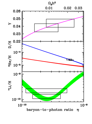
Shown in fig. 18 are the light element predictions with outlined boxes showing the observational constraints and the $\eta$ ranges allowed by each. There is no value of baryon density for which any three abundance observations agree well, as seen quantitatively in tab. 3. Treating all observations equally, we can only reliably constrain the baryon-to-photon ratio to lie between $1\mathrel{\mathchoice{\lower 3.6pt\vbox{\halign{$\mathsurround=0pt\displaystyle\hfil#\hfil$\cr<\crcr\sim\crcr}}}{\lower 3.6pt\vbox{\halign{$\mathsurround=0pt\textstyle\hfil#\hfil$\cr<\crcr\sim\crcr}}}{\lower 3.6pt\vbox{\halign{$\mathsurround=0pt\scriptstyle\hfil#\hfil$\cr<\crcr\sim\crcr}}}{\lower 3.6pt\vbox{\halign{$\mathsurround=0pt\scriptscriptstyle\hfil#\hfil$\cr<\crcr\sim\crcr}}}}10^{10}\eta\mathrel{\mathchoice{\lower 3.6pt\vbox{\halign{$\mathsurround=0pt\displaystyle\hfil#\hfil$\cr<\crcr\sim\crcr}}}{\lower 3.6pt\vbox{\halign{$\mathsurround=0pt\textstyle\hfil#\hfil$\cr<\crcr\sim\crcr}}}{\lower 3.6pt\vbox{\halign{$\mathsurround=0pt\scriptstyle\hfil#\hfil$\cr<\crcr\sim\crcr}}}{\lower 3.6pt\vbox{\halign{$\mathsurround=0pt\scriptscriptstyle\hfil#\hfil$\cr<\crcr\sim\crcr}}}}7$. There is only marginal agreement at the 95% confidence level. This marginal concordance is also evaluated in previous works cfo1 ; cfo2 with the use of theory and observationally based likelihoods ostys ; ot97 ; ot99 ; lisi . If we limit ourselves to D only constraints we find that $10^{10}\eta=6.28^{+0.34}_{-0.35}$ and $5.92^{+0.55}_{-0.58}$, for the multiple absorption and world averages respectively.

Table 3: This table lists the baryon density constraints placed by various light element observations using this works theory predictions. For comparison, the WMAP team’s result for the baryon density is also shown. The numbers cited are the mostly likely values and their respective 68% central confidence limits. Since the bonifacio ${}^{7}{\rm Li}$ constraint lies above the “dip” in the theory prediction, it has two distinct predictions for the baryon density, a low baryon density constraint $I$ and a high baryon density constraint $II$.

Observations	$\eta_{10}\equiv 10^{10}\eta$	$\Omega_{\rm B}h^{2}$
D/H = $(2.49^{+0.20}_{-0.18})\times 10^{-5}$ omeara ; kirkman	$6.28^{+0.34}_{-0.35}$	$0.0229\pm 0.0013$
D/H = $(2.78^{+0.44}_{-0.38})\times 10^{-5}$ burlestytler ; omeara ; kirkman ; pettini	$5.92^{+0.55}_{-0.58}$	$0.0216^{+0.0020}_{-0.0021}$
$Y_{p}=0.238\pm 0.002\pm 0.005$ fieldsolive	$2.39^{+1.75}_{-0.87}$	$0.0087^{+0.0064}_{-0.0031}$
$Y_{p}=0.244\pm 0.002\pm 0.005$ izotovthuan	$3.95^{+3.54}_{-1.64}$	$0.0144^{+0.0129}_{-0.0060}$
${}^{7}{\rm Li}$/H = $(1.23\pm 0.03^{+0.34}_{-0.16})\times 10^{-10}$ryan	$3.19^{+0.41}_{-1.23}$	$0.0116^{+0.0015}_{-0.0044}$
${}^{7}{\rm Li}$/H = $(2.19^{+0.46}_{-0.38})\times 10^{-10}$bonifacio	${}^{I}1.49^{+0.25}_{-0.22}$	$0.0055^{+0.0009}_{-0.0008}$
“     “	${}^{II}4.41^{+0.57}_{-0.51}$	$0.0161^{+0.0021}_{-0.0019}$
WMAP (2003) wmap	$6.14\pm 0.25$	$0.0224\pm 0.0009$

This tension could either be pointing out unknown systematics in the abundance observations, or be telling us that there is new physics to be learnt. We address both of these in the following sections. An independent measure of the baryon density will eliminate it as a free parameter for BBN. This independent determination will act as a tie-breaker among light element observations and lead the way to understanding this tension, whether the disagreement results from underlying systematics or new physics.

IV.2 Observational Concordance

As mentioned at the beginning of the work, the CMB anisotropies detail information about the shape and content of our universe. With the first data release of the WMAP team wmap , several cosmological parameters have been measured to unprecedented accuracy, including the baryon density, which is measured to be,

$$\Omega_{\rm B}h^{2}=0.0224\pm 0.0009.$$ (53)

This corresponds with a baryon-to-photon ratio of $\eta=(6.14\pm 0.25)\times 10^{-10}$. This is a 4% measurement, which makes it a sharper baryon probe than any light element currently is. Since we no longer are required to use the light element abundances to tell us the baryon content of the universe, the analysis completely changes. Now we can predict the light element abundances, with this baryon density and compare those predictions with the light element observations. With WMAP’s baryon density we get:

$$Y_{p} = 0.2485\pm 0.0005$$ (54)

$${\rm D/H} = \left(2.55^{+0.21}_{-0.20}\right)\times 10^{-5}$$ (55)

$$\mbox{${}^{3}{\rm He}$}/{\rm H} = \left(10.12^{+0.67}_{-0.66}\right)\times 10^{-6}$$ (56)

$$\mbox{${}^{7}{\rm Li}$}/{\rm H} = \left(4.26^{+0.91}_{-0.86}\right)\times 10^{-10}$$ (57)

for the light element predictions with our new nuclear reaction network. Figure 19 shows the predictions and compares them directly with observations.

Figure 19: Primordial light element abundances as predicted by BBN and WMAP (dark shaded regions). Different observational assessments of primordial abundances are plotted as follows: (a) the light shaded region shows ${\rm D/H}=(2.78^{+0.44}_{-0.38})\times 10^{-5}$burlestytler ; omeara ; kirkman ; pettini , while the dashed curve shows ${\rm D/H}=(2.49^{+0.20}_{-0.18})\times 10^{-5}$omeara ; kirkman ; (b) no observations plotted; see text (c) the light shaded region shows $Y_{p}=0.238\pm 0.002\pm 0.005$ fieldsolive , while the dashed curve shows $Y_{p}=0.244\pm 0.002\pm 0.005$ izotovthuan ; (d) the light shaded region shows $\mbox{${}^{7}{\rm Li}$}/{\rm H}=(1.23^{+0.34}_{-0.16})\times 10^{-10}$ ryan , while the dashed curve shows $\mbox{${}^{7}{\rm Li}$}/{\rm H}=(2.19^{+0.46}_{-0.38})\times 10^{-10}$ bonifacio .

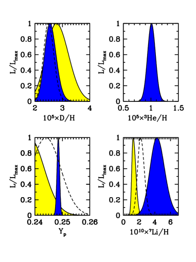
In order to quantify the level of concordance, we define an effective $\chi^{2}$.

$$\chi^{2}_{eff}=\frac{(A_{obs}-A_{wmap})^{2}}{\sigma_{obs}^{2}+\sigma_{wmap}^{2}},$$ (58)

where $A_{obs}$ and $A_{wmap}$ are the most likely values of the light element abundances for the adopted observations and that predicted with the WMAP baryon density. $\sigma_{obs}$ and $\sigma_{wmap}$ are the corresponding 68% confidence errors. The $\chi^{2}$ values are shown in tab. 4.

Table 4: This table lists the effective $\chi^{2}$’s for each observational constraint of the light element abundances, given the WMAP baryon density and this compilation’s BBN theory. A $\chi^{2}_{eff}$ value smaller than unity means concordance, while a value large than unity shows discordance. The magnitude of discordance is measured by $\sqrt{\chi^{2}_{eff}}$, a measure of how many “$\sigma$” of discordance exists.

Observations	$\chi^{2}_{eff}$	$\sqrt{\chi^{2}_{eff}}$
D/H = $(2.49^{+0.20}_{-0.18})\times 10^{-5}$ omeara ; kirkman	0.045	0.212
D/H = $(2.78^{+0.44}_{-0.38})\times 10^{-5}$ burlestytler ; omeara ; kirkman ; pettini	0.281	0.530
$Y_{p}=0.238\pm 0.002\pm 0.005$ fieldsolive	3.77	1.94
$Y_{p}=0.244\pm 0.002\pm 0.005$ izotovthuan	0.692	0.832
$Y_{p}=0.238\pm 0.002$ fieldsolive	25.9	5.09
$Y_{p}=0.244\pm 0.002$ izotovthuan	4.77	2.18
${}^{7}{\rm Li}$/H = $(1.23\pm 0.03^{+0.34}_{-0.16})\times 10^{-10}$ryan	10.72	3.27
${}^{7}{\rm Li}$/H = $(2.19^{+0.46}_{-0.38})\times 10^{-10}$bonifacio	4.50	2.12

As one can see, the two adopted observational values of deuterium agree with the BBN+WMAP prediction, both having $\chi^{2}_{eff}$’s smaller than unity. It is unclear if the slightly worse $\chi^{2}$ of the world average is due to unknown systematics or just poor statistics. Hopefully, with future automated searches, many more of these special absorption systems can be found. It is interesting to note that the WMAP baryon density contributes significantly to the uncertainty in the predicted D abundance. Future CMB experiments will reduce this uncertainty, at which time the BBN nuclear uncertainties will totally dominate the theory predictions. Thus motivating renewed efforts for new cross section measurements.

The Izotov and Thuan value, $Y_{p}=0.244$ izotovthuan value agrees with theory predictions only if the systematic errors are taken into account as discussed earlier. If they are ignored, this number shows discordance at more than the 2-$\sigma$ level. The Fields and Olive value, $Y_{p}=0.238$ fieldsolive shows discordance at the 2-$\sigma$ level with systematic uncertainties. If they are ignored here, the discordance becomes a 5-$\sigma$ deviation. It is clear that a more detailed study of these systematics, including the effects of underlying stellar absorption and varying treatments of emission lines, is needed OSk . One may also consider the new evaluation by Izotov and Thuan newIT , finding $Y_{p}=0.2421\pm 0.0021$, a nearly 3-$\sigma$ deviation with this compilation’s CMB+BBN predictions. We believe a proper accounting of the systematic errors will alleviate this discordance.

The CMB itself, is also sensitive to the value of $Y_{p}$. First attempts at constraining $Y_{p}$ have been performed by Trotta and Hansen trothan and by Huey, Cyburt and Wandelt hcw . Future parameter studies, should include $Y_{p}$ as a free parameter, rather than adopting the canonical value of 0.24. The CMB constraint offers an independent determination, free of the systematics plaquing the determination from extra-galactic HII regions. It also is a direct probe of $Y_{p}$, so no extrapolations to zero metallicity are needed for the determination, just high precision CMB anisotropy data. With this data, we can use the CMB-determined $Y_{p}$ to quantify the level of observational systematics discussed above. By combining BBN predictions with CMB observations, we can also learn about stellar evolution bono ; cassisi . One should also be mindful of the baryon density dependence on $Y_{p}$ given in eqn. 1, especially when combining BBN and CMB results.

The WMAP+BBN prediction for ${}^{7}{\rm Li}$ disagrees with both observationally-based primordial ${}^{7}{\rm Li}$ abundances, with the Ryan et al. ryan and Bonifacio et al. bonifacio numbers showing discordance at the 3 and 2-$\sigma$ level. As already mentioned, the difference between these two sets of observations is a measure of the systematic error due to the different methods used. This is not large enough to account for all of the discrepency between the observation-based and predicted values. An often discussed possibility is the depletion of atmospheric ${}^{7}{\rm Li}$. This possibility faces the strong constraint that the observed lithium abundances show extremely little dispersion, making it unlikely that stellar processes which depend on the temperature, mass, and rotation velocity of the star all destroy ${}^{7}{\rm Li}$ by the same amount. Uniform depletion factors of order 0.2 dex (a factor of 1.6) have been discussed dep . It is clear that either (or both) the base-line abundances of ${}^{7}{\rm Li}$ have been poorly derived or stellar depletion is far more important than previously thought. Of course, it is possible that if systematic errors can be ruled out, a persistent discrepancy in ${}^{7}{\rm Li}$ could point to new physics.

IV.3 Implications for non-standard BBN

With the goal of maintaining concordance with observations, we examine how sharply we can deviate from the standard model. Often the effect of new physics can be parameterized in terms of additional relativistic degrees of freedom during the epoch of primordial nucleosynthesis, usually expressed in terms of the effective number of neutrino species, $N_{\nu,eff}$. Traditionally, D or ${}^{7}{\rm Li}$ observations were used to fix the baryon density and the ${}^{4}{\rm He}$ mass fraction was used to fix $N_{\nu,eff}$. These limits are thoroughly described elsewhere cfo2 ; ssg ; flsv ; dolgov . Moreover, as we have noted, the observed ${}^{4}{\rm He}$ appears lower than the WMAP+BBN value. This discrepancy is likely due to systematic errors, but could point to new physics. Until this situation is better understood, caution is in order. Fortunately, in the post-WMAP era, we can now use the CMB-determined baryon density (eqn. 53), to remove it as a free parameter from BBN theory and use any or all abundance observations to constrain $N_{\nu,eff}$ cfo2 ; cfo3 ; cimm ; hannestad ; barger . In particular, we have computed the likelihood distributions for $N_{\nu,eff}$ using the WMAP $\eta$ and several of the light element observations.

Figure 20: The light element predictions plotted against the baryon-to-photon ratio for different values for $N_{\nu,eff}$. The light shaded region corresponds with $N_{\nu,eff}=2.0$, the medium shaded with $N_{\nu,eff}=4.0$ and the dark shaded with $N_{\nu,eff}=3.0$.

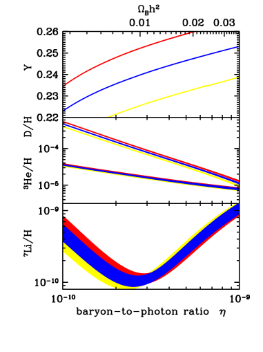
To first gauge what elements are sensitive to $N_{\nu,eff}$, we have plotted the primordial abundance predictions for the standard case, $N_{\nu,eff}=3$, and two non-standard cases, $N_{\nu,eff}=2,4$ in fig. 20. As readily apparent, ${}^{4}{\rm He}$ is the most sensitive element. If we understood the underlying systematics with the ${}^{4}{\rm He}$ observations better, this would be the ideal choice for picking an observation to make the constraint. However, since we are unsure about ${}^{4}{\rm He}$, we must move to another observation. We see that D is the next most sensitive, and most notably, with this new compilation, the differences between the 3 $N_{\nu,eff}$’s are clearly resolvable. With current theory and observation uncertainties, ${}^{7}{\rm Li}$ is not very sensitive to the relativistic degrees of freedom at the high baryon densities that the CMB prefers, thus making it not suitable for this analysis.

To gauge the kinds of constraints we can place, we calculate both ${}^{4}{\rm He}$ and D constraints seen in tab. 5. The ${}^{4}{\rm He}$ observations that appear systematically low in the standard case, $N_{\nu,eff}=3$, pull down the most likely value of $N_{\nu,eff}$ to lie between 2 and 3 depending on which abundance we favor. With our concerns of systematics in ${}^{4}{\rm He}$ observations, we do not put much weight in the ${}^{4}{\rm He}$-based constraints, but we do note that the Izotov and Thuan izotovthuan $Y_{p}$ determination is in fair agreement with the Standard Model of Particle phyics value of $N_{\nu,eff}=3.0$, as long as systematic errors are taken into account. However, the $N_{\nu,eff}=3.0$ D prediction is in accord with the CMB baryon density, thus yielding less pull away from $N_{\nu,eff}=3.0$ in the non-standard model. It is very interesting that each observation’s most likely $N_{\nu,eff}$ lie on opposite sides of the standard BBN value of 3. Using the multiple absorption line system average omeara ; kirkman , we find $N_{\nu,eff}=2.78^{+0.87}_{-0.76}$. With the world average, we find $N_{\nu,eff}=3.65^{+1.46}_{-1.30}$. Even though D’s dependence on $N_{\nu,eff}$ is smaller than its dependence on the baryon density, a sufficiently accurate measurement (e.g. WMAP) of $\eta$, will help make D a more accurate probe. Thus demanding both improved nuclear data and more D observations.

Table 5: This table lists the $N_{\nu,eff}$ constraints placed by various light element observations using this works theory predictions and the WMAP team’s baryon density, $\Omega_{\rm B}h^{2}=0.0224\pm 0.0009$ wmap . The numbers cited are the mostly likely values and their respective 68% central confidence limits.

Observations	$N_{\nu,eff}$
D/H = $(2.49^{+0.20}_{-0.18})\times 10^{-5}$ omeara ; kirkman	$2.78^{+0.87}_{-0.76}$
D/H = $(2.78^{+0.44}_{-0.38})\times 10^{-5}$ burlestytler ; omeara ; kirkman ; pettini	$3.65^{+1.46}_{-1.30}$
$Y_{p}=0.238\pm 0.002\pm 0.005$ fieldsolive	$2.26^{+0.37}_{-0.36}$
$Y_{p}=0.244\pm 0.002\pm 0.005$ izotovthuan	$2.67^{+0.40}_{-0.38}$

V Conclusions

Primordial nucleosynthesis has entered a new era. With the precision observations of WMAP, the CMB has become the premier cosmic baryometer. The independent BBN and CMB predictions for $\eta$ are in good agreement (particularly when D is used in BBN), indicating that cosmology has passed a fundamental test. Moreover, this agreement allows us to use BBN in a new way, as the CMB removes $\eta$ as a free parameter. One can then adopt the standard BBN predictions, and use $\eta_{\rm CMB}$ to infer primordial abundances; by comparing these to light element abundances in different settings, one gains new insight into the astrophysics of stars, HII regions, cosmic rays, and chemical evolution, to name a few examples. Alternately, WMAP transforms BBN into a sharper probe of new physics in the early universe; with $\eta_{\rm CMB}$ fixed, all of the light elements constrain non-standard nucleosynthesis, with $N_{\rm\nu,eff}$ being one example.

As BBN assumes a new role, much work remains to be done. To leverage the power of the WMAP precision requires the highest possible precision in light element observations. Further improvements in the primordial D abundance can open the door to D as a powerful probe of early universe physics. Improved ${}^{3}{\rm He}$ observations can offer new insight into stellar and chemical evolution in the Galaxy. And perhaps most pressing, the WMAP prediction for primordial ${}^{4}{\rm He}$ and particularly ${}^{7}{\rm Li}$ are higher than the current observed abundances; it remains to be resolved what systematic effects (or new physics!) has led to this discrepancy.

This work has always been motivated by the idea of precision cosmology. We have laid out a rigorous procedure for determining best fit parameters and their uncertainties. We have explicitly taken into account the correlations among data points and their normalization errors. We found it necessary to define two systematic uncertainties, one is a calculation of the inherent normalization of the data. The second is a measure of how well different data sets agree with each other. This work generally agrees with previous studies, except in some special cases as discussed.

Using these updated nuclear inputs, we compute the new BBN abundance predictions, and quantitatively examine their concordance with observations. BBN theory uncertainties are dominated by the following reactions: $d(d,n)\mbox{${}^{3}{\rm He}$}$, $d(d,p)t$, $d(p,\gamma)\mbox{${}^{3}{\rm He}$}$, $\mbox{${}^{3}{\rm He}$}(\alpha,\gamma)\mbox{${}^{7}{\rm Be}$}$ and $\mbox{${}^{3}{\rm He}$}(d,p)\mbox{${}^{4}{\rm He}$}$. Reducing BBN’s uncertainties will allow stronger statements about concordance. Depending on what deuterium observations are adopted, one gets the following constraints on the baryon density: $\Omega_{\rm B}h^{2}=0.0229\pm 0.0013$ or $\Omega_{\rm B}h^{2}=0.0216^{+0.0020}_{-0.0021}$ at 68% confidence. If we instead adopt the WMAP baryon density, we find the following constraints on the effective number of neutrinios during BBN: $N_{\nu,eff}=2.78^{+0.87}_{-0.76}$ or $N_{\nu,eff}=3.65^{+1.46}_{-1.30}$ at 68% confidence. Concerns over systematics in helium and lithium observations limit the confidence of the constraints derived from this data. Further exploration of these systematics, given new observational techniques and more detailed models, will be most beneficial in understanding and ultimately reducing their effects. Deuterium suffers from a small sample size; a larger sample size will not only improve statistics but also allow the examination of possible systematics. With new nuclear cross section data, light element abundance observations and the ever increasing resolution of the CMB anisotropy, tighter constraints can be placed on nuclear and particle astrophysics.

In closing, it is impressive that our now-exquisite understanding of the universe at $z\sim 1000$ also confirms our understanding of the universe at $z\sim 10^{10}$. This agreement lends great confidence in the soundness of the hot big bang cosmology, and impels our search deeper into the early universe.

Appendix A Cross Section Fits

A.1 $d(p,\gamma)\mbox{${}^{3}{\rm He}$}$

$S(E)=0.2268(1+22.05E+30.77E^{2}-9.919E^{3}){\rm\ eV\ b}$,

A.2 $d(d,n)\mbox{${}^{3}{\rm He}$}$

$S(E)=0.05067(1+7.534E-4.225E^{2}+1.508E^{3}-0.2041E^{4}){\rm\ MeV\ b}$

A.3 $d(d,p)t$

$S(E)=0.05115(1+4.685E-1.021E^{2}){\rm\ MeV\ b}$

A.4 $\mbox{${}^{3}{\rm He}$}(n,p)t$

$R(E)=6.846\times 10^{8}(1.-0.464743311577E-01E^{1/2}-0.206566636058E+02E\\ +145.303829979E^{3/2}-517.845305322E^{2}+1061.59032882E^{5/2}-1232.39931680E^{3}\\ +748.452414743E^{7/2}-184.417975062E^{4}){\rm\ cm^{3}\ g^{-1}s^{-1}}$

A.5 $t(d,n)\mbox{${}^{4}{\rm He}$}$

$S(E)=24.19(1+3.453E-40.16E^{2}+285.6E^{3}-596.4E^{4}+407.1E^{5})/(1+\left(\frac{E-E_{R}}{\Gamma_{R}/2}\right)^{2}){\rm\ MeV\ b},$
where $E_{R}=0.0482$ MeV and $\Gamma_{R}=0.0806$ MeV.

A.6 $\mbox{${}^{3}{\rm He}$}(d,p)\mbox{${}^{4}{\rm He}$}$

$S(E)=18.52(1-4.697E+39.53E^{2}-109.6E^{3}+130.7E^{4}-54.83E^{5})/(1+\left(\frac{E-E_{R}}{\Gamma_{R}/2}\right)^{2}){\rm\ MeV\ b},$
where $E_{R}=0.183$ MeV and $\Gamma_{R}=0.256$ MeV.

A.7 $\mbox{${}^{3}{\rm He}$}(\alpha,\gamma)\mbox{${}^{7}{\rm Be}$}$

$S(E)=0.3861(1+0.8195E-2.194E^{2}+1.419E^{3}-0.2780E^{4}){\rm\ keV\ b}$

A.8 $t(\alpha,\gamma)\mbox{${}^{7}{\rm Li}$}$

$S(E)=0.08656(1+0.6442E-7.597E^{2}+12.16E^{3}-5.336E^{4}){\rm\ keV\ b}$

A.9 $\mbox{${}^{7}{\rm Be}$}(n,p)\mbox{${}^{7}{\rm Li}$}$

$R(E)=4.7893\times 10^{9}(1-4.12682044152E^{1/2}+3.10200988738E\\ +15.8164551655E^{3/2}-45.5822669937E^{2}+54.7133921087E^{5/2}-34.7483784037E^{3}\\ +11.3599443403E^{7/2}-1.49669812741E^{4})+1.0553\times 10^{9}/(1.+((E-E_{R,1})/(0.5\Gamma_{R,1}))^{2})\\ +2.0364\times 10^{9}/(1.+((E-E_{R,2})/(0.5\Gamma_{R,2}))^{2}){\rm\ cm^{3}\ g^{-1}s^{-1}}$
where $E_{R,1}=0.32$ MeV, $\Gamma_{R,1}=0.20$ MeV, $E_{R,2}=2.7$ MeV, and $\Gamma_{R,2}=1.9$ MeV.

A.10 $\mbox{${}^{7}{\rm Li}$}(p,\alpha)\mbox{${}^{4}{\rm He}$}$

$S(E)=0.06068(1+3.174E-7.586E^{2}+8.539E^{3}-3.216E^{4}){\rm\ MeV\ b}$

Appendix B Thermal Rates

In adopting these rates, it is a good idea to assume the rate constant at temperatures above which these fits are no longer valid (see table 2). This prevents the artificial divergence of the abundances.

B.1 $p(n,\gamma)d$

$N_{A}\langle\sigma v\rangle$ = 4.40654e4*(1.+.0457518*t912-2.47101*t9+4.17185*t932
-3.44553*t9*t9+1.72766*t9*t932-.546196*t9**3
+.106066*t912*t9**3-.0115306*t9**4+.536436e-3*t912*t9**4)

B.2 $d(p,\gamma)\mbox{${}^{3}{\rm He}$}$

$N_{A}\langle\sigma v\rangle$ = 7.30909e+3*t9m23*ex(-3.7209/t913)
*(1.-10.3497*t913+63.4315*t923-209.780*t9
+432.557*t943-571.937*t953+497.303*t9*t9
-284.936*t943*t9+106.863*t953*t9-25.7496*t9**3
+3.81387*t913*t9**3-.313823*t923*t9**3+.0108908*t9**4)

B.3 $d(d,n)\mbox{${}^{3}{\rm He}$}$

$N_{A}\langle\sigma v\rangle$ = 1.00749e+9*t9m23*ex(-4.2586/t913)
*(1. -9.59015*t913+65.2448*t923-247.756*t9
+596.231*t943-941.064*t953+980.076*t9*t9
-643.032*t9*t943+211.982*t9*t953+29.0491*t9**3
-66.1847*t913*t9**3+31.6452*t923*t9**3-7.15147*t9**4
+.372749*t913*t9**4+.208645*t923*t9**4-.0545129*t9**5
+.00536216*t913*t9**5-.000157984*t923*t9**5
-.457514e-5*t9**6+2.123592e-9*t913*t9**6)

B.4 $d(d,p)t$

$N_{A}\langle\sigma v\rangle$ = 3.91889e+8*t9m23*ex(-4.2586/t913)
*(1.+.309233*t913-.337260*t923+2.51922*t9
-2.79097*t943+2.16082*t953-.976181*t9*t9
+.210883*t943*t9-.0169027*t953*t9+7.845538e-6*t9**3)

B.5 $\mbox{${}^{3}{\rm He}$}(n,p)t$

$N_{A}\langle\sigma v\rangle$ = 6.84713e+8*(1.-.0171094*t912-2.66179*t9+8.27463*t932
-14.3898*t9*t9+15.6385*t932*t9-10.3337*t9**3
+3.80177*t912*t9**3-.599790*t9**4-.0139213*t912*t9**4
+.0140311*t9**5-.00106709*t912*t9**5+1.06709e-6*t9**6)

B.6 $t(d,n)\mbox{${}^{4}{\rm He}$}$

$N_{A}\langle\sigma v\rangle$ = 1.78988e12*t9m23*ex(-4.5245/t913)
/(1. + ((0.129964*t923-0.0482)/(0.5*0.0806))**2)
*(1.-14.3137899*t913+92.4325675*t923
-314.645738*t9+641.100355*t943-844.106855*t953
+752.418564*t9*t9-465.820564*t943*t9
+202.276143*t953*t9-61.3172473*t9**3
+12.6913874*t913*t9**3-1.707344*t923*t9**3
+.134399048*t9**4-.00469341945*t913*t9**4)

B.7 $\mbox{${}^{3}{\rm He}$}(d,p)\mbox{${}^{4}{\rm He}$}$

$N_{A}\langle\sigma v\rangle$ = 5.67897e12*t9m23*ex(-7.1840/t913)
/(1. + ((0.206357*t923-0.183)/(0.5*0.256))**2)
*(1.-8.59410908*t913+31.1979775*t923
-61.2218616*t9+72.0331037*t943-52.8696341*t953
+23.7371543*t9**2-5.4569107*t943*t9-.226478266*t953*t9
+.583380161*t9**3-.190978484*t913*t9**3
+.031949394*t923*t9**3-.00284146599*t9**4
+.106749198e-3*t913*t9**4)

B.8 $\mbox{${}^{3}{\rm He}$}(\alpha,\gamma)\mbox{${}^{7}{\rm Be}$}$

$N_{A}\langle\sigma v\rangle$ = 3.94207e+6*t9m23*ex(-12.8274/t913)
*(1. + .185267*t913 - .837432*t923
+7.23019*t9 - 26.1976*t943 +41.6914*t953
+19.4465*t9*t9-215.248*t9*t943+422.548*t9*t953
-412.866*t9**3+176.691*t913*t9**3+45.8891*t923*t9**3
-100.644*t9**4+54.8984*t913*t9**4-14.1903*t923*t9**4
+1.48464*t9**5)

B.9 $t(\alpha,\gamma)\mbox{${}^{7}{\rm Li}$}$

$N_{A}\langle\sigma v\rangle$ = 4.65494351e+6*t9m23*ex(-8.0808/t913)
*(1. - 12.3956341*t913 + 76.2717899*t923
-250.678479*t9+446.413119*t943 -289.008201*t953
-474.786707*t9*t9 +1346.42142*t9*t943 -1503.09444*t9*t953
+923.138882*t9**3-306.14089*t913*t9**3+42.9886919*t923*t9**3)

B.10 $\mbox{${}^{7}{\rm Be}$}(n,p)\mbox{${}^{7}{\rm Li}$}$

$N_{A}\langle\sigma v\rangle$ = 5.17900e9*(1.-1.44587*t912+1.12925*t9-.493526*t932
+.126269*t9*t9-.0194265*t932*t9+.00177188*t9**3
-.883411e-4*t912*t9**3+.185551e-5*t9**4)
+4.2994e9*t9m32*ex(-3.713442/t9)
+1.36949e11*t9m32*ex(-31.332167/t9)

B.11 $\mbox{${}^{7}{\rm Li}$}(p,\alpha)\mbox{${}^{4}{\rm He}$}$

$N_{A}\langle\sigma v\rangle$ = 9.19322e8*t9m23*ex(-8.4730/t913)
*(1. - 2.26222*t913 + 11.3224*t923
- 27.3071*t9 + 41.1901*t943 - 37.4242*t953
+ 18.3941*t9*t9 -3.72281*t9*t943 +2.58125e-2*t953*t9)

References

- (1) Hubble, E. 1929 Proceedings of the National Academy of Science 15, 168
- (2) Gamow, G. 1946 Phys. Rev. 70, 572
- (3) Alpher, R.A., Bethe, H. & Gamow, G. 1948 Phys. Rev. 73, 803
- (4) Hayashi, C. 1950 Prog. Theor. Phys., 5, 224
- (5) Alpher, R.A., Follin, J.W. & Herman, R.C. 1953 Phys. Rev. 92, 1347
- (6) Alpher, R.A. & Herman, R.C. 1948 Phys. Rev. 74, 1737
- (7) Alpher, R.A. & Herman, R.C. 1949 Phys. Rev. 75, 1089
- (8) Penzias, A.A. & Wilson, R.W. 1965 ApJ 142, 419
- (9) Peebles, P.J.E. 1966 Phys. Rev. Lett. 16, 410
- (10) Wagoner, R.V., Fowler, W.A., & Hoyle,F. 1967 ApJ 148, 3
- (11) Mather, J.C. et al. 1990 ApJ 354, L37 (COBE)
-
(12)
Balbi, A. et al. 2000 ApJ 545 L1 [astro-ph/0005124] (MAXIMA)
Balbi, A. et al. 2001 ApJ 558 L145 -
(13)
Ruhl, J.E. et al. 2003 ApJ 599, 786 [astro-ph/0212229] (BOOMERANG)
Netterfields, C.B. et al. 2002 ApJ 571, 604 [astro-ph/0104460] - (14) Pryke., C. et al. 2002 ApJ 568, 46 [astro-ph/0104490] (DASI)
- (15) Sievers, J.L. et al. 2003 ApJ 591, 599 [astro-ph/0205387] (CBI)
- (16) Kuo, C.L. et al. 2004 ApJ 600, 32 [astro-ph/0212289] (ACBAR)
(17)
Bennett, C.L. et al. 2003 ApJS 148, 1 [astro-ph/0302207] (WMAP)
Spergel, D.N. et al. 2003 ApJS 148, 175 [astro-ph/0302209] - (18) Schramm, D.N. & Wagoner, R.V. 1979 Ann. Rev. Nucl. & Part. Sci., 27, 37
- (19) Yang, J. et al. 1984 ApJ, 281, 493
- (20) Boesgaard, A.M. & Steigman, G. 1985 Ann. Rev. Astron. & Astoph., 23, 319
- (21) Kolb, E.W. & Turner, M.S. 1990 “The Early Universe” Reading, MA: Addison-Wesley
- (22) Walker, T.P. et al. 1991 ApJ 376, 51
- (23) Sarkar, S. 1996 Rep. Prog. Phys. 59, 1493
- (24) Olive, K.A., Steigman, G. & Walker, T.P. 2000 Phys. Rep. 333, 389
- (25) Tytler, D. et al. 2000 Phys. Rept., 333, 409
- (26) Hagiwara, K. et al 2002 Phys. Rev. D 66, 010001
- (27) White, M., Scott, D. & Silk, J. 1994 Ann. Rev. Astron. & Astoph., 32, 319
- (28) Tegmark, M. 1996 Dark Matter in the Universe, Italian Physical Society, Proc. Internat. School of Physics Course CXXXII, Varenna on Lake Como, Villa Monastero. Oxford, GB: IOS Press, 379. [astro-ph/9511148]
- (29) Van der Veen, J. et al. 1998 The Physics Teacher, 36, 529
- (30) Kamionkowski, M. & Kosowsky, A. 1999 Ann. Rev. Nucl. & Part. Sci., 49, 77
- (31) Hu, W. & Dodelson, S. 2002 Ann. Rev. Astron. & Astoph., 40, 171
- (32) Wang, X. et al. 2003 Phys. Rev. D68, 123001 [astro-ph/0212417]
- (33) Krauss, L.M. & Romanelli, P. 1990 ApJ 358, 47
- (34) Smith, M.S., Kawano, L.H. & Malaney, R.A. 1993 ApJS 85, 219
- (35) Krauss, L.M. & Kernan, P. 1995 Phys. Lett. B347, 347
- (36) Hata, N. et al. 1996 ApJ 458, 637
- (37) Fiorentini, G. et al. 1998 Phys. Rev. D58, 063506
- (38) Nollett, K.M. & Burles, S. 2000 Phys. Rev. D61, 123505
- (39) Cyburt, R.H., Fields, B.D. & Olive, K.A. 2001 New Astron. 6, 215 [astro-ph/0102179]
- (40) Coc, A. et al. 2002 Phys. Rev. D65, 043510
- (41) Steigman, G., S. Schramm, D.N. & Gunn, J. 1977 Phys. Lett. B 66, 202
- (42) Dolgov, A.D. 2002 Nuovo Cimento B Serie, 117, 1081
- (43) Jungman, G. et al. 1995 Phys. Rev. D54, 1332
- (44) Schramm, D.N. & Turner, M.S. 1998 Rev. Mod. Phys. 70, 303 [astro-ph/9706069]
- (45) Burles, S., Nollett, K.M. & Turner, M.S. 2001 Phys. Rev. D 63, 063512 [astro-ph/0008495]
- (46) Cyburt, R.H., Fields, B.D. & Olive, K.A. 2002 Astropart. Phys. 17, 87 [astro-ph/0105397]
- (47) Cyburt, R.H., Fields, B.D. & Olive, K.A. 2003 Phys. Lett. B 567, 227 [astro-ph/0302431]
- (48) D’Agostini, G. 1994 Nucl. Instrum. Meth. A346, 306
- (49) Clayton, D.D. 1983 Univerity of Chicago Press, Chicago, “Principles of Stellar Evolution and Nucleosynthesis”
- (50) Rolfs, C.E. & Rodney, W.S. 1988 University of Chicago Press, Chicago, “Cauldrons in the Cosmos: Nuclear Astrophysics”
- (51) Fowler, W.A., Caughlan, G.R. & Zimmerman, B.A. 1967 Annl. Rev. Astron. and Astrph. 5, 525
- (52) Fowler, W.A., Caughlan, G.R. & Zimmerman, B.A. 1975 Annl. Rev. Astron. and Astrph. 13, 69
- (53) Caughlan, G.R. & Fowler, W.A. 1988 A. Data and Nucl. Data Tabl. 40, 283
- (54) Angulo, C. et al. 1999 Nucl. Phys. A656, 3
(55)
Nuclear Data Centers Network, EXFOR Systems Manual:
Nuclear Reaction Data Exchange Format, Report BNL-NCS-63330 (1996),
compiled and edited by V. McLane, National Nuclear Data Center, Brookhaven
National Laboratory, USA; see also the website: http://www.nndc.bnl.gov/nndc/exfor/ - (56) Olive, K.A, Schramm, D.N., Turner, M.S., Yang, J. & Steigman, G. 1981 ApJ 246, 557
- (57) Scherrer, R.J. 2004 accepted in Phys. Rev. D [astro-ph/0310699]
- (58) Hale, G.M. & Johnson, A.S. 2003 17th Intn. Conf. on Few-Body Problems in Physics Proceedings, “Results for n+p capture from an R-matrix analysis of N-N scattering”
- (59) Nagai, Y. et al. 1997 Phys. Rev. C 56, 3173
- (60) Suzuki, T.S. et al. 1995 ApJ 439, L59
- (61) Bailey, G.M. et al. 1970 Canadian J. Phys. 48, 3059
- (62) Griffiths, G.M., Larson, E.A. & Robertson, L.P. 1962 Canadian J. Phys. 40, 402 Griffiths, G.M., Lal, M. & Scarfe, C.D. 1963 Canadian J. Phys. 41, 724
- (63) Ma, L. et al. 1997 Phys. Rev. C 55, 588
- (64) Schmid, G.J. et al. 1996 Nucl. Phys. A 607, 139 Schmid, G.J. et al. 1997 Phys. Rev. C 56, 2565
- (65) Casella, C. et al. 2002 Nucl. Phys. A 706, 203
- (66) Cuoco, A. et al. 2003 [astro-ph/0307213]
- (67) Coc, A. et al. 2003 ApJ 600, 544 [astro-ph/0309480]
- (68) Brown, R.E. & Jarmie, N. 1990 Phys. Rev. C 41, 1391
- (69) Krauss, A. et al. 1987 Nucl. Phys. A 465, 150
- (70) Ganeev, A.S. et al. 1958 Sov. J. At. Energy Suppl. 5, 21
- (71) Arnold, W.R. et al. 1954 Phys. Rev. 93, 483
- (72) McNeill, K.G. & Keyser, G.M. 1951 Phys. Rev. 81, 602
- (73) First Research Group, 1985 Chin. J. Nucl. High En. Phys. 9, 723; original article in Chinese, reference from CSISRS.
- (74) Preston, G., Shaw, P.F. & Young, S.A. 1954 Proc. Roy. Soc. 226, 206
- (75) Jarmie, N., Brown, R.E. & Hardekopf, R.A. 1984 Phys. Rev. C 29, 2031
- (76) Schulte, R.L. et al. 1972 Nucl. Phys. A 192, 609
- (77) Davenport, P.A. et al. 1953 Proc. Roy. Soc. A 216, 66
- (78) Grüebler, W. et al. 1972 Nucl. Phys. A 193, 129
- (79) Brune, C.R. et al. 1999 Phys. Rev. C 60, 015801
- (80) Costello, D.G., Friesenhahn, S.J. & Lopez, W.M. 1970 Nucl. Sci. Eng. 39, 409
- (81) Coon, J.H. 1950 Phys. Rev. 80, 488
- (82) Gibbons, J.H. & Macklin, R.L. 1959 Phys. Rev. 114, 571
- (83) Macklin, R.L. & Gibbons, J.H. 1965 EANDC-50-S, Vol. 1, Paper 13
- (84) Batchelor,R., Aves, R. & Skyrme, T.H.R. 1955 Rev. Sci. Instr. 26, 1037
- (85) Borzakov, S.B. et al. 1982 Sov. J. Nucl. Phys. 35, 3
- (86) Alfimenkov, V.P. et al. 1980 Joint Institute for Nucl. Res. preprint R3-80-394
- (87) Allan, D.L. & Poole, M.J. 1950 Proc. Roy. Soc. A 204, 488
- (88) Argo, H.V. et al. 1952 Phys. Rev. 87, 612
- (89) Bame, S.J., Jr. & Perry, J.E., Jr. 1957 Phys. Rev. 107 1616
- (90) Brown, R.E., Jarmie, N. & Hale, G.M. 1987 Phys. Rev. C 35, 1999
- (91) Conner, J.P., Bonner, T.W. & Smith, J.R. 1952 Phys. Rev. 88, 468
- (92) Davidenko, V.A., Pogrebov, I.S. & Saukov, A.I. 1957 J. Nucl. Eng. 2, 258
- (93) Jarmie, N., Brown, R.E. & Hardekopf, R.A. 1984 Phys. Rev. C 29, 2031
- (94) Bonner, T.W., Conner, J.P. & Lillie, A.B. 1952 Phys. Rev. 88, 473
- (95) Geist, W.H. et al. 1999 Phys. Rev. C 60, 054003
- (96) Kunz, W.E. 1955 Phys. Rev. 97, 456
- (97) Möller, W. & Besenbacher, F. 1980 Nucl. Instr. Meth. 168, 111
- (98) Zhichang, L., Jingang, Y. & Xunliang, D. 1977 Chin. J. Sci. Tech. A. Energy 3, 229
- (99) Homgren, H.D. & Johnston, R.L. 1959 Phys. Rev. 113, 1556
- (100) Parker, P.D. & Kavanagh, R.W. 1963 Phys. Rev. 131, 2578
- (101) Nagatani, K., Dwarakanath, M.R. & Ashery, D. 1969 Nucl. Phys. A 128, 325
- (102) Kräwinkel, H. et al. 1982 Z. Phys. A 304, 307
- (103) Robertson, R.G.H. et al. 1983 Phys. Rev. C 27, 11
- (104) Hilgemeier, M. et al. 1988 Z. Phys. A 329, 243
- (105) Osborne, J.L. et al. 1984 Nucl. Phys. A 419, 115
- (106) Adelberger, E.G. et al. 1998 Rev. Mod. Phys. 70, 1265
- (107) Brune, C.R., Kavanagh, R.W. & Rolfs, C. 1994 Phys. Rev. C 50, 2205
- (108) Burnzyński, S. et al. 1987 Nucl. Phys. A 473, 179
- (109) Griffiths, G.M. et al. 1961 Canadian J. Phys. 39, 1397
- (110) Schroder, U. et al. 1987 Phys. Lett. B 192, 55
- (111) Utsunomiya, H. et al. 1990 Phys. Rev. Lett. 65, 847
- (112) Koehler, P.E. et al. 1988 Phys. Rev. C 37, 917
- (113) Sekharan, K.K. et al 1976 Nucl. Instr. Meth. 133, 253
- (114) Taschek, R. & Hemmendinger, A. 1948 Phys. Rev. 74, 373
- (115) Audi, G. & Wapstra, A.H. 1995 Nucl. Phys. A 595, 409
- (116) US Nuclear Data Program, http://www.nndc.bnl.gov/usndp/
- (117) Engstler, S. et al. 1992 Z. Phys. A 342, 471
- (118) Harmon, J.F. 1989 Nucl. Instr. Meth. B 40/41, 507
- (119) Lee, C.C. 1969 J. Kor. Phys. Soc. 2, 1
- (120) Rolfs, C. & Kavanagh, R.W. 1986 Nucl. Phys. A 455, 179
- (121) Spinka, H., Tombrello, T. & Winkler, H. 1971 Nucl. Phys. A 164, 1
- (122) Shinozuka, T., Tanaka, Y. & Sugiyama, K. 1979 Nucl. Phys. A 326, 47
- (123) Assenbaum, H.J., Langanke, K. & Rolfs, C. 1987 Z. Phys. A 327, 461
- (124) Epstein, R.I., Lattimer, J.M. & Schramm, D.N. 1976 Nature 263, 198
- (125) Burles, S. & Tytler, D. 1998 ApJ 499, 699; ApJ 507, 732
- (126) O’Meara, J.M. et al. 2001 ApJ 552, 718 [astro-ph/0011179]
- (127) Kirkman, D. et al. 2003 ApJS 149, 1 [astro-ph/0302006]
- (128) Pettini, M. & Bowen, D.V. 2001 ApJ 560, 41 [astro-ph/0104474]
- (129) Fields, B.D. et al. 2001 ApJ 563, 653
- (130) Peimbert, M., Peimbert, A. & Ruiz, M.T., 2000 ApJ 542, 688
- (131) Olive, K.A., Steigman, G. & Skillman, E., 1997 ApJ 483, 788
- (132) Fields, B.D. & Olive, K.A. 1998 ApJ 506, 177 [astro-ph/9803297]
(133)
Izotov, Y.I. & Thuan, T.X. 1998 ApJ 500, 188
Izotov, Y.I., Thuan, T.X. & Lipovetsky, V.A. 1997 ApJ 108, 1
Izotov, Y.I., Thuan, T.X. & Lipovetsky, V.A. 1994 ApJ 435, 647 - (134) Olive, K.A. & Skillman, E. 2001 New Astron. 6, 119 [astro-ph/0007081]
- (135) Izotov, Y.I. & Thuan, T.X. 2003 ApJ 602, 200 [astro-ph/0310421]
- (136) Trotta, R. & Hansen, S.H. 2003 Phys. Rev. D69, 023509 [astro-ph/0306588]
- (137) Huey, G., Cyburt, R.H. & Wandelt, B.D. 2004 Phys. Rev. D69, 103503 [astro-ph/0307080]
- (138) Bono, G. et al. 2002 ApJ 568, 463 [astro-ph/0112064]
- (139) Cassisi, S., Salaris, M. & Irwin, A.W. 2003 ApJ 588, 862 [astro-ph/0301378]
- (140) Bania, T.M., Rood, R.T. & Balser, D.S. 2002 Nature 415, 54
- (141) Vangioni-Flam, E., Olive, K.A., Fields, B.D. & Cassé, M. 2003 ApJ 585, 611
- (142) Spite, F. & Spite, M. 1982 Astron. & Astrophys. 115, 357
- (143) Ryan, S.G. et al. 2000 ApJL 530, L57
- (144) Bonifacio, P. et al. 2002 Aston. Astrophys. 390, 91
- (145) Olive, K.A. & Thomas, D. 1997 Astropart. Phys. 7, 27
- (146) Olive, K.A. & Thomas, D. 1999 Astropart. Phys. 11, 403
- (147) Lisi, E., Sarkar, S. & Villante, F.L. 1999 Phys. Rev. D 59, 123520
- (148) Vauclair, S. & Charbonnel, C. 1998 ApJ 502, 372
- (149) Hannestad, S. 2003 Journal of Cosm. and Astro-Part. Phys. 5, 4 [astro-ph/0303076]
- (150) Barger et al. 2003 Phys. Lett. B 566, 8 [hep-ph/0305075]