Decomposition of AGN host galaxy images

Abstract

We describe an algorithm to decompose deep images of Active Galactic Nuclei into host galaxy and nuclear components. Currently supported are three galaxy models: A de-Vaucouleurs spheroidal, an exponential disc, and a two-component disc+bulge model. Key features of the method are: (semi-)analytic representation of a possibly spatially variable point-spread function; full two-dimensional convolution of the model galaxy using gradient-controlled adaptive subpixelling; multiple iteration scheme. The code is computationally efficient and versatile for a wide range of applications. The quantitative performance is measured by analysing simulated imaging data. We also present examples of the application of the method to small test samples of nearby Seyfert 1 galaxies and quasars at redshifts $z<0.35$.

1 Introduction

The properties of black holes in galactic nuclei are probably closely linked to the global properties of the galaxies in which they reside. Fuelling these black holes leads to the AGN and quasar phenomenon; investigating AGN host galaxies for various degrees of AGN activity is therefore a necessary step to understand the physical links, and the role of AGNs in galaxy evolution. Because of the high luminosities of the central region – being effectively a point source in optical and near-infrared wavelengths – which often outshines the entire galaxy, quantitative study of quasar hosts is fraught with technical difficulties. New instrumentation has made this task somewhat more feasible. In particular HST with its high spatial resolution has contributed significantly to the study of quasar hosts both at low redshifts (McLure et al. 1999; McLeod & McLeod 2001) and in the early universe (Kukula et al., 2001; Ridgway et al., 2001; Lehnert et al., 1999). However, ground-based imaging under excellent conditions will remain to be competitive, especially with the new 8–10 m class telescopes (e.g. Falomo, Kotilainen & Treves, 2001) using their large photon-collection area and high resolution.

While the mere detection of QSO hosts often requires no more than elementary and intuitive methods such as azimuthal averaging and PSF subtraction, such procedures have repeatedly been suspected of producing quantitatively biased results (e.g., Abraham, Crawford & McHardy 1992; Ravindranath et al. 2001). Quite certainly, they take insufficient advantage of the full spatial image information content. In recent years, some groups have started to develop two-dimensional model fitting codes addressing these issues, with the goal to simultaneously decompose deep QSO images into nuclear and host components in a more objective and unbiased way (e.g., McLure, Dunlop & Kukula 2000; Wadadekar, Robbason & Kembhavi 1999; Schade, Lilly, Le Fevre, Hammer & Crampton 1996). Ideally, such a method should provide the flexibility to be used with a wide range of ground- and space-based datasets, account for non-ideal detector properties, and require no more than standard computing resources.

In this paper we describe our own approach to tackle this task. We first outline some key features of the algorithm, and then discuss the performance of our method as applied to simulated imaging data. Finally we briefly present two samples of low- and intermediate-redshift QSOs as examples of the method’s usefulness. The method is currently used extensively on various large datasets of QSOs, achieving high data throughput for the modelling which is one of the aims for our code. We shall report in detail on these projects in subsequent papers.

2 The method

2.1 Overview

Optical and near-infrared images of quasars are always compounds of a more or less extended host galaxy (which morphologically may be as simple or as complicated as any ‘normal’ galaxy), plus an embedded point source. Analytic models of such configurations invariably require several approximations and simplifications, which in our approach can be summarised as follows:

• The overall surface brightness distribution of the host galaxy can be described by smooth and azimuthally symmetric profile laws, modified only to allow for a certain degree of ellipticity.

• Host galaxy components and active nucleus (in the following: ‘nucleus’ or ‘AGN’) are concentric.

• The solid angle subtended by a given quasar+host is significantly smaller than the field of view.

• The point-spread function (PSF) is either shift-invariant over the field of view, or else its spatial change can be described by low-order multivariate polynomials.

These assumptions are adequate for the type of distant AGN that we are chiefly interested in, but some will break down for very nearby galaxies with highly resolved structural features; such objects are not our primary targets, and we do not consider their specialities in the following.

The model-fitting process can be split up into several distinct tasks, to be executed subsequently:

1. Construction of a variance frame quantifying individual pixel weights, usually by applying Poisson statistics and standard error propagation to object and background counts. This step includes the creation of an optional mask to exclude foreground stars, companion galaxies, cosmics, etc.

2. Identification of stars in the field to be used as PSF references. As the PSF description is fully analytic, even stars fainter than the quasar can yield useful constraints.

3. Determination of an analytic PSF model for the entire field of view, accounting for spatial variability. An optional empirical lookup table can complement this if required.

4. Establishing initial guess parameters for the AGN+host galaxy model.

5. Computation of the actual multiparameter fit by minimising $\chi^{2}$ iteratively, including multiple restarts to avoid trapping in local minima.

6. Estimation of statistical uncertainties by running the model-fitting code on dedicated simulations mimicking the actual data.

We give details on each of these steps in the following sections.

The software was developed under the ESO-MIDAS environment with all computing expensive tasks coded in C. The code itself has not been developed for general public release, but interested groups may receive a test version on a shared risk basis.

2.2 PSF Modelling

2.2.1 Strategy

Knowledge of the point-spread function (PSF) is important in two aspects of the decomposition. First, it is obviously needed to describe the light distribution of the unresolved AGN itself. Any mismatch here could lead to a misattribution of AGN light to the host galaxy or vice versa. Second, for the typical objects of interest the apparent host galaxy structure will strongly depend on the degree of PSF blurring. This process needs somehow to be inverted in order to determine the corresponding structural parameters. In extreme cases, e.g. when even a marginal detection of a faint high-redshift host would be considered a success, accurate PSF control becomes the most important part of the entire analysis.

As long as the image formation process can be approximated by a shift-invariant linear system, the straightforward and most frequently adopted way of obtaining the PSF is to use the image of a bright star in the field of view. However, even within this approximation using a single star has some non-negligible drawbacks, mainly associated with the problem of rebinning: Unless the PSF is strongly oversampled, shifting an observed stellar image to a different position invariably leads to image degradation and consequently to AGN/PSF mismatch. Ironically, at a given spatial sampling this effect is largest for a very narrow PSF, thus for the best seeing. Furthermore, a single PSF star of sufficient brightness to constrain also the low surface brightness wings of the PSF is not always available, an effect which can render entire images effectively useless. Finally, in a few cases even the only available PSF star could be contaminated by a companion star or galaxy, which would introduce severe artefacts into the analysis.

A simple averaging of stellar images to increase the S/N is often prevented by the fact that several large-field imagers, even modern ones, show spatial variations in the imaging properties; in the above terminology, the system may still be linear but not shift-invariant any more. Within the simple approach of resampling PSF reference stars to the AGN position, there is only one possible solution to this problem, namely limiting the allowable distance AGN–PSF star to a minimum, and thereby often discarding the brightest stars in the field.

To overcome this we adopted the alternative to describe the PSF by an analytical expression, producing an essentially noise-free PSF at any desired location with respect to the pixel grid. An obvious advantage of this approach is the fact that once a good analytical description for a single star is found, averaging over several stars is straightforward. In fact, since the main PSF parameters can be measured confidently even at moderate S/N ratio, the number of potential PSF stars usable is greatly increased, as now even stars considerably fainter than the AGN can be used to provide constraints.

In a straightforward generalisation of the analytic approach, the PSF parameters can be described as spatially variable across the field. As long as the variation model is adequate, all stars in the field can still be used to trace and constrain the PSF. This is demonstrated in Figs 1 and 2, taken from our 1998 ESO data documented below, but we have found similar effects with several other instruments: While the ellipticities and orientations of point sources in the field are obviously not constant, there is a discernible variation pattern. Once this pattern has been taken into account, the overall PSF shape can be described by a well-constrained set of parameters.

By choosing this approach, we consciously optimise our algorithm to images with relatively simple PSF shapes, i.e. mainly ground-based data without adaptive optics. For instruments with a more complicated PSF such as HST, a purely analytic point-symmetric PSF is clearly a gross oversimplification. However, departures from the symmetries assumed in the analytic model can be accounted for by applying a numerical lookup table correction (see Sect. 2.2.3 below).

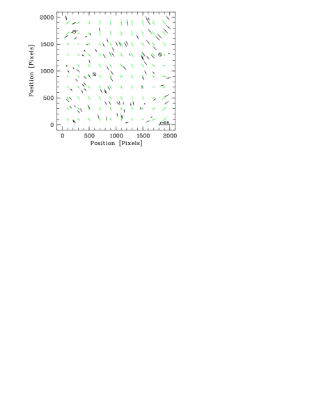
Figure 1: Visualisation of a spatially variable PSF. Each vector corresponds to one star found in the image, its length given by the ellipticity and its orientation by the position angle of the major axis. Note the well-ordered pattern which makes analytic modelling straightforward, the resulting model grid is overlaid in light gray. Circles mark the stars of Fig. 2 in same order from left to right. Image size is 13$.\mkern-4.0mu^{\prime}$3 across.

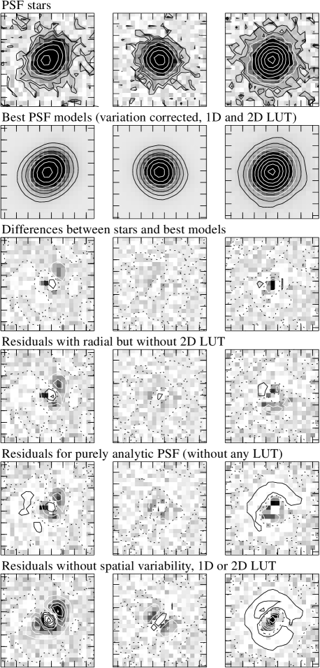
Figure 2: Modelling the PSF variations. Top row: Logarithmic contour plots and grayscale plots of three example stars taken from different locations in the same image. Slightly varying ellipticities can be traced even by eye. Second row: best models with modelling of spatial variation, one- and two-dimensional lookup table corrections. Third and subsequent rows: Residuals after subtracting decreasingly elaborate PSF models from each star. Contours are linear and symmetric around zero (dotted line). Coordinate tickmarks in all plots are 0$\aas@@fstack{\prime\prime}$5 apart.

Table 1: Quality of different PSF models with or without correction of spatial variability, one- and two dimensional LUTs. For the stars shown in Fig 2 we tabulate the rms of residuals in per cent of total stellar flux and the reduced $\chi^{2}$.

Correction			PSF 1		PSF 2		PSF 3
var.	1d.	2d.	$\Delta F$	$\chi^{2}_{\mathrm{r}}$	$\Delta F$	$\chi^{2}_{\mathrm{r}}$	$\Delta F$	$\chi^{2}_{\mathrm{r}}$
+	+	+	0.066	2.2	0.059	1.6	0.029	1.7
+	+	–	0.095	2.6	0.060	1.7	0.034	1.8
+	–	–	0.101	2.9	0.077	1.8	0.039	2.3
–	–	–	0.166	6.3	0.096	2.2	0.060	3.7

2.2.2 Analytic models

To describe the radial PSF shape we have adopted Moffat’s (1969) PSF parameterisation, given in a modified form in Eqn 1 below. We find that this profile provides a reasonable fit to the PSF for several different datasets obtained in both optical and NIR domains. Note that the Moffat parameter $\beta$, which basically controls the kurtosis of the profile (larger $\beta$ implying a more peaked profile with weaker wings) has to be included as a free parameter, as we often find best-fit $\beta$ values significantly different from the canonical value of 2.5. Moffat’s original description has been reformulated to use $r_{1/2}$ as the radius which encloses half the total flux:

$$F_{\mathrm{PSF}}(r) \>=\> F_{0,\mathrm{PSF}}\,hscpdes\left[\,1+\frac{r^{2}}{r_{1/2}^{2}}\left(2^{1/\beta}-1\right)\right]^{-\beta}$$ (1)

Other analytic forms are conceivable, though the number of free parameters should not be increased, as this requires to increase the lower flux limit of acceptable stars which in consequence will decrease the number of sampling points of the spatial PSF variation. Instead, deviations between the analytic shape and the Moffat prescription can be handled by a lookup table, described in the next section.

The azimuthal PSF shape is assumed to be elliptical, thus requiring a semimajor axis $a$, a semiminor axis $b$, and a position angle $\phi$ as additional parameters to specify the model. We do not use these parameters directly, but transform them into

$$a_{x}^{2} = \frac{a^{2}(1-\epsilon)^{2}}{1-\epsilon(2-\epsilon)\cos^{2}\phi}$$

$$a_{y}^{2} = \frac{a^{2}(1-\epsilon)^{2}}{1-\epsilon(2-\epsilon)\cos^{2}(\phi+\pi/2)}$$ (2)

$$a_{xy} = \frac{2-\epsilon(2-\epsilon)\left(1+\sin 2\phi\right)}{b^{2}}-\frac{a_{x}^{2}+a_{y}^{2}}{a_{x}^{2}a_{y}^{2}}$$

where $\epsilon=1-b/a$. With these provisions and assuming for simplicity the centroid to be at $(0,0)$, the PSF shape in each pixel $(x,y)$ is given by

$$F_{\mathrm{PSF}}\>=\>F_{0,\mathrm{PSF}}\,\left[\,1+\left(\frac{x^{2}}{a_{x}^{2}}+\frac{y^{2}}{a_{y}^{2}}+a_{xy}\,xy\right)(2^{1/\beta}-1)\right]^{-\beta}.$$ (3)

A similar expression for the PSF was already employed successfully in crowded field photometry packages such as DAOPHOT (Stetson, 1987), and we simply adopted that concept to our needs. Its chief benefit lies in the fact that variations in position angle over the field, even a complete flip of orientation, correspond to secular changes in the $a_{x}$, $a_{y}$, $a_{xy}$ parameters. This fact enables us to use simple bivariate polynomials to describe the variation of parameters over the field of view, i.e. expressions of the form

$$a_{x}(x,y) = c_{0}+c_{1}x+c_{2}y+c_{3}xy+c_{4}x^{2}+c_{5}y^{2}+\dots$$

$$a_{y}(x,y) = d_{0}+d_{1}x+d_{2}y+\dots$$ (4)

$$a_{xy}(x,y) = \dots$$

The actual process to establish a complete PSF model runs as follows: First the suitable stars are selected. The brightest stars are modelled individually with a full five-parameter PSF model (Eqn 3), with the aim to find a best $\beta$ for the dataset. Once this is done, $\beta$ is fixed for all subsequent PSF fits, i.e. we do not allow $\beta$ to vary spatially.

In a next step we fit four-parameter models to all stars, using the modified downhill simplex described in detail in the next section. This results in a table of PSF parameters at various positions $(x_{i},y_{i})$ in the image frame. If the parameters are consistent with being constant over the frame, or if the scatter is much larger than any possible trend, the simple average is taken, otherwise a least-square bivariate polynomial is computed. We have currently implemented polynomial orders between 1 (bilinear) and 3 (bicubic). The degree which fits best is taken for the final PSF model, with the additional condition that the gradient of the polynomial should be small in the vicinity of the AGN. Extremely ill-fitting stars (and undetected binaries, galaxies etc.) are iteratively removed from the table and do not contribute to the variation fit.

In the example of Fig. 1 we plotted position angle and ellipticity of all usable stars along with a grid of reconstructed values. The number of stars in the example is high, but not exceedingly so. The stability of the process allows us to use stars significantly fainter than the quasar which are of course much more numerous. In our applications like those presented in section 4 we typically find 20 – 30 or so usable stars per image.

2.2.3 Lookup table correction

For cases where the quality of the PSF determination is critical, i.e. for data with bad seeing or compact hosts, the analytic representation of the PSF may be an over-simplification. Without giving away the advantages of the analytic description, we can apply two second-order corrections in the form of empiric lookup tables (LUTs):

$$F_{\mathrm{PSF,corr.}}\>=\>F_{\mathrm{PSF}}+N\left[L_{1}(r_{n})+L_{2}(x,y)\right]$$ (5)

with $r_{n}=r/r_{1/2}$ being the normalised radius, $r$ the elliptical radius as described in Eqn 8 and $N$ a scaling factor for the LUTs. Here we distinguish between the case of azimuthally symmetric errors and that of errors with more complicated or no symmetries:

The one-dimensional (radial) LUT $L_{1}$ contains those corrections that show the same symmetry and variation as the model PSF itself. It describes the intrinsic radial shape difference between the simple analytical model and the more complicated PSF and can be expressed as an additive term in Eqn 1.

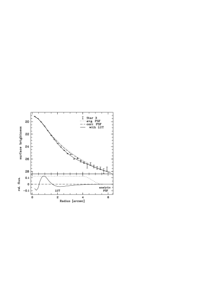
Figure 3: Comparison of profiles with and without radial LUT. As example we take star 3 from Fig 2. Top panel shows profiles of the star (dots), the best-fitting model with LUT (full line) and without LUT (dashed). Bottom panel shows the radial lookup table (solid line) in per cent of the total flux, together with a scaled transition function $f(r)$ (dotted line) defining the outer LUT boundary.

In practice, $L_{1}(r_{n})$ is obtained by assessing the residuals of PSF stars, normalised to unit integral flux, after subtraction of the best fitting analytic model. Of those we compute radial profiles spaced in equidistant fractions of $r_{1/2}$.

For each radial bin we then average the individual residual profile value for all stars. Due to the previous normalisation and azimuthal averaging, this process is now independent of the spatial PSF variation. The resulting lookup table $L_{1}(r_{n})$ can then be used to correct the symmetric radial errors according to Eqn 5. In Fig 3 we have done this for the image presented in Fig 1. The purely analytic model can describe the profile only up to a certain degree. To improve the fit (most conspicuously needed between two and four arcseconds) we add the radial LUT, scaled by the total stellar flux, in a range where it can be determined with high S/N. Note that the scale of the LUT is linear while the profiles are plotted logarithmically, the LUT is hence mostly needed in the centre, not in the wings.

In the next step we apply this global correction to all stellar models, adapted to their individual model geometry, and again record the residual images. Averaging these residuals after flux normalisation yields a two-dimensional array $L_{2}(x,y)$ which is just the desired lookup table. To avoid sampling errors, the images should be resampled to have the same subpixel centroids.

The quality of both corrections is necessarily a function of the number of stars available, and of their S/N ratios. In any case, for both the one- and two-dimensional LUT there exists a radius beyond which Poisson noise will dominate. The LUTs should be truncated at this radius to avoid the introduction of additional noise. To avoid artefacts at the cut-off radius, we apply a smooth transition. For this we define a transitional annulus [$r_{1}$:$r_{2}$] where $\tilde{L}=f(r)L(r)$ with $f(r)$ a third order polynomial for which holds:

$$f(r_{1}) = 1$$

$$f(r_{2}) = 0$$

$$f^{\prime}(r_{1}) = f^{\prime}(r_{2})=0\,.$$

The transition radii are determined interactively as the range where noise starts to dominate the LUT. An example of the transition function $f(r)$ is shown in Fig 3. Up to a radius of $4^{\prime\prime}$ we have $f(r)=1$, while within the transition annulus $f(r)$ decreases to 0. The effective $\tilde{L}$ is also plotted.

In Fig 2 we show the improvement in PSF fitting with each successive increase in model complexity. In the top three rows we plot logarithmic contours of three stars and the best-fitting models as well as linear contours of the resulting residuals. In the following rows we successively reduce the model complexity which leads to an increase in the residual structure as well as in the rms of the residual as shown in Table 1. Taken all corrections together we now have a high S/N-model of the PSF.

In order to estimate the accuracy of the above process, we adopted the ’leaving one out’ method from Duda & Hart (1973). We repeat the PSF determination but leave one star out. From the remaining stars we get a prediction of the PSF parameters at the star’s position which is independent from the star itself. We do this for all the stars and average the differences between predicted and measured PSF parameters. If the stars cover the field evenly this will be a good estimate for the uncertainty of the QSO PSF.

2.3 Image decomposition

2.3.1 Models

In order to describe the surface brightness distribution of QSO host galaxies we have restricted ourselves to the two most commonly used analytical prescriptions – an exponential Freeman (1970) law describing early type disc galaxies, and a de Vaucouleurs (1948) ‘$r^{1/4}$’ law describing spheroidals, applicable to elliptical galaxies and disc galaxy bulges:

$$F_{\mathrm{disc}}(r) = F_{\mathrm{disc},0}\exp\left(-1.68\,\frac{r}{r_{1/2}}\right)$$ (6)

$$F_{\mathrm{sph}}(r) = F_{\mathrm{sph},0}\exp\left[-7.67\,\left(\frac{r}{r_{1/2}}\right)^{1/4}\right]$$ (7)

where the ‘radius’ $r$ is a function of $x$ and $y$:

$$r^{2}\>=\>\frac{1-\epsilon(2-\epsilon)\cos^{2}(\alpha-\phi)}{(1-\epsilon)2}\left(x^{2}+y^{2}\right)\>,$$ (8)

with $\tan\alpha=y/x$. (Exponential bulges in late-type spirals are currently not modelled as these are not known to harbour significant nuclear activity). Thus, each galaxy model contains four independent parameters: The semimajor axis $a$ for which holds that $r(a)=r_{1/2}$; the ellipticity $\epsilon=1-b/a$; the position angle of the major axis, $\phi$; and the total flux $F=\int F(r)\>\mathrm{d}r\>\mathrm{d}\alpha$. Notice that we avoid to use the ill-constrained central surface brightness as a fit parameter. It is well known that the determination of effective radius and central surface brightness is strongly degenerate in the presence of measurement errors (e.g. Abraham et al., 1992), and that the total flux $F_{0}$ is much better constrained than either of these parameters. This issue will be addressed again in Sect. 3 below, in particular in Figs 6 and 7.

To summarise, a typical model will contain either five or nine parameters: four for each galaxy component, plus a point source scaling factor for the AGN. However, we have also implemented an option to keep individual parameters at a fixed value, so that the above numbers give the maximum number of parameters.

2.3.2 Convolution

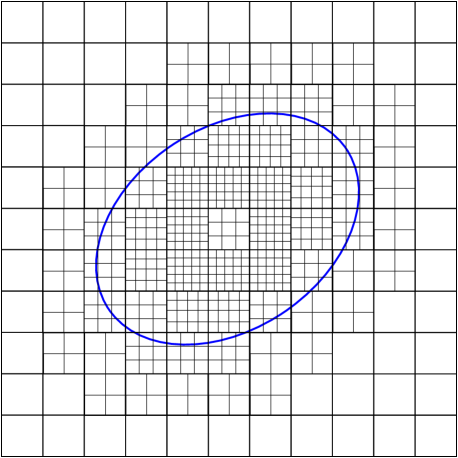
Figure 4: Illustration of the adaptive subxpixelling. Each pixel with a gradient larger then a threshold value is divided into subpixels. These subpixels itself are divided as long the gradient is still too large. The size of the original pixels is maintained in the outer parts. The ellipse represents this object’s half-light isophote.

Although both PSF and galaxy are represented by analytic functions, the nonzero ellipticities demand that the convolution be evaluated numerically. In numerical convolution, sampling plays an important role: strictly speaking, we have to distinguish between (a) the function value at given $x,y$; (b) the PSF-convolved value; (c) the image value sampled into a rectangular pixel grid. These values will be similar only in areas of small gradients in the surface brightness distribution; close to the centre, the galaxy light has to be sampled on a much finer grid in order to avoid large numerical errors. On the other hand, a highly oversampled pixel grid leads to a substantial increase in computing time and is therefore inefficient. It is also not required in the outer regions.

Our adopted solution uses the local gradient in the unconvolved image to adjust the degree of oversampling, as illustrated in Fig 4. This adaptive subpixel grid is determined at the beginning of each fitting subprocess (see below). Whenever the model parameters change substantially, the grid is recomputed and the fitting process is resumed with this new grid.

2.3.3 The fitting process

The model parameters are iteratively adjusted by minimizing $\chi^{2}$ with the downhill simplex method (Press et al., 1995). Here, the $\chi^{2}$ values are based on variance frames associated with each image, which may also contain information about regions that are to be left out of the fitting process.

In order to accelerate and stabilise the minimization, the parameter space is transformed to achieve ‘rounder’ $\chi^{2}$ valleys. We use the following transformation recipes: $\epsilon$ is substituted by $\epsilon^{\prime}\equiv\log(1-\sqrt{1-\epsilon^{2}})$, and $F$ is substituted by $F^{\prime}\equiv\log(F+O)$. As a byproduct, this transformation automatically ensures that F has a lower acceptable bound $-O$. Note that $O=0$ (i.e. demanding $F>0$) is not always a good choice; in the case of a faint or undetectable host galaxy and in the presence of noise, slightly negative values of $F$ must be permitted.

A crucial part of the algorithm is its subdivision into successive minimization substeps in order to avoid trapping in local minima. Whenever a $\chi^{2}$ minimum is found, the process is restarted at the same location in parameter space, probing the environment for a further decrease in $\chi^{2}$-values. Additional restarts are launched when the change in parameters requires a reevaluation of the subpixelling grid. Only when even repeated restarts yield no improvement in $\chi^{2}$, the entire process is considered to have found a global minimum. This way we can usually avoid to be trapped in shallow local minima or regions of small curvature.

Fitting the full set of nine parameters is only useful for data with excellent spatial resolution, providing significant independent constraints for AGN, disc, and bulge components. There are various ways to reduce the number of fitting parameters; besides fitting just one galaxy model, we have included an option to keep parameters at a fixed value. This is useful e.g. in the analysis of multicolour data where certain structural parameters might be well-constrained in one dataset (e.g., HST) which then can be used to increase the modelling fidelity of images taken in other bands.

Table 2: Overview over our simulations. The input parameters are total counts $F$ (in units of detector photoelectrons) and half-light radii $r$. Corresponding absolute magnitudes $M$ and linear radii $r$ [kpc] are also listed for comparison. For details see text and Table 3.

Dataset	$F_{\mathrm{nuc}}$	$F_{\mathrm{disc}}$	$F_{\mathrm{sph}}$	$r_{\mathrm{disc}}$	$r_{\mathrm{sph}}$	$-M_{R,\mathrm{nuc}}$	$-M_{R,\mathrm{disc}}$	$-M_{R,\mathrm{sph}}$	$r_{\mathrm{disc}}$	$r_{\mathrm{sph}}$
	$10^{5}$ [e-]	$10^{5}$ [e-]	$10^{5}$ [e-]	[arcsec]	[arcsec]				[kpc]	[kpc]
med $z|_{s}$	10	–	2.5	–	1.3	24.5	–	23.0	–	10.0
med $z|_{m}$	11–7.8	–	11–0.8	–	1.2–4.1	24.5	–	22.0–24.5	–	8.7
med $z|_{e}$	10	–	2.5	–	1.3–10.8	24.5	–	23.0	–	10.0–78.4
low $z|_{M}$	10	1.0–20	1.0–20	6.0	3.0	24.2	21.7–25.0	20–22.5	5.0	2.5
low $z|_{R}$	10	1.0	1.0	3.0–8.0	1.5–6.0	24.2	21.7	21.7	2.5–6.8	1.3–5.0

3 Simulations

To test the reliability of the AGN decomposition process, we constructed extensive sets of simulated galaxies. As the multitude of instruments and objects prevents a test for the full range of possible data, we limit the test to two rather different sets which both closely resemble certain observational data recently obtained by us. One the one hand, we consider a set of low redshift AGN observed with a 1.5 m telescope. On the other hand, we consider the case of medium to moderately high redshift QSOs (up to $z\simeq 1$), observed with a 4 m class telescope. These simulations resemble the examples described in Sect. 4.1 of this paper. These two simulated datasets will henceforth be referred to as ‘low $z$’ and ‘med $z$’. Input properties are listed in Table 2.

We have thus constructed a test bed for two very different configurations. The low-redshift objects were created using various combinations of three components (disc, spheroid and a nuclear source), and among these objects we expect to find and retrieve all Hubble types. For the medium and high redshift data we expect elliptical galaxies to dominate the host galaxy population. In this case the objects are compounds of only a spheroidal and a nuclear component, and we attempt no more than reclaiming the properties of these two components, concentrating on luminosities and scale lengths. In this paper we do not investigate the influence of inclination on the decomposition process.

Both simulated sets were created using the same radial profiles and isophotal shapes that we used to compute the model galaxies during the fitting process. To account for observational errors we added artificial shot noise. The sets were then treated in the same way as real observational data. In order to avoid confusion between errors in the modelling of the spatial PSF variations and the fitting of galaxy and AGN, we assumed the PSF to be shift-invariant.

3.1 Medium-redshift simulations

We start with the medium-redshift simulations as these were fitted with the conceptually simpler two-component models. The first subset contains images of only a single galaxy, but ‘observed’ numerous times, i.e. with several different noise realisations, and with different centroid positions with respect to the pixel grid (dataset ‘med $z|_{s}$’, for ‘single redshift’, in Table 2). The input galaxy is a typical bright elliptical galaxy with half-light radius $r_{1/2}=10$ kpc, an absolute luminosity of $M_{R}=-{24.5}$ at a redshift of $z=0.6$, with a nucleus four times brighter than the host galaxy.

Figure 5: Two example model galaxies. In the top row we show the composite model and the single components of the ‘med $z|_{s}$’ model,in the bottom row the same is done for the ‘low $z|_{M}$’ model with the weakest host. Scales and cuts are held constant for each redshift.

To compute realistic flux and background levels, we used the exposure time calculator for the ESO-NTT and its multi-mode instrument EMMI, assuming a pixel size of $0\aas@@fstack{\prime\prime}27$ and a total exposure time of 500 s per simulated image. In order to specify the background level, we assumed the data to be obtained in the $V$ band. The adopted PSF has a width of $0\aas@@fstack{\prime\prime}8$ FWHM, compared to $r_{1/2}=1\aas@@fstack{\prime\prime}33$ for the galaxy.

Fitting the simulated images of this dataset, we found that we are able to reclaim the original host galaxy magnitude with an uncertainty of only 0.02 (1$\sigma$). This is shown in more detail in Fig 6, which also illustrates the well-known fact that the half-light radius is less accurately recovered. However, with an uncertainty of 9 per cent in $r_{1/2}$ we are still able to give a solid estimate of the galaxy size, even at this redshift and with a host galaxy only slightly more extended than the PSF.

In the second dataset (‘med $z|_{m}$’, for ‘multiple redshifts’), we placed the same galaxy at four different redshifts ($z=0.1$, 0.2, 0.4, 1.2) and changed the galaxy flux such that the ratio nucleus/galaxy takes three different values (10:1, 4:1, 1:1). To enable a fair comparison, the exposure time in each case was adjusted to yield the same S/N for all redshifts (cf. Table 3), and the underlying spectrum was assumed to be flat, i.e. we have the same luminosity in all the spectral bands. This latter assumption is obviously unphysical, but acceptable for our illustration purposes as the main free input parameters are the nuclear flux and the nuclear/host flux ratio.

For each configuration we generated images with several different noise realisations and fitted those independently. The results show clearly and not surprisingly that the accuracy of recovering the input parameters depends on redshift (see Fig 7). But even in the case of the most unfavourable redshift, $z=1.2$ and the highest nuclear/host ratio, the reconstructed host galaxy luminosity has an rms scatter of less than 0.15 mag (1$\sigma$). Again, the half-light radii are less accurately determined. Ellipticity and position angle were held constant during these simulations ($\epsilon=0.4$, PA = 20^∘). Fitted values agreed on average with the model values with scatters below 2 per cent in $\epsilon$ and $3^{\circ}$ in PA except for the faintest models where it rose to 20 per cent and $8^{\circ}$ for the faintest. This held for all redshifts except the lowest where the scatter was significantly smaller.

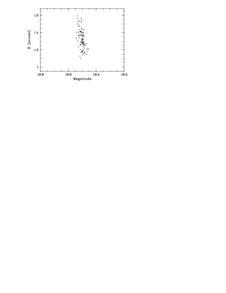
Figure 6: Results for the ‘med $z|_{s}$’ simulation, featuring different noise realisations and subpixel locations. Each dot represents the result of fitting one particular image. The circle indicates the average of the fitted values, and the cross denotes the ‘true’ input value. The nucleus is brighter than the host galaxy by 1.5 mag. The scatter of extracted parameter values (1$\sigma$) is 0.02 for the magnitude and 9 per cent for the radius.

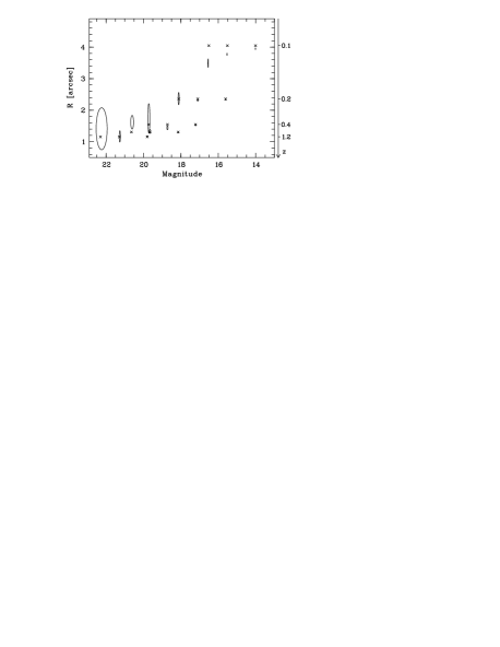
Figure 7: Results for the ‘med $z|_{m}$’ simulations, involving four different redshifts. Crosses represent the input values, and the ellipses approximately delineate the scatter of the extracted parameter values, with a minor semiaxis of 2$\sigma$ in magnitude and a major semiaxis of 1$\sigma$ in radius. The magnitude of the nuclear component is equal to that of the brightest host galaxy at each redshift. Values are given in arcseconds and $R$-band apparent magnitudes.

3.2 Influence of external parameters

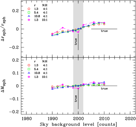
Figure 8: Dependence of recovered radii (top) and magnitudes of the galaxy (bottom) on the on the accuracy of the background determination. Instead of using the true value (marked with a vertical bar) we used offset values for the sky background to fit the data. The shaded area is the range of the typical background uncertainty.

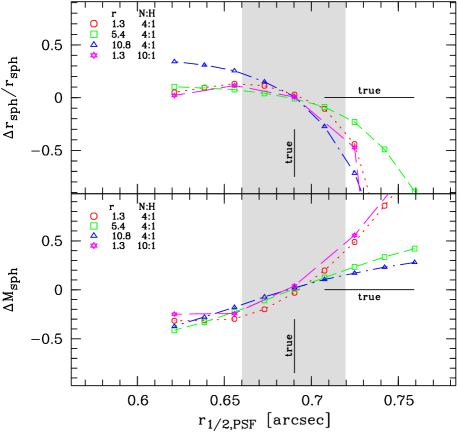
Figure 9: Dependence of recovered radii (top) and magnitudes of the galaxy (bottom) on accuracy of the half-light radius of the PSF.

In the simulations we assumed that we know the true value of the sky background and the PSF parameters. In reality these are afflicted with uncertainties. To test their influence we created a set of models (‘med $z|_{e}$’, for ‘external’) similar to the ‘med $z|_{s}$’ simulations (which have $z=0.6$ and a nucleus four times brighter than the host) but with three different galaxy radii ($r_{1/2}=1\aas@@fstack{\prime\prime}33,5\aas@@fstack{\prime\prime}4,10\aas@@fstack{\prime\prime}8$) in order to resemble observations typical for our group.

These models were fitted using deliberately wrong values (one at a time) for the sky background, which is notorious for influencing the results, and the PSF half-light radius $r_{1/2}$ which appeared to be the most critical parameter. For each configuration we generated a number of different noise realizations and computed the average values of recovered host galaxy radius and magnitude.

In Figs 8 and 9 the results can be compared. While in the typical range of errors the uncertainties induced by an uncertain background are almost negligible for the magnitude and below 5 per cent for the radius, the accuracy of the determined PSF half-light radius is essential. Errors are as large as 0.5 magnitudes or 50 per cent for the radius here.

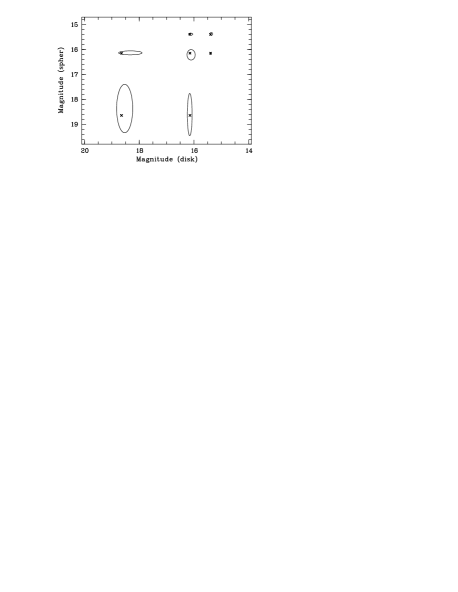
Figure 10: Results for the ‘low $z|_{M}$’ simulation, showing the accuracy of reclaiming component luminosities in three-component fits. The error ellipses have semiaxes of 2$\sigma$ in magnitude. The nuclear component has a magnitude of 16.15 for all objects.

We also created models which have nuclei 10 times brighter than the host galaxy, similar to the ‘worst case’ in the $z=1.2$ ‘med $z|_{m}$’ models. Fitting those with offset values for the background and the PSF half-light radius, we find the systematic errors to be comparable to those of the ‘typical’ models (see Figs 8 and 9). In the background test the larger statistical errors introduced by the fitting process (see Sect. 3.1 and Fig 7) become visible. This is less visible in the PSF half-light radius test, as the different nuclear-to-host relation play a less prominent role. Here, the error of the nucleus dominates as long as it is notably brighter than the galaxy.

3.3 Low-redshift simulations

For well resolved AGN host galaxies a three-component fit may be more appropriate. In our low-redshift sample, the host galaxies are of all Hubble types and their morphology can be easily resolved even with small telescopes as we will show in the next section. To test the three component fitting, we generated a dataset to match those observations.

We simulated galaxies with both a disc and a spheroid and a bulge-to-total ($b/t$) flux ratio between 0.1 and 0.9. The ratio between nuclear and galactic light was varied between 5:1 and 1:4 (set ‘low $z|_{M}$’ for ‘magnitude variation’ in Table 2). The half-light radii were set to typical values found in our observed sample. All galaxies are azimuthally symmetric, no late-type features like bars or spiral arms were added.

Note that the simulations were designed to match the observations in integrated flux and apparent radii. Values in the table are given for a template observation of 840 s exposure time (on a 1.5 m telescope) and a redshift of 0.019, which was also used to compute the level of noise of 800 e^-/Pixel at a pixel size of 0$\aas@@fstack{\prime\prime}$39. We assumed a seeing of 1$\aas@@fstack{\prime\prime}$6 (FWHM), which is rather poor but unfortunately was typical for our observations.

Fig 10 shows the results of the fits. The property dominating the uncertainty is the flux ratio between nuclear component and the galaxy (moving from lower left to upper right in Fig 10 decreases this ratio). The bulge magnitude is more affected by this than the disc magnitude, which is easily explained by the lower half-light radii of the bulge component, which is thus harder to be distinguished from the nucleus. The 1$\sigma$ uncertainty grows from 0.03 mag for a ratio of 1:2 (nuclear to spheroidal flux) to 0.46 mag for a ratio of 10:1); the corresponding values for the disc component are 0.02 mag at 1:2 and 0.2 mag at 10:1.

In order to probe how well galaxy sizes can be recovered with these multicomponent fits, we varied the radii of both components between 1$\aas@@fstack{\prime\prime}$5 and 6$\aas@@fstack{\prime\prime}$0 (bulge) and 3$\aas@@fstack{\prime\prime}$0 and 8$\aas@@fstack{\prime\prime}$0 (disc) but left the fluxes unchanged, with the flux ratio set to the worst-case value of 10:1 for each component (dataset ‘low $z|_{R}$’, for ‘radius variation’). Fig 11 shows that even when the nucleus dominates over the galaxy, the relative error in the determination of the half-light radius is reasonably low ($\sim 5$ per cent for the disc and $\sim 20$ per cent for the spheroidal component).

No special simulations were done for ellipticity and position angle. Within the above simulations, where both had constant values ($\epsilon=0.33$, $\phi_{\mathrm{sph}}=22^{\circ}$, $\phi_{\mathrm{dis}}=37^{\circ}$), they were on average fitted well with scatters below 2 per cent in $\epsilon$ and $2^{\circ}$ in PA. Again for the faintest galaxies the scatter rose to 6 per cent and $4^{\circ}$ and as high as 25 per cent and $6^{\circ}$ if the galaxy component was hidden by both a bright nucleus and a bright second galaxy component. We did not do specific simulations for other values of $\epsilon$ and $\phi$, but tests suggest that for larger values of $\epsilon$ both are determined even better, while for smaller values no large differences are expected, as the above case is already almost circular.

We conclude by stating that our simulations have yielded encouraging results. Total host galaxy luminosities can be reclaimed with high fidelity, and although half-light radii are less accurately constrained, there is no evidence for systematic errors. Recall that noise level, pixel sampling, and in particular seeing in these simulations were matched to our already existing data. It would be easy to design additional datasets obtained under better conditions, in which case a substantial improvement of measurement accuracy can be expected. We stress, however, the importance of individually tailored simulations in order to assess the potential and limitations of each observed dataset.

Table 3: Redshifts, apparent nuclear magnitudes, exposure times and resulting sky background contribution adopted as input for the simulations.

Set	$\>\>\>z$	$V$	$t_{\mathrm{exp}}$	BG
			[s]	[e-/Pixel]
low $z$	0.02	14.0	840	800
med $z$	0.1	14.3	10	40
med $z$	0.2	15.9	44	176
med $z$	0.4	17.5	200	800
med $z$	0.6	18.4	500	2000
med $z$	1.2	20.1	3100	12400

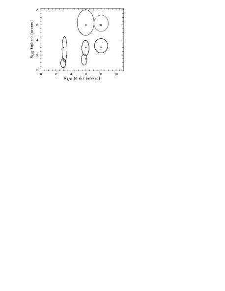
Figure 11: Results for the ‘low $z|_{R}$’ simulation, featuring three-component models with different half-light radii. Error ellipses have semiaxes of 2$\sigma$ of the radius (in arcseconds). All objects have a nuclear to total galactic flux ratio of 5:1 and a $b/t$ of 0.5. Radii are given in arcseconds.

4 Example applications

4.1 Samples and observations

As a first test case with real data, we have investigated two statistically complete samples of quasars and Seyfert 1 galaxies. The objects form subsamples of the Hamburg/ESO survey (HES, Wisotzki et al., 2000) and constitute quasars and Seyfert 1 galaxies with redshifts $z<0.35$ resp. $0.01<z<0.05$. Typical nuclear absolute magnitudes are around $M_{H}\simeq-27$ (medium redshift) and $M_{B}\simeq-21$ (low redshift).

All 13 low redshift objects were observed in the $R$ band using the ESO/Danish 1.54 m telescope on La Silla and its multi-purpose instrument DFOSC. The seeing during the three nights of observation was rather poor (1$\aas@@fstack{\prime\prime}$3–1$\aas@@fstack{\prime\prime}$8), but due to their low redshifts all of our objects were spatially well resolved.

The 42 med-z quasars were observed in $H$ band during two nights using the ESO NTT telescope with the SOFI camera with a seeing of 0$\aas@@fstack{\prime\prime}$4–0$\aas@@fstack{\prime\prime}$8.

The images were reduced with standard procedures (debiasing, flatfielding) and flux-calibrated using standard star sequences taken in the same nights. For the infrared images the sky background / bias was determined using stacks of dithered on-target images. For analysis we shifted the images to same object centroids using subpixeling and coadded the images.

4.2 Modelling

The fitting of the data followed the procedure laid out in sections 2.2 and 2.3. The PSF determination for the low redshift observations was straightforward, as with the large field of view of the DFOSC detector (13$.\mkern-4.0mu^{\prime}$3 $\times$ 13$.\mkern-4.0mu^{\prime}$3) always a large number of stars were available in the image, at least 20 or 30. The field of view of SOFI is notably smaller (4$.\mkern-4.0mu^{\prime}$6 $\times$ 4$.\mkern-4.0mu^{\prime}$6) but as the images are also deeper the number of usable stars is again typically 20 or 30 and always greater than 12. Depending on the image, a second or third order polynomial could usually represent the variation to sufficient accuracy. Figs 1 and 2 were actually created from this data.

Figure 12: Two examples from the medium redshift sample at $z=0.18$ (top) and $z=0.32$. Left column: contour plots, with contour spacings of one magnitude. Middle: Azimuthally averaged profiles, with dots representing the observed data and the solid line denoting the overall fit. Dashed, dotted, and dashed-dotted lines correspond to the disc, spheroidal, and nuclear model components, respectively. Right: residual images after subtraction of all model components. Cut levels are set at $\pm$ the value of the outermost isophotes shown in the contour plots. White/black areas indicate regions where the model is brighter/fainter, respectively, than the data. Units are arcseconds in the contour plots and mag$/\sq^{\prime\prime}$ against arcseconds in the profiles.

Some preparatory work before the host galaxy modelling involved fine-tuning of the local sky background near each AGN using growth curves, and masking all features in the frames that clearly do not belong to the object. The maximum fitting radius was set to an ellipse containing 99.5 per cent of the total object flux. The contour plots in Figs 12 and 13 have been made just large enough for this ellipse to fit in.

Good initial parameter estimation is very important to avoid local $\chi^{2}$ minima located at parameter combinations very different from those near the global minimum. At least with the simplex method it is difficult to leave such a minimum, once trapped in it. We estimated initial parameters in the following way: We first determined the isophotal shape of the disc component (nearly always the most extended component) by fitting ellipses to the outermost isophotes. The scale length and total flux was then obtained from fitting an exponential law to the outermost part of the surface brightness profile. The determination of the bulge parameters was done likewise, but using the original image with a convolved disc component subtracted. Finally the remaining central flux was attributed to the nucleus. If any of these steps led to unsatisfactorily strong residuals, the process was repeated in a different order (first spheroid, then disc). The parameter values obtained from this procedure were used as initial guesses, enabling us to start the full three component fitting for the low redshift sample as well as to decide which galactic component to use in a two component fit for the medium redshift sample. In only five cases the resolution of the medium redshift images was good enough to allow a three component fit.

The quality of each fit was investigated manually by checking the resulting profiles, residual images (such as those shown in Fig 12), the sequence of $\chi^{2}$ values, and the plausibility of the parameters obtained. If a fit was not satisfactory, i.e. leading to strong residuals or to discrepancies with the object’s profile which could not be attributed to prominent features in the galaxy, we spent more effort in estimating good initial conditions, or imposed additional constraints in the form of boundary conditions to ensure that the fitting results corresponded to physically meaningful components. For a few objects the three component fit suggested that two components might be sufficient to model the light distribution. For these we repeated the fit with only two components and selected that if the fit was satisfactory. We comment on a few such cases below.

For the three low redshift objects where just a nuclear and a disc component were required we estimated an upper limit for the bulge luminosity by adding compact artificial spheroids ($r_{1/2}=1,5,10$ kpc) with successively decreasing fluxes. These images were fitted with both a nucleus plus disc and with a three components model. The faintest spheroid for which a three component fit is preferred (i.e. has a significantly lower reduced $\chi^{2}$) is then taken as limit for the detection of a spheroid in that object. We did not determine limits for the bulge size, as the sensitivity on the size drastically reduces towards low galaxy fluxes (see above).

For one object, HE 1348$-$1758, which did not show any nuclear component, an upper limit was estimated in a similar fashion by adding an artificial nucleus.

Figure 13: Two examples from the low redshift sample. Notation is as in Fig 12

Figure 14: Two examples of unsatisfactory fits, requiring user intervention. For HE 1017–0305 a excessively large spheroid is fit due to surplus in surface brightness at 6″to 9″. For HE 1348–1758 we forced an unresolved nuclear source instead of a spheroid. Notation is as in Fig 12

4.3 Results

For all of our objects we were able to obtain satisfactory fits. Some examples of objects, profiles, and residual images after subtracting the models are presented in Figs 12 and 13.

In some of the residual images, little or no structure was left at the location of the galaxies. This is the case for HE 1348$-$1758 and HE 0914$-$0031. In the majority of the objects, strong features were present, mainly indicating the limitations of the azimuthally symmetric models. These morphological features will also influence the fit itself and may render it less reliable. An example is HE $1017-0305$, where a pair of counter-coiled spiral arms, or tidal features, causes a significant surplus of flux at larger radii which mimics the contribution of an unphysically large spheroidal component. The resulting fit is shown in Fig 14. A better fit is obtained when the fitting area is restricted to regions unaffected by the extended arms (Fig13, top line).

The magnitudes of the components were computed from the best-fitting model parameters, which already contain the total fluxes for each component. Other methods are possible such as using the obtained nuclear model to subtract the nuclear source and then determining the galaxy flux from growth curves of the remaining host galaxy. This method yields a more precise nuclear-to-ratio as it is strictly flux-conserving. For the goal of computing the fluxes of several galaxy components separately, this is not as straightforward. For our data we tested and compared both methods and found that they agree extremely well. Fluxes taken from the model parameters are, on average, brighter by 2 per cent, with an rms scatter of $\pm$ 4 per cent.

Magnitude errors were estimated using dedicated simulations (described in the section 3) by interpolating the uncertainties of the two most similar simulated objects. We did not include error estimates concerning the systematic differences between fitted and observed profile but included the uncertainties raised by the errors of PSF radius and the sky background level. In Fig 15 we plot magnitudes of the host galaxy and the nuclear component along with their uncertainties.

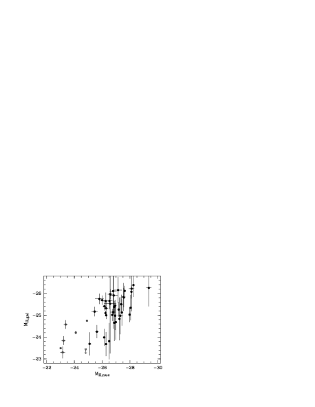
Figure 15: Nuclear versus spheroid luminosities. The circles are from the medium redshift, squares from the low redshfit sample. Errorbars are based on dedicated simulations. The arrow indicates an upper limit for the speroid.

5 Conclusions

We have presented a versatile method to describe the light distribution of quasar host galaxy images. Particular attention was paid to a careful quantitative modelling of the PSF underlying the quasar images, in order to make the decomposition of the quasar into host galaxy and nuclear components as reliable as possible, even using non-optimal observing material.

The simulations shown in the present paper show that our method is well suited to derive accurate and unbiased host galaxy luminosities with realistic error estimates.

We demonstrated the usefulness of the method for two small samples of local Seyfert galaxies and medium redshift quasars. The latter was observed with the main intention to constrain the host galaxy luminosity distribution function. Preliminary results were presented by Wisotzki et al. (2001) a more detailed account is given by Kuhlbrodt (2003).

We have already applied the algorithm to other data. For a sample of $\sim 20$ low-redshift quasars ($z<0.2$), which we observed in several optical and near-infrared wavebands, we have derived spectral energy distributions and stellar population descriptions (Jahnke et al., 2003). Additional applications can easily be conceived.

6 Acknowledgements

This work was supported by the DFG under grants Wi 1369/5–1 and Re 353/45-3. We made use of observing time at ESO with the programme 61.B-0300. KJ acknowledges support by the ‘Studienstiftung des Deutschen Volkes’.

References

- Abraham et al. (1992) Abraham R. G., Crawford C. S., McHardy I. M., 1992, ApJ, 401, 474
- de Vaucouleurs (1948) de Vaucouleurs G., 1948, Ann. Astrophys., 11, 247
- Duda & Hart (1973) Duda R., Hart P., 1973, Pattern Classification and Scene Analysis. Wisley
- Falomo et al. (2001) Falomo R., Kotilainen J., Treves A., 2001, ApJ, 547, 124
- Freeman (1970) Freeman K. C., 1970, ApJ, 160, 812
- Jahnke et al. (2003) Jahnke K., Kuhlbrodt B., Wisotzki L., 2003, astro-ph/0311123
- Kuhlbrodt (2003) Kuhlbrodt B., 2003, PhD thesis, Universität Hamburg
- Kukula et al. (2001) Kukula M. J., Dunlop J. S., McLure R. J., Miller L., Percival W., Baum S. A., O’Dea C. P., 2001, MNRAS, 326, 1533
- Lehnert et al. (1999) Lehnert M. D., van Breugel W. J. M., Heckman T. M., Miley G. K., 1999, ApJS, 124, 11
- McLeod & McLeod (2001) McLeod K. K., McLeod B. A., 2001, ApJ, 546, 782
- McLure et al. (2000) McLure R. J., Dunlop J. S., Kukula M. J., 2000, MNRAS, 318, 693
- McLure et al. (1999) McLure R. J., Kukula M. J., Dunlop J. S., Baum S. A., O’Dea C. P., Hughes D. H., 1999, MNRAS, 308, 377
- Moffat (1969) Moffat A. F. J., 1969, A&A, 3, 455
- Press et al. (1995) Press W. H., Teukolsky S. A., Vetterling W. T., Flannery B. P., 1995, Numerical recipes in C, 2nd edn. Cambridge University Press
- Ravindranath et al. (2001) Ravindranath S., Ho L. C., Peng C. Y., Filippenko A. V., Sargent W. L. W., 2001, AJ, 122, 653
- Ridgway et al. (2001) Ridgway S. E., Heckman T. M., Calzetti D., Lehnert M., 2001, ApJ, 550, 122
- Schade et al. (1996) Schade D., Lilly S. J., Le Fevre O., Hammer F., Crampton D., 1996, ApJ, 464, 79
- Stetson (1987) Stetson P. B., 1987, PASP, 99, 191
- Wadadekar et al. (1999) Wadadekar Y., Robbason B., Kembhavi A., 1999, AJ, 117, 1219
- Wisotzki et al. (2000) Wisotzki L., Christlieb N., Bade N., Beckmann V., Köhler T., Vanelle C., Reimers D., 2000, A&A, 358, 77
- Wisotzki et al. (2001) Wisotzki L., Kuhlbrodt B., Jahnke K., 2001, in Márquez I., et al. eds, QSO Hosts and Their Environments Kluwer