Peak Energy–Isotropic Energy Relation in the Off-Axis Gamma-Ray Burst Model

Abstract

Using a simple uniform jet model of prompt emissions of gamma-ray bursts (GRBs), we reproduce the observed peak energy–isotropic energy relation. A Monte Carlo simulation shows that the low isotropic energy part of the relation is dominated by events viewed from off-axis directions, and the number of the off-axis events is about one-third of the on-axis emissions. We also compute the observed event rates of the GRBs, the X-ray-rich GRBs, and the X-ray flashes detected by HETE-2, and we find that they are similar.

1 Introduction

There is a strong correlation between the rest-frame spectral peak energy $(1+z)E_{\rm p}$ and the isotropic equivalent $\gamma$-ray energy $E_{\rm iso}$ of the gamma-ray bursts (GRBs). This relation ($E_{\rm p}$–$E_{\rm iso}$ relation) was first discovered by Amati et al. (2002), and recently extended down to lower energies (Atteia, 2003; Lamb et al., 2003b; Sakamoto et al., 2003), so that $E_{\rm iso}$ ranges over 5 orders of magnitude. A similar relation, the $E_{\rm p}$–luminosity relation is also found by Yonetoku et al. (2003), and both relations could become a new distance indicator. The geometrically corrected $\gamma$-ray energies $E_{\gamma}=(1-\cos\Delta\theta)E_{\rm iso}$ narrowly cluster around a standard energy $E_{\gamma}\sim 10^{51}$ ergs (Bloom, Frail, & Kulkarni, 2003a; Frail et al., 2001), so that the opening half-angle of the jet in the on-axis uniform jet model ranges 2.5 orders of magnitude. This means that if the low isotropic energy events correspond to the wide opening half-angle jet, the jet opening half-angle of the typical GRBs $\Delta\theta$ becomes less than $1^{\circ}$ (Lamb, Donaghy, & Graziani, 2003a). However such a small angle jet has difficulties in the standard afterglow models and observations. (see also Zhang & Mészáros, 2003).

The low-energy (low-$E_{\rm p}$) part of the relation consists of X-ray flashes (XRFs), that were identified by BeppoSAX (Heise et al., 2001) and other satellites (Strohmayer et al., 1998; Gotthelf et al., 1996; Hamilton et al., 1996; Arefiev, Priedhorsky, & Borozdin, 2003) and have been accumulated by HETE-2 (Barraud et al., 2003). Theoretical models of the XRF have been widely discussed (Yamazaki, Ioka, & Nakamura, 2003b): high-redshift GRBs (Heise et al., 2001; Barraud et al., 2003), wide opening angle jets (Lamb, Donaghy, & Graziani, 2003a), internal shocks with small contrast of high Lorentz factors (Mochkovitch et al., 2003; Daigne & Mochkovitch, 2003), failed GRBs or dirty fireballs (Dermer et al., 1999; Huang, Dai, & Lu, 2002; Dermer & Mitman, 2003), photosphere-dominated fireballs (Mészáros et al., 2002; Ramirez-Ruiz & Lloyd-Ronning, 2002; Drenkhahn & Spruit, 2002), peripheral emissions from collapsar jets (Zhang, Woosley, & Heger, 2003) and off-axis cannonballs (Dar & De Rújula, 2003). The issue is what is the main population among them.

We have already proposed the off-axis jet model (Yamazaki, Ioka, & Nakamura, 2002, 2003b). The viewing angle is the key parameter to understanding the various properties of the GRBs and may cause various relations such as the luminosity-variability/lag relation, the $E_{\rm p}$-luminosity relation and the luminosity-width relation (Ioka & Nakamura, 2001; Salmonson & Galama, 2002). When the jet is observed from off-axis, it looks like an XRF because of the weaker blue-shift than the GRB.

There are some criticisms against our off-axis jet model. The original version of our model (Yamazaki, Ioka, & Nakamura, 2002) required the source redshift to be less than $\sim 0.4$ to be bright enough for detection, conflicting with the observational implications (e.g., Heise, 2002; Bloom et al., 2003b). Yamazaki, Ioka, & Nakamura (2003b) showed that higher redshifts ($z\gtrsim 1$) are possible with narrowly collimated jets ($\lesssim 0.03$ rad), while such small jets have not yet been inferred by afterglow observations (Bloom, Frail, & Kulkarni, 2003a; Panaitescu & Kumar, 2002; Frail et al., 2001). The luminosity distance to the sources at $z\sim 0.4$ is $d_{L}\sim 2$ Gpc, which is only a factor of 3 smaller than that at $z\sim 1$ (corresponding to $d_{L}\sim 7$ Gpc). Thus small changes of parameters in our model allow us to extend the maximum redshift of the off-axis jets to $z\gtrsim 1$ even for $\Delta\theta\sim 0.1$. This will be explicitly shown in § 3. Therefore, off-axis events may represent a large portion of whole observed GRBs and XRFs since the solid angle to which the off-axis events are observed is large.

In this Letter, taking into account the viewing angle effects, we derive the observed $E_{\rm p}$–$E_{\rm iso}$ relation in our simple uniform jet model. This paper is organized as follows. In § 2 we describe a simple off-axis jet model for the XRFs. Then, in § 3, it is shown that the off-axis emission from the cosmological sources can be observed, and the $E_{\rm p}$–$E_{\rm iso}$ relation is discussed in § 4. Section 5 is devoted to discussions. We also show that the observed event rates of GRBs and XRFs are reproduced in our model. Throughout the Letter, we adopt a $\Lambda$CDM cosmology with $(\Omega_{m},\Omega_{\Lambda},h)=(0.3,0.7,0.7)$.

2 Prompt emission model of GRBs

We use a simple jet model of prompt emission of GRBs considered in our previous works (Yamazaki, Ioka, & Nakamura, 2003b; Yamazaki, Yonetoku, & Nakamura, 2003). We assume a uniform jet with a sharp edge, whose properties do not vary with angle. Note that the cosmological effect is included in these works (see also Yamazaki, Ioka, & Nakamura, 2002, 2003a; Ioka & Nakamura, 2001). We adopt an instantaneous emission, at $t=t_{0}$ and $r=r_{0}$, of an infinitesimally thin shell moving with the Lorentz factor $\gamma$. Then the observed flux of a single pulse at frequency $\nu=\nu_{z}/(1+z)$ and time $T$ is given by

$$F_{\nu}(T)=\frac{2(1+z)r_{0}cA_{0}}{d_{L}^{2}}{{\Delta\phi(T)f\left[\nu_{z}\gamma(1-\beta\cos\theta(T))\right]}\over{\left[\gamma(1-\beta\cos\theta(T))\right]^{2}}},$$ (1)

where $1-\beta\cos\theta(T)=(1+z)^{-1}({c\beta}/{r_{0}})(T-T_{0})$ and $A_{0}$ determines the normalization of the emissivity. The detailed derivation of equation (1) and the definition of $\Delta\phi(T)$ are found in Yamazaki et al. (2003b). In order to have a spectral shape similar to the observed one (Band et al., 1993), we adopt the following form of the spectrum in the comoving frame,

$$f(\nu^{\prime})=\left\{\begin{array}[]{ll}(\nu^{\prime}/\nu^{\prime}_{0})^{1+\alpha_{B}}\exp(-\nu^{\prime}/\nu^{\prime}_{0})&{\rm for}\ \nu^{\prime}/\nu^{\prime}_{0}\leq\alpha_{B}-\beta_{B}\\ (\nu^{\prime}/\nu^{\prime}_{0})^{1+\beta_{B}}(\alpha_{B}-\beta_{B})^{\alpha_{B}-\beta_{B}}\exp(\beta_{B}-\alpha_{B})&{\rm for}\ \nu^{\prime}/\nu^{\prime}_{0}\geq\alpha_{B}-\beta_{B}\ ,\end{array}\right.$$ (2)

where $\nu^{\prime}_{0}$, $\alpha_{B}$, and $\beta_{B}$ are the break energy and the low- and high- energy photon index, respectively. Equations (1) and (2) are the basic equations to calculate the flux of a single pulse. The observed flux depends on nine parameters: $\gamma$, $\alpha_{B}$, $\beta_{B}$, $\Delta\theta$, $A_{0}\gamma^{4}$, $r_{0}/\beta c\gamma^{2}$, $\gamma\nu^{\prime}_{0}$, $z$, and $\theta_{v}$.

3 The Maximum Distance of the Observable BeppoSAX-XRFs

In this section, we calculate the observed peak flux and the photon index in the energy band 2–25 keV as a function of the viewing angle $\gamma\theta_{v}$. The adopted parameters are $\Delta\theta=0.1$, $\alpha_{B}=-1$, $\beta_{B}=-2.5$, $\gamma\nu^{\prime}_{0}=300$ keV and $r_{0}/\beta c\gamma^{2}=10$ s (Preece et al., 2000). We fix the amplitude $A_{0}\gamma^{4}$ so that the isotropic equivalent $\gamma$-ray energy $E_{\rm iso}=4\pi d_{L}^{2}(1+z)^{-1}S$(20–2000 keV) satisfies the condition

$$\frac{1}{2}(\Delta\theta)^{2}E_{\rm iso}\,=E_{\gamma}\ (={\rm const}.)\ ,$$ (3)

when $\theta_{v}=0$. In this section, we take the standard energy constant $E_{\gamma}=1.15\times 10^{51}$ ergs (Bloom, Frail, & Kulkarni, 2003a). Then we obtain $\gamma^{4}A_{0}=2.6\times 10^{8}$ erg cm^-2. The redshift is varied from $z=0.01$ to 1.0.

For our newly adopted parameters and the spectral function in equation (2), we use a revised version of Fig. 3 in Yamazaki, Ioka, & Nakamura (2002), which originally assumed a different functional form of $f(\nu^{\prime})$ and used the old parameters $E_{\gamma}=0.5\times 10^{51}$ erg (Frail et al., 2001) and $\beta_{B}=-3$. Figure 1 shows the results. Although qualitative differences between old and new versions are small, large quantitative differences exist. Since we now take into account the cosmological effects that were entirely neglected in the previous version, the observed spectrum becomes softer at higher $z$. The dotted lines in Figure 1 connect the same values of $\gamma\theta_{v}$ with different $z$. The observed XRFs take place up to $z\sim 1$ in contrast to our previous result of $z=0.4$ and have viewing angles $\Delta\theta\lesssim\theta_{v}\lesssim 2\Delta\theta$. The reason for this difference comes from the increase of the jet energy, the different spectrum and the different high-energy photon index. It is interesting to note that the only known redshift for XRFs so far is $z=0.25$, one of the nearest bursts ever detected (Sakamoto et al., 2003; Soderberg et al., 2003).

We roughly estimate the event rate of the XRF detected by WFC/BeppoSAX (Yamazaki, Ioka, & Nakamura, 2002). From the above results, the jet emission with an opening half-angle $\Delta\theta$ is observed as the XRF (GRB) when the viewing angle is within $\Delta\theta\lesssim\theta_{v}\lesssim 2\Delta\theta$ ($0\lesssim\theta_{v}\lesssim\Delta\theta$). Therefore, the ratio of each solid angle is estimated as $f_{\rm XRF}/f_{\rm GRB}\sim(2^{2}-1^{2})/1^{2}=3$. Using this value, we obtain $R_{\rm XRF}\sim 1\times 10^{3}\,{\rm events}\ {\rm yr}^{-1}$ for the distance to the farthest XRF $d_{\rm XRF}=6$ Gpc (see equation (5) of Yamazaki, Ioka, & Nakamura, 2002).

The derived value is comparable to the observation or might be an overestimation that may be reduced since the flux from the source located at $d_{\rm XRF}\sim 6$ Gpc is too low to be observed if the viewing angle $\theta_{v}$ is as large as $\sim 2\Delta\theta$. The ratio of the event rates of GRBs, X-ray rich GRBs (XR-GRBs) and XRFs detected by HETE-2 will be discussed in the following sections.

4 $E_{\rm p}$–$E_{\rm iso}$ Relation of HETE Bursts

In this section, we perform Monte Carlo simulations in order to show that our off-axis jet model can derive the observed $E_{\rm p}$–$E_{\rm iso}$ relation and the event rate of the XRFs, the XR-GRBs and the GRBs detected by HETE-2. We randomly generate $10^{4}$ bursts, each of which has the observed flux given by equations (1) and (2). In order to calculate the observed spectrum and fluence from each burst, we need eight parameters: $\gamma$ , $\alpha_{B}$ , $\beta_{B}$ , $\Delta\theta$, $A_{0}\gamma^{4}(r_{0}/\beta c\gamma^{2})^{2}$ , $\gamma\nu^{\prime}_{0}$ , $z$, and $\theta_{v}$. They are determined in the following procedure.

1. We fix $\gamma=100$. The parameters $\alpha_{B}$, $\beta_{B}$, and $\Delta\theta$ are allowed to have the following distributions. The distribution of the low-energy (high-energy) photon index $\alpha_{B}$ ($\beta_{B}$) is assumed to be normal with an average of $-1$ ($-2.3$) and a standard deviation of $0.3$ ($0.3$) (Preece et al., 2000). The distribution of the opening half-angle of the jet, $\Delta\theta$, is fairly unknown. Here we assume a power-law form given as $f_{\Delta\theta}\,d(\Delta\theta)\propto(\Delta\theta)^{-q}\,d(\Delta\theta)$ for $\Delta\theta_{\rm min}<\Delta\theta<\Delta\theta_{\rm max}$. We take $q=2$ for the fiducial case, and adopt $\Delta\theta_{\rm max}=0.3$ and $\Delta\theta_{\rm min}=0.03$ rad, which correspond to the maximum and minimum values inferred from observations, respectively (Frail et al., 2001; Panaitescu & Kumar, 2002; Bloom, Frail, & Kulkarni, 2003a).

2. Second, we choose $E_{\gamma}{|_{z=0}^{\theta_{v}=0}}$, which is the geometrically-corrected $\gamma$-ray energy of the source in the case of $z=0$ and $\theta_{v}=0$, according to the narrow log-normal distribution with an average and a standard deviation of $51+\log(1.15)$ and $0.3$, respectively, for $\log(E_{\gamma}{|_{z=0}^{\theta_{v}=0}}/1\ {\rm erg})$ (Bloom, Frail, & Kulkarni, 2003a). Then, the isotropic equivalent $\gamma$-ray energy for $z=0$ and $\theta_{v}=0$ is calculated as $E_{\rm iso}{|_{z=0}^{\theta_{v}=0}}=2(\Delta\theta)^{-2}E_{\gamma}{|_{z=0}^{\theta_{v}=0}}$ to determine the flux normalization $A_{0}\gamma^{4}(r_{0}/\beta c\gamma^{2})^{2}$.

3. Third, we assume the intrinsic $E_{\rm p}$–$E_{\rm iso}$ relation for $z=0$ and $\theta_{v}=0$:

   $$E_{\rm p}{|_{z=0}^{\theta_{v}=0}}=100\,\xi\ {\rm keV}\ \left(\frac{E_{\rm iso}{|_{z=0}^{\theta_{v}=0}}}{10^{51}{\rm ergs}}\right)^{1/2}.$$ (4)

   This may be a consequence of the standard synchrotron shock model (Zhang & Mészáros, 2002b; Ioka & Nakamura, 2002), but we do not discuss the origin of this intrinsic relation in this Letter. The coefficient $\xi$ is assumed to obey the log-normal distribution (Ioka & Nakamura, 2002), where an average and a standard deviation of $\log\xi$ are set to $-0.7$ and $0.15$, respectively. We determine $\gamma\nu^{\prime}_{0}$ such that the calculated spectrum $\nu S_{\nu}$ has a peak energy $E_{\rm p}{|_{z=0}^{\theta_{v}=0}}$ when $\theta_{v}=0$ and $z=0$.

4. Finally, we choose the source redshift $z$ and the viewing angle $\theta_{v}$ to calculate the observed spectrum and fluence, and find $E_{\rm p}$ and $E_{\rm iso}$. The source redshift distribution is assumed to trace the cosmic star formation rate, and the probability distribution of $\theta_{v}$ is $P(\theta_{v})\,d\theta_{v}\propto\sin\theta_{v}\,d\theta_{v}$. To determine the redshift distribution, we assume the model SF2 of the star formation rate given by Porciani & Madau (2001).

We place a fluence truncation of $5\times 10^{-8}$ erg cm^-2 to reflect the limiting sensitivity of detectors on HETE-2. Although the detection conditions of instruments vary with many factors of each event (Band, 2003), we consider a very simple criterion here. This fluence truncation condition is also adopted in Zhang & Mészáros (2003).

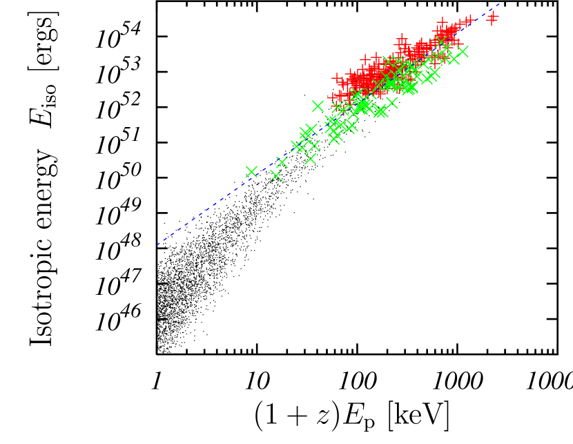
Figure 2: Distribution of simulated bursts in the $(1+z)E_{\rm p}$–$E_{\rm iso}$ plane. Pluses ($+$) and crosses ($\times$) represent bursts that can be detected by HETE-2; the former is on-axis events ($\theta_{v}<\Delta\theta$) while the latter is the off-axis case ($\theta_{v}>\Delta\theta$). The events denoted by dots are not detected. The dashed line represents the best fit of the observation given by $E_{\rm p}\sim 95\,{\rm keV}\,(E_{\rm iso}/10^{52}\,{\rm ergs})^{1/2}$ (Lamb et al., 2003b).

Figure 2 shows a result. Among $10^{4}$ simulated events, 288 events are detected by HETE-2. The others cannot be observed because their viewing angles are so large that the relativistic beaming effect reduces their observed flux below the limiting sensitivity. Pluses ($+$) and crosses ($\times$) represent bursts detected by HETE-2; the former corresponds to on-axis events ($\theta_{v}<\Delta\theta$) while the latter correspond to off-axis events ($\theta_{v}>\Delta\theta$). The events denoted by dots are not detected. The numbers of on-axis and off-axis events are 209 and 79, respectively. Nearby events ($z\lesssim 1$) with large viewing angles can be seen. Such bursts are mainly soft events with $(1+z)E_{\rm p}$ less than $\sim 60$ keV.

When $\theta_{v}<\Delta\theta$, $E_{\rm p}$ is related to $E_{\rm iso}$ as $E_{\rm p}\propto E_{\rm iso}^{1/2}$ [see equation (4)]. The dispersion of pluses ($+$) in the $E_{\rm p}$–$E_{\rm iso}$ plane comes mainly from those of “intrinsic” quantities such as $E_{\gamma}{|_{z=0}^{\theta_{v}=0}}$, $\Delta\theta$ and $\xi$.

On the other hand, even when $\theta_{v}>\Delta\theta$, the relation $E_{\rm p}\propto E_{\rm iso}^{1/2}$ is nearly satisfied for the observed sources. The reason is as follows. For a certain source, as the viewing angle increases, the relativistic beaming and Doppler effects reduce the observed fluence and peak energy, respectively. When the point source approximation is appropriate for the large-$\theta_{v}$ case, the isotropic energy and the peak energy depend on the Doppler factor $\delta=[\gamma(1-\beta\cos(\theta_{v}-\Delta\theta))]^{-1}$ as $E_{\rm iso}\propto S(20-2000~{}{\rm keV})\propto\delta^{1-{\langle\alpha\rangle}}$ and $E_{\rm p}\propto\delta$, respectively (Ioka & Nakamura, 2001; Yamazaki, Ioka, & Nakamura, 2002; Dar & De Rújula, 2003). Hence we obtain $E_{\rm iso}\propto E_{\rm p}^{1-{\langle\alpha\rangle}}$. Here ${\langle\alpha\rangle}$ is the mean photon index in the 20–2000 keV band, which ranges between $\beta_{B}$ and $\alpha_{B}$. Therefore we can explain the relation $E_{\rm p}\propto E_{\rm iso}^{1/2}$ for ${\langle\alpha\rangle}\sim\alpha_{B}\sim-1$. On the other hand, when $\theta_{v}$ is large enough for $E_{\rm p}$ to be smaller than 20 keV, we find $E_{\rm iso}\propto E_{\rm p}^{1-\beta_{B}}\sim E_{\rm p}^{3.3}$ or $E_{\rm p}\propto E_{\rm iso}^{0.3}$ since ${\langle\alpha\rangle}\sim\beta_{B}$. In this case, the relation deviates from the line $E_{\rm p}\propto E_{\rm iso}^{1/2}$, and the dispersion of $E_{\rm iso}$ becomes large for small $E_{\rm p}$.

5 Discussion

We have shown that our simple jet model does not contradict the observed $E_{\rm p}$–$E_{\rm iso}$ relation and extends it to lower $E_{\rm p}$ or $E_{\rm iso}$ values. The low-isotropic energy part of the relation is dominated by off-axis events. The number of off-axis events is about one-third of on-axis emissions. An important prediction of our model has been also derived, i.e., we will see the deviation from the present relation $E_{\rm p}\propto E_{\rm iso}^{1/2}$ if the statistics of the low-energy bursts increase.

HETE team gives definitions of the XRF and the XR-GRB in terms of the hardness ratio: XRFs and XR-GRBs are events for which $\log[S_{X}(2-30~{}{\rm keV})/S_{\gamma}(30-400~{}{\rm keV})]>0.0$ and $-0.5$, respectively (Lamb et al., 2003b; Sakamoto et al., 2003). We calculate the hardness ratio for simulated bursts surviving the fluence truncation condition, and classify them into GRBs, XR-GRBs, and XRFs. It is then found that all XRFs have redshift smaller than 5. The ratio of the observed event rate becomes $R_{GRB}:R_{XR-GRB}:R_{XRF}\sim 2:6:1$. This ratio mainly depends on the value of $q$. When $q$ becomes small, jets with large $\Delta\theta$ increases, and hence intrinsically dim bursts (i.e., low-$E_{\rm iso}{|_{z=0}^{\theta_{v}=0}}$ bursts) are enhanced. Owing to equation (4), soft events are enhanced. In the case of $q=1$ with the other parameters remaining fiducial values, the ratio is $R_{GRB}:R_{XR-GRB}:R_{XRF}\sim 1:9:3$. For any cases we have done, the number of XR-GRBs is larger than those of GRBs and XRFs, while the event rate is essentially comparable with each other. HETE-2 observation shows $R_{GRB}:R_{XR-GRB}:R_{XRF}\sim 1:1:1$ (Lamb et al., 2003b). Although possible instrumental biases may change the observed ratio (Suzuki, M. & Kawai, N., 2003, private communication), we need more studies in order to bridge a small gap between the theoretical and the observational results.

We briefly comment on how the results obtained in this Letter will depend on the Lorentz factor of the jet $\gamma$. If we fix $\gamma=200$, the relativistic beaming effect becomes stronger and less off-axis events are observed than in the case of $\gamma=100$; off-axis events are 13 % of the whole observed bursts when $\gamma=200$, while 27 % for $\gamma=100$. The ratio of the observed event rate for $\gamma=200$ is $R_{GRB}:R_{XR-GRB}:R_{XRF}\sim 2:5:1$, which is similar to that for $\gamma=100$.

The $E_{\rm p}$–$E_{\rm iso}$ diagram of the GRB population may be a counterpart of the Herzsprung-Russell diagram of the stellar evolution. The main-sequence stars cluster around a single curve which is a one-parameter family of the stellar mass. This suggests that the $E_{\rm p}$–$E_{\rm iso}$ relation of the GRB implies the existence of a certain parameter that controls the GRB nature like the stellar mass. We have shown that the viewing angle is one main factor to explain the $E_{\rm p}$–$E_{\rm iso}$ relation kinematically. Our model predicts the deviation of this relation in the small $E_{\rm iso}$ region, which may be confirmed in future.

In the uniform jet model, the afterglows of off-axis jets may resemble the orphan afterglows that initially have a rising light curve (e.g., Yamazaki, Ioka, & Nakamura, 2003a; Granot et al., 2002; Totani & Panaitescu, 2002). The observed $R$-band light curve of the afterglow of XRF 030723 may support our model (Fynbo et al., 2004).

Figure 1: Photon index in the energy range 2–25 keV as a function of the peak flux in the same energy range by varying the source redshift $z$. This figure is the updated version of Fig. 3 in Yamazaki, Ioka, & Nakamura (2002). We adopt $\gamma\Delta\theta=10$, $\alpha_{B}=-1$, $\beta_{B}=-2.5$, and $\gamma\nu^{\prime}_{0}=300$ keV. The values of the viewing angle $\gamma\theta_{v}$ are given in parenthesis. Three solid curves correspond to $z=0.01$, 0.1, and 1, respectively. The same values of $\gamma\theta_{v}$ with different $z$ are connected by dotted lines. The observed data of BeppoSAX-XRFs are shown from Heise et al. (2001). Squares (triangles) are those which were (were not) detected by BATSE. Two dashed lines represent observational bounds. Note that an operational definition of the XRF detected by Wide Field Cameras (WFCs) on BeppoSAX is a fast X-ray transient that is not triggered and not detected by the Gamma-Ray Burst Monitor (GRBM) (Heise et al., 2001). In the region to the left of the vertical dashed line, the peak flux in the X-ray band is smaller than the limiting sensitivity of WFCs, and such events cannot be observed. In the region to the right of the oblique dashed line, the peak flux in the $\gamma$-ray band is larger than the limiting sensitivity of the GRBM, and such events are observed as GRBs.

References

- Amati et al. (2002) Amati, L. et al. 2002, A&A, 390, 81
- Arefiev, Priedhorsky, & Borozdin (2003) Arefiev, V. A., Priedhorsky, W. C., & Borozdin, K. N. 2003, ApJ, 586, 1238
- Atteia (2003) Atteia, J.-L. 2003, A&A, 407, L1
- Band et al. (1993) Band, D. et al. 1993, ApJ, 413, 281
- Band (2003) Band, D.L., 2003, ApJ, 588, 945
- Barraud et al. (2003) Barraud, C. et al. 2003, A&A, 400, 1021
- Bloom, Frail, & Kulkarni (2003a) Bloom, J. S., Frail, D. A., & Kulkarni, S. R. 2003a, ApJ, 594, 674
- Bloom et al. (2003b) Bloom, J. S., Fox, D., van Dokkum, P. G., Kulkarni, S. R., Berger, E., Djorgovski, S. G., & Frail, D. A. 2003b, ApJ, 599, 957
- Daigne & Mochkovitch (2003) Daigne, F. & Mochkovitch, R. 2003, MNRAS, 342, 587
- Dar & De Rújula (2003) Dar, A. & De Rújula, A. 2003, astro-ph/0309294
- Dermer et al. (1999) Dermer, C. D., Chiang, J., & Böttcher, M. 1999, ApJ, 513, 656
- Dermer & Mitman (2003) Dermer, C. D. & Mitman, K. E. 2003, in proc. of Third Rome Workshop: Gamma-Ray Bursts in the Afterglow Era. (astro-ph/0301340)
- Drenkhahn & Spruit (2002) Drenkhahn, G. & Spruit, H. C. 2002, A&A, 391, 1141
- Frail et al. (2001) Frail, D. A. et al. 2001, ApJ, 562, L55
- Fynbo et al. (2004) Fynbo, J. P. U. et al. 2004, astro-ph/0402240
- Gotthelf et al. (1996) Gotthelf, E. V., Hamilton, T. T., & Helfand, D. J. 1996, ApJ, 466, 779
- Granot et al. (2002) Granot, J., Panaitescu, A., Kumar, P., & Woosley, S. E. 2002, ApJ, 570, L61
- Hamilton et al. (1996) Hamilton, T. T., Gotthelf, E. V., & Helfand, D. J. 1996, ApJ, 466, 795
- Heise et al. (2001) Heise, J., in ’t Zand, J., Kippen, R. M., & Woods, P. M. 2001, in Proc. Second Rome Workshop: Gamma-Ray Bursts in the Afterglow Era, ed. E. Costa, F. Frontera, & J. Hjorth (Berlin: Springer), 16 (astro-ph/0111246)
- Heise (2002) Heise, J. 2002, talk given in Third Rome Workshop: Gamma-Ray Bursts in the Afterglow Era.
- Huang, Dai, & Lu (2002) Huang, Y. F., Dai, Z. G., & Lu, T. 2002, MNRAS, 332, 735
- Ioka & Nakamura (2001) Ioka, K., & Nakamura, T. 2001, ApJ, 554, L163
- Ioka & Nakamura (2002) Ioka, K., & Nakamura, T. 2002, ApJ, 570, L21
- Lamb, Donaghy, & Graziani (2003a) Lamb, D. Q., Donaghy, T. Q., & Graziani, C. 2003a, astro-ph/0312634
- Lamb et al. (2003b) Lamb, D.Q. et al. 2003b, astro-ph/0309462
- Mészáros et al. (2002) Mészáros, P., Ramirez-Ruiz, E., Rees, M. J., & Zhang, B. 2002, ApJ, 578, 812
- Mochkovitch et al. (2003) Mochkovitch, R., Daigne, F., Barraud, C., & Atteia, J. 2003, astro-ph/0303289
- Panaitescu & Kumar (2002) Panaitescu, A. & Kumar, P. 2002, ApJ, 571, 779
- Porciani & Madau (2001) Porciani, C. & Madau, P. 2001, ApJ, 548, 522
- Preece et al. (2000) Preece, R. D., Briggs, M. S., Mallozzi, R. S., Pendleton, G. N., Paciesas, W. S., & Band, D. L. 2000, ApJS, 126, 19
- Ramirez-Ruiz & Lloyd-Ronning (2002) Ramirez-Ruiz, E. & Lloyd-Ronning, N. M. 2002, New Astronomy, 7, 197
- Sakamoto et al. (2003) Sakamoto, T., et al. 2003, ApJ, in press (astro-ph/0309455)
- Salmonson & Galama (2002) Salmonson, J. D. & Galama, T. J. 2002, ApJ, 569, 682
- Soderberg et al. (2003) Soderberg, A. M., et al. 2003, submitted to ApJ (astro-ph/0311050)
- Strohmayer et al. (1998) Strohmayer, T. E., Fenimore, E. E., Murakami, T., & Yoshida, A. 1998, ApJ, 500, 873
- Totani & Panaitescu (2002) Totani, T., & Panaitescu, A. 2002, ApJ, 576, 120
- Yamazaki, Ioka, & Nakamura (2002) Yamazaki, R., Ioka, K., & Nakamura, T. 2002, ApJ, 571, L31
- Yamazaki, Ioka, & Nakamura (2003a) Yamazaki, R., Ioka, K., & Nakamura, T. 2003a, ApJ, 591, 283
- Yamazaki, Ioka, & Nakamura (2003b) Yamazaki, R., Ioka, K., & Nakamura, T. 2003b, ApJ, 593, 941
- Yamazaki, Yonetoku, & Nakamura (2003) Yamazaki, R., Yonetoku, D., & Nakamura, T. 2003, ApJ, 594, L79
- Yonetoku et al. (2003) Yonetoku, D., et al. 2003, ApJ in press (astro-ph/0309217)
- Zhang & Mészáros (2002b) Zhang, B. & Mészáros, P. 2002b, ApJ, 581, 1236
- Zhang & Mészáros (2003) Zhang, B. & Mészáros, P. 2003, astro-ph/0311190
- Zhang, Woosley, & Heger (2003) Zhang, W., Woosley, S. E., & Heger, A. 2003, astro-ph/0308389