S-Z Anisotropy & Cluster Counts: Consistent
Selection of $\sigma_{8}$ & the Temperature-Mass Relation

Abstract

The strong dependence of the mass variance parameter, $\sigma_{8}$, on the adopted cluster mass-temperature relation is explored. A recently compiled X-ray cluster catalog and various mass-temperature relations are used to derive the corresponding values of $\sigma_{8}$. Calculations of the power spectrum of the CMB anisotropy induced by the Sunyaev-Zeldovich effect and cluster number counts are carried out in order to assess the need for a consistent choice of the mass-temperature scaling and the parameter $\sigma_{8}$. We find that the consequences of inconsistent choice of the mass-temperature relation and $\sigma_{8}$ could be quite substantial, including a considerable mis-estimation of the magnitude of the power spectrum and cluster number counts. Our results can partly explain the large scatter between published estimates of the power spectrum and number counts. We also show that the range of values of the power-law index in the scaling $C_{\ell}\sim\sigma_{8}^{6-7}$ deduced in previous studies is likely overestimated; we obtain a more moderate dependence, $C_{\ell}\sim\sigma_{8}^{4}$.

and

1 Introduction

Calculations of the power spectrum of CMB anisotropy induced by the Sunyaev-Zeldovich (S-Z) effect, and of cluster number counts, involve various intrinsic cluster quantities, as well as cosmological and cluster mass function parameters. Specifically, the level of S-Z signal in a cluster is directly related to the intracluster (IC) gas temperature and density distributions. The cosmological and large scale structure parameters enter in the expression for the collective mass function of clusters. Most commonly, this function is assumed to have the Press & Schechter (1974) form, but other, more physically established mass functions, are also widely adopted. The mass function is usually normalized by specifying an observationally deduced value of $\sigma_{8}$, the rms density fluctuation on a scale of $8\,h^{-1}$ Mpc. The value of $\sigma_{8}$ may be deduced in several different ways, perhaps most directly from a comparison between the observed two-point correlation function of galaxies or clusters of galaxies, and the spectrum of the primordial density fluctuation field on the relevant scales, recently employed in the analysis of the large SDSS sample (e.g. , Tegmark et al.  2003). Measurements of CMB anisotropy yield a globally averaged value of $\sigma_{8}$, most recently deduced from the first year WMAP measurements (Bennett et al., 2003). Additionally, $\sigma_{8}$ has been deduced from fitting X-ray cluster data (luminosity or temperature functions) to the corresponding theoretical models, with the latter derived from a mass function upon assuming a specific mass-luminosity or mass-temperature relation.

Deduced values of $\sigma_{8}$ clearly depend on data quality, modeling, and analysis methods, as is reflected in the current wide range, $0.5\lesssim\sigma_{8}\lesssim 1.2$. Joint analysis of the SDSS and WMAP databases yields the current ‘best’ (with 6 free ‘vanilla’ parameters) value, $\sigma_{8}=0.917^{+0.090}_{-0.072}$ (Tegmark et al. 2003). This is roughly in agreement (e.g., Wu 2001) or somewhat lower (Viana & Liddle 1999) than results from X-ray cluster studies. The wide range of values of $\sigma_{8}$ has significant implications on the level of various cosmological quantities. Here we explore some of its consequences for the abundance of clusters, and in particular the power of S-Z anisotropy and cluster number counts, quantities that depend steeply on $\sigma_{8}$. Since we concentrate here on clusters, the emphasis will be on values of $\sigma_{8}$ deduced from cluster X-ray measurements, particularly of gas temperatures. Pertinent key features of such analyses are properties of the cluster sample (e.g. , completeness, temperature and redshift ranges), the adopted mass function model, and the mass-temperature relation used to convert the mass function into a temperature function. By comparing the latter function to the observed temperature function, $\sigma_{8}$ (and other parameters, such as $\Omega_{m}$) can be determined.

In this paper we focus on consequences of the choice of the temperature-mass (TM) relation on $\sigma_{8}$, and their impact on the predicted S-Z angular power spectrum and cluster number counts. A quantitative assessment is given of the impact of inconsistent choice of the TM relation and $\sigma_{8}$ on the predicted levels of the the S-Z anisotropy and the number of clusters to be observed by the Planck satellite. Our main goal here is to improve some of the technical aspects in the calculations of these quantities, and to partly explain the large variance among previous estimates of the S-Z power spectrum.

The paper is arranged as follows: the need for a consistent choice of $\sigma_{8}$ and the TM relation, the method employed to extract $\sigma_{8}$ from the observed temperature function, and the variation of $\sigma_{8}$ with the choice of the TM relation are described in § 2. The importance of consistent choice is addressed once more in § 3 and § 4, where its consequences on the S-Z angular power spectrum and cluster number counts are quantified and further elaborated upon in § 5.

2 TM-$\sigma_{8}$ Relation

2.1 Method

The calculation of the S-Z power spectrum involves the basic cosmological and large structure parameters, properties of IC gas, and the cluster mass function (MF). Of the various methods that have been used to calculate the S-Z anisotropy, we employ the approach described in Colafrancesco et al.  (1994, 1997), which we have recently updated and generalized (Sadeh & Rephaeli 2003). The calculation will not be described here; full details are given in the latter paper.

In a cluster temperature-mass relation (TMR) the gas temperature is a monotonically increasing function of mass; $T\propto M^{2/3}$ in virial equilibrium. The temperature function may be written in terms of the MF by

$$N(T)\,dT=N[M(T)]\,\frac{dT}{dM}\,dM.$$ (1)

Since at the high mass end the MF is to a good approximation a monotonically increasing function of $\sigma_{8}$, it can be formally shown (Sadeh & Rephaeli 2003) that:

1. TM relations which predict higher (lower) temperatures for a given mass yield lower (higher) $\sigma_{8}$, and therefore, lower (higher) cluster density.

2. Calculations of the S-Z power spectrum employing a specific TMR, and a value of $\sigma_{8}$ different from the one that would have been extracted by adopting this relation, will result in mis-estimation of S-Z power. The power level will be overestimated (underestimated) when, for a given TMR, the adopted value of $\sigma_{8}$ is higher (lower) than the value corresponding to that particular TMR.

We adopt the procedure developed by Pierpaoli et al. (2001) for the determination of $\sigma_{8}$ from an observationally based temperature function. Given a list of X-ray cluster temperatures and their corresponding redshifts, the temperature function can be deduced. The theoretical MF – with $\sigma_{8}$ as the free parameter – is converted into a temperature function given an assumed TM relation. This is calculated at redshift $z=0.057$, the median redshift of the particular X-ray catalog used. The temperature range in the catalog is divided into a large number of bins, and the mean occupation number of clusters in each of these bins is computed by multiplying $n(T)\,dT$ at the bin temperature by the effective volume occupied at this temperature, i.e., the volume of space to which clusters in the bin can be observed, denoted by $V_{i}$ . A large number of mock catalogs is now devised by using the listed temperatures as the mean of a normally distributed variable, and their $1\sigma$ errors as its variance. The temperature bins are now scanned so as to determine whether any of these is occupied by clusters in the mock catalog. Occupation numbers are assigned to each one of the bins. Assuming a Poissonian distribution of the cluster occupation numbers, the probability of finding $N_{i}$ clusters in bin $i$ is estimated using the Poissonian distribution, with $n(T)\,dT\,V_{i}$ interpreted as the distribution mean. Finally, the likelihood function of obtaining the ‘observed’ occupations in all bins simultaneously is constructed, and maximized against $\sigma_{8}$.

2.2 TM Relations

We employ five TM relations found in the literature; three of these have the same functional form, differing only in the temperature normalization for a fiducial cluster at redshift $z=0$ with mass $10^{15}\,h^{-1}\,M_{\odot}$. The five functions are identified here as models 1-5:

Model 1 (Colafrancesco et al 1997):

$$T=5.78\,(1+z)\,\left(\frac{M}{10^{15}\,h^{-1}\,M_{\odot}}\right)^{2/3}\Omega_{0}^{1/3}\left[\frac{\Delta(\Omega_{0},z)}{\Delta(\Omega_{0}=1,z=0)}\right]^{1/3}.$$ (2)

Model 2 (Tomita 2003):

$$T=5.2\,\gamma\,(1+z)\,\left(\frac{M}{10^{15}\,h^{-1}\,M_{\odot}}\right)^{2/3}\Omega_{0}^{1/3}\left[\frac{\rho_{vir}(z)}{18\pi^{2}}\right]^{1/3},$$ (3)

where $\gamma=1.2$.

Model 3 (Henry 2000):

$$T=\frac{7.98\,keV}{\beta_{TM}}\,(1+z)\,\left(\frac{M}{10^{15}\,h^{-1}\,M_{\odot}}\right)^{2/3}\Omega_{0}^{1/3}\left[\frac{\Delta(\Omega_{0},z)}{18\pi^{2}}\right]^{1/3},$$ (4)

where $\beta_{TM}=1.21$.

Model 4 (Pierpaoli et al. 2001):

$$T=\beta\,\left(\frac{M}{10^{15}\,h^{-1}\,M_{\odot}}\right)^{2/3}(\Delta_{c}\,E^{2})^{1/3}\,\left(1-2\frac{\Omega_{\Lambda}(z)}{\Delta_{c}}\right),$$ (5)

where $E^{2}=\Omega_{m}(1+z)^{3}+\Omega_{\Lambda}$.

Model 5 (Molnar & Birkinshaw 2000):

$$T=2.76\,\beta^{-1}\frac{1-\Omega_{0}}{\Omega_{0}^{2/3}}\left(\frac{M}{10^{15}\,h^{-1}\,M_{\odot}}\right)^{2/3}\left[\left(\frac{2\pi}{\sinh{\eta}-\eta}\right)^{2/3}+\frac{n_{p}+3}{5}\right],$$ (6)

where $\beta$ and $n_{p}$ are taken to be $1$ and $-1.4$, respectively, ($n_{p}$ is the ‘effective’ power index on cluster scales), $\eta=\cosh^{-1}\left[\displaystyle\frac{2}{\Omega_{m}(z)-1}\right]$, and $\Omega_{m}(z)=\displaystyle\frac{\Omega_{0}(1+z)}{\Omega_{0}(1+z)+(1-\Omega_{0})}$.

The first three relations may all be written in the form

$$T=\alpha\,(1+z)\,\left(\frac{M}{10^{15}\,h^{-1}\,M_{\odot}}\right)^{2/3}\,\Omega_{0}^{1/3}\,\left[\frac{\Delta_{c}(\Omega_{0},z)}{18\pi^{2}}\right]^{1/3},$$ (7)

where $\alpha=5.78,6.24,6.59$ in models (1),(2), (3), respectively. In a flat universe with $\Lambda=0$, $\alpha$ is equal to the temperature of a local cluster with mass $10^{15}\,h^{-1}\,M_{\odot}$. In the currently fashionable (‘standard’) $\Lambda CDM$ model, substituting $z=0.053$ in the above relations, the temperatures associated with clusters having this mass are $3.43\,keV,3.71\,keV,3.92\,keV,6.19\,keV,8.49\,keV$, respectively.

2.3 Results for $\sigma_{8}$

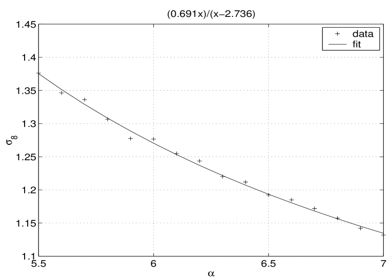
Figure 1: $\sigma_{8}$ as function of the parameter $\alpha$. Each data point represents an average over ten runs. The fitted curve is plotted only for visual purposes.

To verify the validity of the first assertion made in the previous subsection, $\sigma_{8}$ has been estimated using equation 7 with $5.5\leq\alpha\leq 7.0$. For each value of $\alpha$ ten runs were made and average values of $\sigma_{8}$ were computed. A more statistically complete analysis would require a much larger number of runs for each value of $\alpha$, but the consistency of the results suggests that this is not needed for our purposes here. The input and output of the runs are tabulated in table 1 and illustrated in figure 1. It is clear from the plot that (as expected) $\sigma_{8}$ is quite sensitive to the choice of the TM relation. In fact, a relative variance of $\sim 30\%$ in the temperature scaling – which is in accord with typical observational uncertainties – induces a relative change of $\sim 20\%$ in the value of $\sigma_{8}$. This has important practical consequences given that the mass function is extremely sensitive to this parameter. Moreover, these results are in accordance with the qualitative argument summarized above: A TM relation which associates a higher temperature with a given mass yields a lower value of $\sigma_{8}$, and vice versa. The calculated five values of $\sigma_{8}$ are $1.32,\,1.23,\,1.18,\,1.00,\,0.68$, for models 1-5, respectively.

T (keV)	5.5	5.6	5.7	5.8	5.9	6.0	6.1	6.2	6.3	6.4	6.5	6.6	6.7	6.8	6.9	7.0
1	1.366	1.335	1.325	1.325	1.263	1.284	1.253	1.222	1.212	1.232	1.181	1.181	1.181	1.150	1.161	1.150
2	1.386	1.345	1.325	1.294	1.284	1.294	1.273	1.222	1.232	1.222	1.161	1.191	1.181	1.150	1.150	1.130
3	1.386	1.366	1.345	1.325	1.284	1.284	1.243	1.253	1.222	1.232	1.202	1.181	1.171	1.140	1.140	1.130
4	1.397	1.345	1.366	1.325	1.294	1.294	1.253	1.253	1.222	1.222	1.202	1.202	1.181	1.171	1.140	1.120
5	1.386	1.325	1.345	1.285	1.294	1.263	1.273	1.243	1.222	1.212	1.181	1.181	1.181	1.140	1.130	1.130
6	1.345	1.356	1.294	1.315	1.263	1.253	1.232	1.232	1.212	1.202	1.181	1.181	1.161	1.190	1.120	1.130
7	1.376	1.366	1.335	1.294	1.273	1.284	1.243	1.253	1.212	1.202	1.212	1.181	1.161	1.161	1.161	1.140
8	1.356	1.314	1.325	1.315	1.304	1.273	1.253	1.243	1.212	1.222	1.191	1.191	1.191	1.150	1.150	1.140
9	1.366	1.366	1.356	1.284	1.263	1.294	1.253	1.263	1.212	1.202	1.191	1.181	1.161	1.161	1.150	1.130
10	1.397	1.345	1.345	1.304	1.253	1.243	1.273	1.253	1.243	1.170	1.222	1.181	1.151	1.161	1.120	1.120
$<\sigma_{8}>$	1.376	1.346	1.336	1.307	1.278	1.277	1.255	1.244	1.220	1.212	1.192	1.185	1.172	1.157	1.142	1.132

Table 1: Values of $<\sigma_{8}>$ for the adopted TM relation

3 Dependence of the Power Spectrum on $\sigma_{8}$ and the TMR

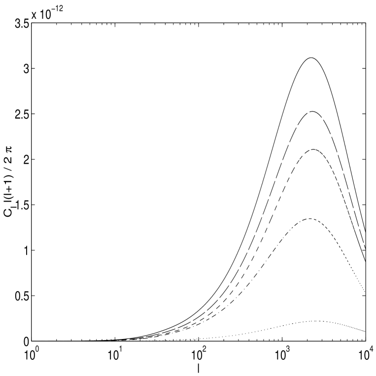
Figure 2: The angular power spectrum of the S-Z effect calculated using the five M-T relations of models 1-5, and their matching $\sigma_{8}$s as presented in § 3. Solid, long dashed, short dashed, dashed-dotted and dotted curves correspond to models 1,2,3,4 and 5, respectively.

The S-Z power spectrum was calculated (Sadeh & Rephaeli 2003) employing the five models described above. We first calculated the power for each of the five TM relations and its matching $\sigma_{8}$, and then crossed these inputs by taking the TM relation of model $i$ and $\sigma_{8}$ corresponding to model $j$, where $i\neq j=1-5$. Results of the first calculations are shown in figure 2; these reflect the tight relation between the magnitude of the power spectrum and the cluster population. Note that although lower temperatures (implied by a ‘colder’ TM calibration) will tend to reduce the power, the influence of the higher $\sigma_{8}$ dominates, resulting in a higher level of power.

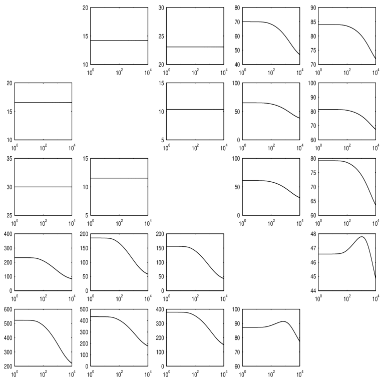
Figure 4: As in figure (3), but here the relative differences between the dashed and dash-dotted curves (i.e., consistent vs. inconsistent calculations) are specified in percentage units.

The results of the second set of ‘cross’ calculations are described in figure 3. Each panel contains three curves; the solid curves represent calculations employing a specific TMR and its corresponding $\sigma_{8}$. The dash-dotted curves show results of the calculations employing the same TMR as for the solid curves, but a different $\sigma_{8}$. Finally, the dashed curves show results for the same $\sigma_{8}$ as in the dash-dotted curves, but with the TMR that corresponds to this parameter, thereby providing a ‘correction’ to the results illustrated by the dash-dotted curves. In order to further clarify the results, the first row will be considered as an example: In the first panel (2nd from the left) the TMR of model 1 is used; here the temperatures are lowest, and $\sigma_{8}$ assumes the highest value; the solid curve describes this case. Now $\sigma_{8}$ is changed to the value extracted using model 2, i.e., a lower value. However, in combination with the TMR of model 1, the power spectrum is underestimated, since the TMR of model 2 should have been used, rather than that of model 1. Indeed, model 2 predicts higher temperatures than model 1, and therefore the correct power spectrum is represented by the dashed curve. Obviously, as the difference between the correct $\sigma_{8}$ and the one employed in the calculation increases, the degree of underestimation (or overestimation) also increases, as can be seen in the next panels of the first row. The relative errors introduced by the inconsistent choice of these two elements can be readily calculated; this is presented in figure 4. As anticipated, the panels lying on both sides of the diagonal show lower relative errors than those located further away from the diagonal, where differences between adopted and correct values of $\sigma_{8}$ are larger. Errors of up to a factor of $\sim 5$ are caused by this parameter mismatch. The relative errors among the first three models are constant along the multipole axis due to their functional uniformity. In other cases the relative error changes with $\ell$.

The dependence of the S-Z power on $\sigma_{8}$ has already been discussed in previous works, it is usually demonstrated by arbitrarily changing its value. Although the change is not great (as the ones required in order to induce a relative error of hundreds of percents as seen in figure 4), a difference of $\lesssim 20\%$ (e.g. $\sigma_{8}=0.9-1.1$) or more is common. Examples for large errors induced by a change of $\sim 18\%$ in $\sigma_{8}$ may be seen in the third panels of the third and fourth rows of figure 4: in the third row the correct and unmatched values of $\sigma_{8}$ are $1.18$ and $1.0$, respectively, and a relative error of $\sim 40-50\%$ appears around $\ell=1000$. In the fourth row the correct and unmatched values are $1.0$ and $1.18$, respectively, and a relative error of $>50\%$ is induced.

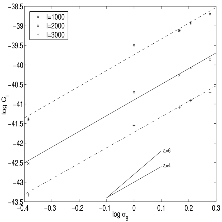
Figure 5: The dependence of $C_{\ell}$ on $\sigma_{8}$, illustrated in a Log-Log plot. Asterices, x-marks and plus symbols represent $C_{\ell}$s at five different $\sigma_{8}$s, corresponding to models 1-5, for $\ell=1000,2000,3000$. The dashed, solid, and dash-dotted curves depict the best linear fits for each of the 5 data point sets. The two short lines appearing at the bottom of the plot are of slopes 4 and 6, as indicated in the figure.

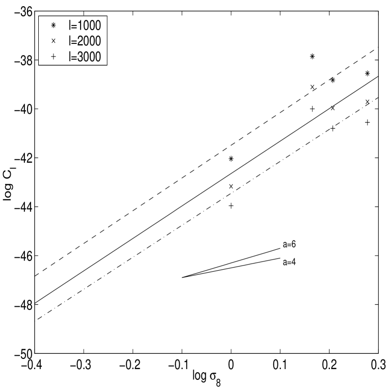
Figure 6: The same as figure (5), but here the TMR models 2-5 are used in conjunction with non-matching $\sigma_{8}$s, extracted from models 1-4, respectively. Thus, both higher values of $\sigma_{8}$ and temperatures scaled from the TMR are used, leading to an overestimation of the power spectrum.

The steep dependence of the S-Z power on $\sigma_{8}$ was quantified by the proportionality $C_{\ell}\propto\sigma_{8}^{6-7}$ (e.g., Komatsu & Tetsu 1999). Our results indicate that this dependence is somewhat more moderate, which is to be expected since an increase of $\sigma_{8}$ implies a decrease in temperature by virtue of the anti-correlation between these two parameters, as has been shown above and illustrated in figure (1). For the three representative value of the multipole (marking the range in which the peak of the S-Z power spectrum occurs) $\ell=1000,\,2000,\,3000$, we plotted the corresponding $C_{\ell}$s in models 1-5 against their corresponding $\sigma_{8}$. Best fits describing the three sets of five data points all have slopes $\sim 4$, smaller than the values ($\sim 6-7$) previously reported. This is illustrated in figure (5). For comparison, we include figure (6), in which the same analysis is applied, but here the TMR models 2-5 are used in conjunction with the $\sigma_{8}$s extracted using models 1-4. The corresponding power spectra are represented by the dash-dotted curves in the four panels under the central diagonal of figure (3). Recall that the resulting power spectrum in this case is overestimated due to the fact that the TMR used in its evaluation would necessitate a lower $\sigma_{8}$ than the one used in the calculation. Thus, a steeper slope is expected in the $\log{C_{\ell}}-\log{\sigma_{8}}$ plot, which is indeed the case. The resulting slopes are actually steeper ($\sim 13$) than $a\approx 6-7$, but the essential result of this analysis is that the scaling $C_{\ell}-\sigma_{8}$ is indeed sensitive to the adopted TMR and its normalization.

4 Dependence of Cluster Counts on $\sigma_{8}$ and the TMR

As is well known, the fact that the S-Z effect is independent of redshift makes it an (almost) ideal tool for the detection of distant clusters. Cluster surveys are planned by several S-Z projects, culminating (according to current plans) with the full sky mapping by the PLANCK satellite. The 143 GHz and 353 GHz channels of the HFI experiment on PLANCK are particularly suitable for detecting large numbers of clusters. The S-Z flux from a cluster is given by (e.g. Colafrancesco et al. 1997)

$$\Delta F_{\nu}(\gamma_{\ell})=\int R_{s}(|\hat{\gamma}-\hat{\gamma_{\ell}}|,\sigma_{B})\,\Delta I_{\nu}(\hat{\gamma})\,d\Omega,$$ (8)

where $\Delta I_{\nu}$ is the change of the CMB spectral intensity due to the thermal component of the S-Z effect. In the non-relativistic limit, $\Delta I_{\nu}=g(x)=x^{4}e^{x}(e^{x}-1)^{-2}\left[x\coth(x/2)-4\right]$, where $T_{0}$ is the CMB temperature, and $y$ is the Comptonization parameter integrated along a los. The more accurate expression for $\Delta I_{\nu}$ includes relativistic corrections (Rephaeli 1995, Itoh et al.  1998, Shimon & Rephaeli 2003). Since our main aim here is to display the dependence of cluster number counts on $\sigma_{8}$ and the TMR – rather than precisely predicting the expected number of clusters – we use the simpler non-relativistic limit of $\Delta I_{\nu}$. We can then write for the S-Z flux

$$\Delta F_{\nu}=\displaystyle\frac{2(k_{b}T_{0})^{3}}{(hc)^{2}}g(x)y_{0}\int R_{s}(|\hat{\gamma}-\hat{\gamma_{\ell}}|,\sigma_{B})\cdot\zeta(|\hat{\gamma_{\ell}}|,M,z)\,d\Omega,$$ (9)

where

$$\zeta(|\hat{\gamma_{\ell}}|,M,z)\equiv\displaystyle\frac{1}{\sqrt{1+(\theta/\theta_{c})^{2}}}\cdot\tan^{-1}{\left[p\sqrt{\frac{1-(\theta/p\theta_{c})^{2}}{1+(\theta/\theta_{c})^{2}}}\right]}.$$ (10)

The measured signal is actually weighted over the spectral response of the detector, $E_{\nu}$, usually approximated by a Gaussian, $G_{\nu}$. Therefore,

$$\Delta\overline{F}_{\nu}=\displaystyle\frac{\int\Delta F_{\nu}E(\nu)d\nu}{\int E(\nu)d\nu}.$$ (11)

For simplicity, $G_{\nu}$ is taken here to be uniform over the passband centered on the central frequency. For the PLANCK/HFI $143\,$GHz channel, beam size is $8^{\prime}$ and $\Delta\nu/\nu=0.25$. The predicted number of clusters with flux greater than $\Delta\overline{F}_{\nu}$ can now be calculated using

$$N(\Delta\overline{F}_{\nu})=\int r^{2}\frac{dr}{dz}dz\int_{\Delta\overline{F}_{\nu}}B(M,z)N(M,z)dM.$$ (12)

The lower limit of the mass function integral is such as to correspond to the limiting flux from a cluster with mass $M$, which we take to be $30\,$mJy, the flux limit reachable in a one year observation. To evaluate this limiting mass, a binary function $B(M,z)$ is introduced. $B(M,z)=1$ if the flux corresponding to a given mass (and redshift) is greater than the limiting flux; otherwise, $B(M,z)=0$.

The predicted number of detectable clusters with mass $M$ at redshift $z$ is proportional to the MF evaluated at these parameters. This depends on the integrated Comptonization parameter along all lines of sight to the cluster. Consequently, the arguments presented in § 2 are relevant also in this case. In figure 7 the predicted cumulative number counts in models 1-5 are shown. A strong relation between the MF normalization and the cluster counts is clearly manifested. It may also be inferred from the figure that the largest contribution to the counts comes from clusters lying at redshifts $\lesssim 0.4$. Since the redshift distribution of clusters cannot be determined from S-Z measurements, the most relevant quantity is indeed the cumulative cluster counts at low redshifts. Results of the ‘cross’ calculations are presented in figure 8. The curves in figure 8 resemble those in figure 3 in the sense that the differences between the values represented by the ‘mismatched’ and ‘correct’ curves increase farther away from the diagonal. The relative differences between the properly and improperly calculated numbers span a range of $\sim 10-70\%$ at the lowest redshifts, corresponding to the maximal cluster counts that would be detected in an all-sky S-Z survey.

Although not observable, the larger differences exhibited at higher redshift reflect the higher sensitivity of the MF to $\sigma_{8}$ at the high-mass end. At such high redshifts only the most massive clusters would be detected, owing to their larger fluxes, and therefore any change in the normalization that does not match the TMR used to evaluate the flux, would result in larger deviations of the counts with respect to a model employing a specific TMR and its corresponding normalization. A comparison between the results illustrated in figures 3 and 8 suggests that an inconsistent choice of $\sigma_{8}$ and the TMR results in a rather pronounced over- or under-estimation of the power spectrum, and a milder (but significant) mis-estimation in the cumulative number counts, in particular at the lowest redshifts. This difference is clearly due to the steeper (gas) temperature dependence of the power ($\propto T_{e}^{2}$) as compared to the corresponding linear dependence of the flux.

5 Conclusion

Predicted profiles and levels of the angular power spectrum of the S-Z effect and of cluster number counts are strongly affected by modeling details and the particular choice of parameter values which explain the large variance in the values of these quantities in the literature. In this paper we focused on the tight dependence between the TMR and $\sigma_{8}$. We demonstrated that selecting these independently is generally not self-consistent and leads to considerable mis-estimation of the power spectrum and cluster counts. This can be is avoided when $\sigma_{8}$ is determined from CMB and large scale structure surveys that do not involve cluster TMRs.

Acknowledgement: This research has been supported by the Israeli Science Foundation grant 729$\backslash$00-03 at Tel-Aviv University.

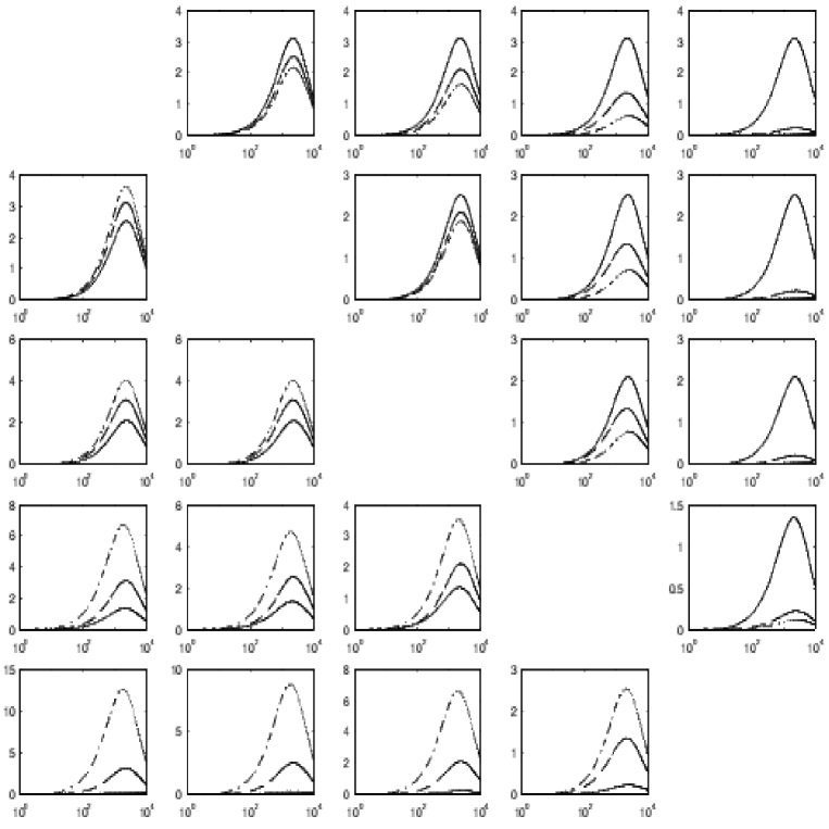
Figure 3: The S-Z power spectrum calculated using unmatched TM relations and $\sigma_{8}$ normalization. Units of the abscissa and ordinate are $\ell$ and $10^{-12}\,\ell(\ell+1)\,C_{\ell}/2\pi$, respectively. Rows 1-5 correspond to models 1,2,3,4,5. Columns 1-5 correspond to the correct $\sigma_{8}$ for the model. Solid curves depict the ‘diagonal’ terms, that is, calculations carried out with a specific TMR and its corresponding $\sigma_{8}$. Dash-dotted curves describe calculations made with the same TMR, but unmatched $\sigma_{8}$. Finally, the dashed curves illustrate the ‘corrected’ power spectrum, i.e. keeping the unmatched $\sigma_{8}$ but now using the matching TMR.

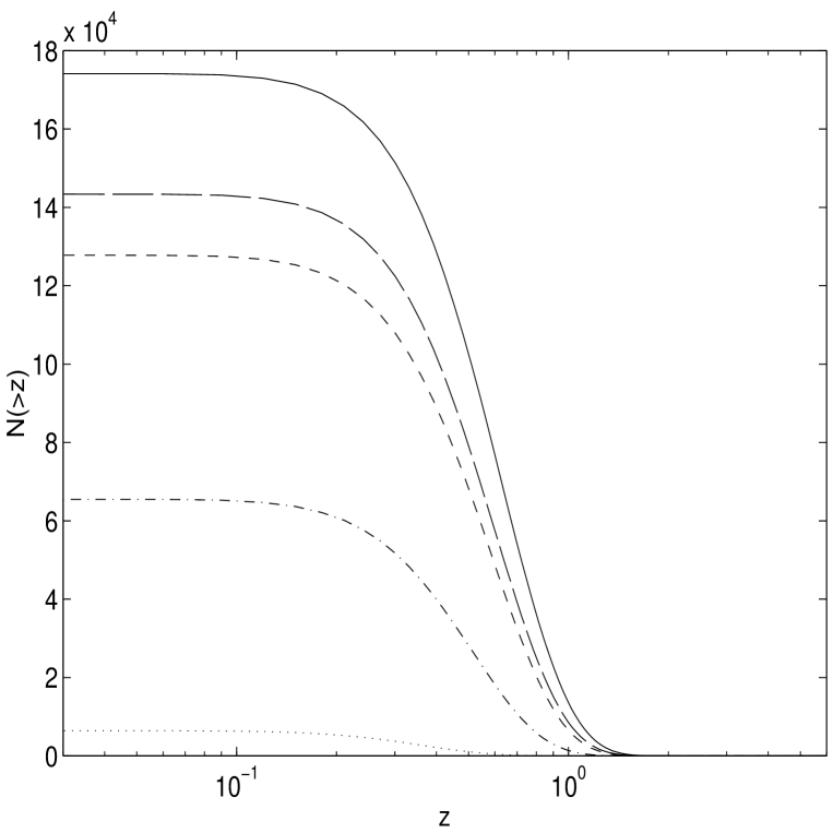
Figure 7: S-Z cluster number counts calculated using the five TMR described above, and their matching values of $\sigma_{8}$. As in figure (2), solid, long dashed, short dashed, dash-dotted and dotted curves correspond to models 1,2,3,4 and 5, respectively.

Figure 8: Cluster number counts calculated using unmatching M-T relations and normalizations, in likeness with figure (3). Abscissa and ordinate units are redshifts and counts.

References

- [1]
- [2] [] Bennett et al. 2003, (astro-ph/0302207)
- [3] [] Colafrancesco S., Mazzotta P., Rephaeli Y., & Vittorio N., 1994, Ap. J. , 433, 454 (1994ApJ...433..454C)
- [4] [] Colafrancesco S., Mazzotta P., Rephaeli Y., & Vittorio N. 1997, Ap. J. , 479, 1 (1997ApJ...479....1C)
- [5] [] Henry J.P., 2000, Ap. J. , 534, 565 (2000ApJ...534..565H)
- [6] [] Itoh N., Kohyama Y., & Nozawa S., 1998, Ap. J. , 502, 7 (1998ApJ...502....7I)
- [7] [] Komatsu E. & Tetsu K., 1999, Ap. J. Lett. , 526, L1-L4 (1999ApJ...526L...1K)
- [8] [] Molnar S.M. & Birkinshaw M. 2000, Ap. J. , 537, 542 (2000ApJ...537..542M)
- [9] [] Pierpaoli E., Scott D., White M., 2001, MNRAS , 325, 77 (2001MNRAS.325...77P)
- [10] [] Press W.H. & Schechter P., 1974, Ap. J. , 187, 425 (1974ApJ...187..425P)
- [11] [] Rephaeli Y., 1995, Annu. Rev. Astron. Astrophys. , 33, 541 (1995ARA&A..33..541R)
- [12] [] Sadeh S. & Rephaeli Y., 2003, New Astronomy , 9, 159
- [13] [] Shimon M. & Rephaeli Y., 2003, New Astronomy , 9, 69
- [14] [] Tegmark M. et al. . Available from astro-ph/0310723
- [15] [] Tomita K. Available from astro-ph/0306154
- [16] [] Viana P.T.P. & Liddle A.R., 1999, MNRAS , 303, 535 (1999MNRAS.303..535V)
- [17] [] Wu J.-H.P., 2001, MNRAS , 327, 629 (2001MNRAS.327..629W)