A Friedmann-Lemaître-Robertson-Walker cosmological model with running $\Lambda$

Abstract:

The idea of a variable dark energy has been entertained many times in the literature and from many different points of view. Quintessence is just a popular way to implement this idea in recent times, but so far with little success. Another possibility is to think of the cosmological term, $\Lambda$, as a “running quantity” much in the same way as the electromagnetic coupling constant. However, the fact that $\Lambda$ is a dimension-four parameter implies that it may obey a peculiar renormalization group equation, which at low energies could be dominated by “soft decoupling” contributions of the form $\Lambda\sim H^{2}\,M_{P}^{2}\,$ stemming from physics near the Planck scale. This value lies in the ballpark of the measurements from CMB and high-z supernovae. A “renormalized” FLRW cosmology of this kind may reveal itself as a sound, and testable, proposal for a variable $\Lambda$ model within quantum field theory in curved space time.

1 Introduction

The Friedmann-Lemaître-Robertson-Walker (FLRW) cosmological model  [1] constitutes the standard paradigm of present day cosmology. Its 4-curvature is determined from the various contributions to its total energy-momentum tensor density, namely in the form of matter energy density, radiation pressure and cosmological constant:

$$R=8\,\pi\,G_{N}\,(\rho-3\,p+4\,\Lambda)\,.$$ (1)

The cosmological constant contribution to the curvature of space-time is represented by the $\Lambda$ term. The latter enters the original gravitational field equations in the form

$$R_{\mu\nu}-\frac{1}{2}g_{\mu\nu}R=-8\pi G_{N}\ \tilde{T}_{\mu\nu}\,,$$ (2)

where $\tilde{T}_{\mu\nu}$ is given by $\tilde{T}_{\mu\nu}\equiv T_{\mu\nu}+g_{\mu\nu}\,\Lambda(t)$, $T_{\mu\nu}$ being the ordinary energy-momentum tensor associated to isotropic matter and radiation. Here we entertain the possibility that $\Lambda$ is a function of time . By the Bianchi identities, it follows that $\Lambda$ is a constant if and only if the ordinary energy-momentum tensor is individually conserved ($\bigtriangledown^{\mu}\,{T}_{\mu\nu}=0$). In particular, $\Lambda$ must be a constant if ${T}_{\mu\nu}$ is zero (e.g. during inflation).

Modeling the expanding universe as a perfect fluid with velocity $4$-vector field $U^{\mu}$, we have

$$T_{\mu\nu}=-p\,g_{\mu\nu}+(\rho+p)U^{\mu}U^{\nu}\,,$$ (3)

where $p$ is the isotropic pressure and $\rho$ is the proper energy density of matter. Clearly the modified $\tilde{T}_{\mu\nu}$ defined above takes the same form as (3) with $\rho\rightarrow\tilde{\rho}=\rho+\Lambda\,,\ \ \ p\rightarrow\tilde{p}=p-\Lambda$. With this generalized energy-momentum tensor, and in the FLRW metric ($k=0$ for flat, $k=\pm 1$ for spatially curved, universes)

$$ds^{2}=dt^{2}-a^{2}(t)\left(\frac{dr^{2}}{1-k\,r^{2}}+r^{2}\,d\theta^{2}+r^{2}\,\sin^{2}\theta\,d\phi^{2}\right)\,,$$ (4)

the gravitational field equations boil down to the Friedmann-Lemaître equation

$$H^{2}\equiv\left(\frac{\dot{a}}{a}\right)^{2}=\frac{8\pi\,G_{N}}{3}\left(\rho+\Lambda\right)-\frac{k}{a^{2}}\,,$$ (5)

and the dynamical field equation for the scale factor:

$$\ddot{a}=-\frac{4\pi}{3}G_{N}\,(\tilde{\rho}+3\,\tilde{p})\,a=-\frac{4\pi}{3}G_{N}\,(\rho+3\,p-2\,\Lambda)\,a\,.$$ (6)

The physical CC is the parameter $\Lambda$ involved in the equations (5) and (6). As these equations are used to fit the cosmological data [2, 3], the parameter $\Lambda$ involved in them is to be considered the physical (observed) value of the cosmological constant. A first integral of the system (5) and (6) is given by

$$\dot{\Lambda}+\dot{\rho}+3\,H\,(\rho+p)=0\,,$$ (7)

which shows that a time-variable CC cosmology allows transfer of energy from matter-radiation into vacuum energy, and vice versa. Since the radiation pressure is negligible at present, Eq. (5) can be rewritten as the following exact sum rule for the cosmological parameters:

$$\Omega_{M}^{0}+\Omega_{\Lambda}^{0}+\Omega_{K}^{0}=1\,,$$ (8)

with

$$\Omega_{M}^{0}\equiv\frac{\rho_{M}^{0}}{\rho_{c}^{0}}\,,\ \ \ \Omega_{\Lambda}^{0}\equiv\frac{\Lambda_{0}}{\rho_{c}^{0}}\,,\ \ \ \Omega_{K}^{0}\equiv\frac{-k}{H_{0}^{2}\,a_{0}^{2}}\,,$$ (9)

$\rho_{M}^{0}$ and $\Lambda_{0}$ being the matter density and cosmological constant at our time, and

$$\rho_{c}^{0}\equiv\frac{3\,H_{0}^{2}}{8\,\pi\,G_{N}}\simeq 10.6\,h_{0}^{2}\ GeV/m^{3}\simeq\left(3.0\,\sqrt{h_{0}}\times 10^{-3}\,eV\right)^{4}$$ (10)

is the present value of the critical density (equivalent to a few protons per cubic meter). Here the dimensionless number $h_{0}\sim 0.7\pm 0.1$ sets the typical range for today’s value of Hubble’s constant $H_{0}\equiv\left(\dot{a}/{a}\right)_{0}=100\;(Km/sec\,Mpc)\;h_{0}$.

What is the nature of the total energy density of the universe? On the one hand the baryonic contribution to the total matter content $\rho_{M}$ (a scanty $\Omega_{B}\sim 5\%$ of the critical density, derived from nucleosynthesis calculations) is far smaller than the total amount of matter detected by dynamical means [1, 4, 5], namely $\Omega_{M}^{0}\sim 30\%$ of the critical density. Therefore the bulk of the matter content of the universe is dark matter, and must be in the form of an unknown kind of cold (non-relativistic and non-baryonic) invisible component. Significant amounts of hot (relativistic) dark matter are excluded because it would not fit with the models of structure formation (particularly at small scales). So the radiation part at present boils down to an insignificant (few per mil) fraction of neutrinos (yet comparable to the total amount of luminous matter that we see!) plus an even more negligible contribution of very soft photons (the relic CMB radiation) entering at the level of one ten-thousandth, at most, of the critical density today [4, 5].

On the other hand, the astrophysical measurements tracing the rate of expansion of the universe with high–z Type Ia supernovae [2, 3] indicate that $\Omega_{\Lambda}^{0}\sim 70\%$ of the critical energy density of the universe is cosmological constant (CC) or a dark energy candidate with a similar dynamical impact on the evolution of the expansion of the universe. Specifically, the CC value found from Type Ia supernovae at high z is:

$$\Lambda_{0}=\Omega_{\Lambda}^{0}\,\rho_{c}^{0}\simeq 6\,h_{0}^{2}\times 10^{-47}\,GeV^{4}\,.$$ (11)

Independent from these supernovae measurements, the CMB anisotropies [4], including the recent data from the WMAP satellite, lead to $\Omega_{0}=1.02\pm 0.02$ [5]. As a first observation, it is obvious that this result leaves little room for our universe to be spatially curved ($\Omega_{K}\leq 2\%$), and indeed it suggests that our universe is spatially flat, as expected from inflation [6]. As a second observation, when combining this result with the dynamically determined value (from clusters of galaxies) of the matter density (viz. $\Omega_{M}^{0}\simeq 30\%$), the bookkeeping in Eq. (8) leads us to an outstanding conclusion: the rest of the present energy budget (a large gap of order $70\%$ of the critical density) must be encoded in the parameter $\Omega_{\Lambda}^{0}$. Hence the CMB measurements and the high-z supernovae data lead to a conclusion in concordance with the value of $\Lambda$, if one accepts the data on $\Omega_{M}^{0}$ from clusters. As mentioned, the value (11) corresponds to the parameter entering the classical cosmological equations (5) and (6). Therefore the situation seems to be consistent from the experimental point of view 

What about the theoretical situation? In Quantum Field Theory (QFT) we have long expected that the vacuum fluctuations should induce a non-vanishing value for $\Lambda$ [8], and the question is whether in realistic QFT’s we have a prediction for $\Lambda_{0}$ in the ballpark of the measured value (11). Sadly, the answer is no. For, in the context of the Standard Model (SM) of electroweak interactions, this measured CC should be the sum of the original vacuum CC in Einstein’s equations, $\Lambda_{vac}$, and the induced contribution from the vacuum energy of the quantum fields:

$$\Lambda=\Lambda_{vac}+\Lambda_{ind}\,.$$ (12)

What is the expected value for $\Lambda_{ind}$ in the SM? Let $\Phi$ be the quantum Higgs field operator. In the ground (vacuum) state of the SM, the vacuum expectation value (VEV) of $\,\Phi^{+}\Phi\,$ will be denoted $\,<\Phi^{+}\Phi>\equiv\frac{1}{2}\phi^{2}$, where $\,\phi\,$ is the mean field associated to the field operator $\Phi$. The classical potential associated to the mean field reads

$$V_{cl}=-\frac{1}{2}m_{\phi}^{2}\phi^{2}+\frac{\lambda}{8}\phi^{4}.$$ (13)

Shifting the original field $\phi\rightarrow H^{0}+v$ such that the physical scalar field $H^{0}$ has zero VEV one obtains the physical mass of the Higgs boson: $M_{H}=\sqrt{2}\;m_{\phi}$. Minimization of the potential (13) yields the spontaneous symmetry-breaking relation:

$$\phi=\sqrt{\frac{2m_{\phi}^{2}}{\lambda}}=v\,\,\,\,\,\,\mathrm{and}\,\,\,\,\,\,\,\lambda=\frac{M_{H}^{2}}{v^{2}}\,.$$ (14)

The VEV $<\Phi>\equiv v/\sqrt{2}$ gives masses to fermions and weak gauge bosons through

$$m_{f_{i}}=h_{i}\,\frac{v}{\sqrt{2}}\,,\;\;\;M_{W}^{2}=\frac{1}{4}\,g^{2}\,v^{2},\;\;\;M_{Z}^{2}=\frac{1}{4}\,(g^{2}\,+g^{\prime 2})\,v^{2},$$ (15)

where $h_{i}$ are the corresponding Yukawa couplings, and $g\,$ and $\,g^{\prime}\,$ are the $SU(2)_{L}$ and $U(1)_{Y}$ gauge couplings. The VEV can be written entirely in terms of the Fermi scale $M_{F}\equiv G_{F}^{-1/2}\simeq 293\,GeV$ as follows: $\,v=2^{-1/4}M_{F}\simeq 246\,GeV$. From (14) one obtains the following value for the potential, at the tree-level, that goes over to the induced CC:

$$\Lambda_{ind}=<V_{cl}>=-\frac{m_{\phi}^{4}}{2\lambda}=-\frac{1}{8}\,M_{H}^{2}\,v^{2}\,.$$ (16)

From the current LEP 200 numerical bound on the Higgs boson mass, $\,M_{H}>114.1\,GeV$ [9], one finds $\,\,\,\left|\Lambda_{ind}\right|>1.0\times 10^{8}\,GeV^{4}$. Clearly, $\left|\Lambda_{ind}\right|$ is $55$ orders of magnitude larger than the observed CC value (11). Moreover, the Higgs potential gets renormalized at higher order in perturbation theory, and therefore it is the value of the effective Higgs potential $V_{\rm eff}$ what matters at the quantum level. These quantum corrections by themselves are already much larger than (11). Finally, we also note that in general the induced term may also get contributions from strong interactions, the so-called quark and gluon vacuum condensates. These are also huge as compared to (11), but are much smaller than the electroweak contribution (16).

Such discrepancy, the so-called “old” cosmological constant problem (CCP) [10, 11], manifests itself in the necessity of enforcing an unnaturally exact fine tuning of the original cosmological term $\Lambda_{vac}$ in the vacuum action that has to cancel the induced counterpart $\,\Lambda_{ind}$ within a precision (in the SM) of one part in $\,10^{55}$. This big conundrum has triggered many theoretical proposals. On the first place there is the longstanding idea of identifying the dark energy component with a dynamical scalar field [12, 13]. More recently this approach took the popular form of a “quintessence” field slow–rolling down its potential [14] and variations thereof [15]. The main advantage of the quintessence models is that they could explain the possibility of an evolving vacuum energy. This may become important in case such evolution will be someday detected in the observations, although it is not obvious that the models can be easily discriminated [16]. Furthermore, a plethora of suggestions came along with string theory developments [17] and anthropic scenarios [18]. Other recent ideas have been put forward, like the intriguing proposal of non-point-like gravitons at sub-millimeter distances [19], or the suggestion of having multiple degenerate vacua [20].

There are however other (less exotic) possibilities, which should be taken into account. In a series of recent papers [21, 22], the idea has been put forward that already in standard QFT it should not make much sense to think of the CC as a constant, even if taken as a parameter at the classical level, because the Renormalization Group (RG) effects may shift away the prescribed value, in particular if the latter is assumed to be zero. Thus, in the RG approach one takes a point of view very different from the quintessence proposal, as we deal all the time with a “true” cosmological term. It is however a variable one, and therefore a time-evolving, or redshift dependent: $\Lambda=\Lambda(z)$. Although we do not have a QFT of gravity where the running of the gravitational and cosmological constants could ultimately be substantiated, a semiclassical description within the well established formalism of QFT in curved space-time (see e.g. [23, 24]) should be a good starting point. Then, by looking at the CCP from the RG point of view  [25], the CC becomes a scaling parameter whose value should be sensitive to the entire energy history of the universe – in a manner not essentially different to, say, the electromagnetic coupling constant.

The canonical form of renormalization group equation (RGE) for the $\Lambda$ term at high energy is well known – see e.g. [24]. However, at low energy decoupling effects of the massive particles may change significantly the structure of this RGE, with important phenomenological consequences. This idea has been elaborated recently by several authors from various interesting points of view [21, 22, 26, 27]. It is not easy to achieve a RG model where the CC runs smoothly without fine tuning at the present epoch. In Ref. [28, 29, 30] a successful attempt in this direction has been made, which is based on the possible existence of physics near the Planck scale. In the following we review the main features and implications of this “RG-cosmology”.

2 Running cosmological constant

It is well known that the effective action of vacuum takes the form [23, 24]:

$$S_{vac}=\int d^{4}x\sqrt{-g}\,\Big{\{}\,a_{1}R^{2}_{\mu\nu\alpha\beta}+a_{2}R^{2}_{\mu\nu}+a_{3}R^{2}+a_{4}{\square}R-\frac{1}{16\pi G_{vac}}\,R-\Lambda_{vac}\Big{\}}\,,$$ (17)

and at low energies the only relevant part for phenomenological considerations is the Hilbert-Einstein piece

$$S_{HE}=-\int d^{4}x\sqrt{-g}\,\left(\,\frac{1}{16\pi G}\,R+\Lambda_{vac}\,\right)\,.$$ (18)

While the phenomenological impact of the higher derivative terms in (17) is negligible at low energy (namely, at current times), the presence of the parameter $\Lambda_{vac}$ is as indispensable as any one of these higher derivative terms to achieve a renormalizable QFT in curved space-time . Admittedly the vacuum CC itself, $\Lambda_{vac}$, is not the physical (observable) value of the cosmological constant. However, its presence is essential to make possible the matching of the theoretical value of $\Lambda$ in Eq. (12) with the physical measurement (11). Here we do not address the issue of why the two terms (induced and vacuum terms) cancel with the desired precision (the “old” CCP). Rather, we take it for granted, and then study the possibility that the cosmological constant evolves according to a RGE whose flow crosses the present instant of time with the value (11), and we then investigate whether such a RGE, when extrapolated back to the past, gives testable and consistent predictions. In particular, we verify whether the predicted value of $\Lambda$ at the nucleosynthesis time does not disturb the basic features of this momentous regime in the history of the universe. Once this is guaranteed, we wish to check whether the predictions of the RGE for nearby past times depart significantly from the standard FLRW cosmology, and therefore whether we can find out signs that can effectively discriminate among the two. Finally, the same RGE can give us a prediction for the future or destiny of our universe.

Of course the first issue is to elucidate the structure of the RGE for the $\Lambda$ term at any given energy regime. A first clue is to recognize that this renormalization group equation is well-know at high energy [24, 21]. For particles $i=1,2,3,...$ of masses $m_{i}$ and spins $J_{i}$ one finds [21]:

$$\frac{d\Lambda}{d\ln\mu} =\frac{1}{(4\pi)^{2}}\,\sum_{i}\,A_{i}\,m_{i}^{4}$$ (19)

where

$$A_{i}=(-1)^{2J_{i}}(J_{i}+1/2)\,n_{J_{i}}\,N_{c}\,,$$ (20)

with $n_{\{0,1,1/2\}}=(1,1,2)$ and $N_{c}=1,3$ for uncolored and colored particles respectively. However, this equation applies only if the masses $m_{i}$ do correspond to active degrees of freedom (d.o.f.), namely if the RG scale $\mu$ satisfies $\mu\gg m_{i}$ for all $i=1,2,3,...$. Any mass that does not satisfy this condition must be dropped from that RGE. At the same time this raises two issues: i) One is the meaning of the RG scale $\mu$ in cosmology, and the other is: ii) what happens with the decoupled contributions, i.e. those heavy masses that satisfy $M_{i}>\mu$ for a given value of the RG scale. This question has been addressed in Ref. [21, 26] where it was first recognized that the contribution from the heavy degrees of freedom could be relevant, especially in the context of the cosmological constant problem, where every “small” contribution (for the standards of high energy physics) can be very big (for the standards of cosmology). This reflection suggests that Eq. (19) can only be a “sharp cutoff” approximation to the complete RGE for the CC. In other words, it is not enough to (abruptly) couple or decouple the various degrees of freedom following a $\theta$-function procedure like in the renormalization group equations that we are used to in the Minimal Subtraction ($\,\overline{MS}\,$)-scheme [31]. Here the smoothing of the various contributions could play a role. In fact, this smoothing is perfectly possible if one adopts a more physical renormalization scheme, like the Momentum Subtraction Scheme [32]. It can be of course much more cumbersome, but it provides a well-defined prescription to “connect” and “disconnect” the various d.o.f. automatically, i.e. not just by hand. Then, from general arguments of effective field theory, in combination with the Appelquist-Carazzone (AC) decoupling theorem [33]), we expect that the generalization of the RGE for any energy regime is the following:

$$\frac{d\Lambda}{d\ln\mu} =\frac{1}{(4\pi)^{2}}\left(\sum_{i}\,A_{i}\,m_{i}^{4}+\mu^{2}\sum_{j}\,B_{j}M_{j}^{2}\,\,+\mu^{4}\sum_{j}\,C_{j}+\mu^{6}\sum_{j}\frac{\,D_{j}}{M_{j}^{2}}\,\,+...\right)$$ (21)

where the sums are taken over all massive fields; $\,A,B,C,D,...\,$ are constant coefficients, and $\mu$ is the energy scale associated to the RG running. The r.h.s. of (21) defines the $\beta_{\Lambda}$-function for $\Lambda$, which is a function of the masses and in general also of the ratios of the RG scale and the masses, $\mu/M_{i}$.

Concerning the interpretation of the RG scale $\mu$ in cosmology, within this, more physical, RGE we adopt the proposal of Ref. [21], namely we identify $\mu$ with the value of the Hubble parameter at the corresponding epoch:

$$\mu\sim H(t)\,.$$ (22)

From Eq. (1) and (5) it is clear, within order of magnitude, that in the FLRW cosmologies this is a particularization of identifying $\mu$ with $R^{1/2}$, the latter being a perfectly sensible (and invariant) way to define the RG scale in a general cosmological framework . On physical grounds, what this implies is to identify $\mu$ in cosmology with the typical energy-momentum of the cosmological gravitons for a given metric, in this case the FLRW one (4). With this Ansatz, it is clear that only particles whose masses are below the value of the Hubble parameter ($m_{i}<H$) can be active d.o.f. at the given epoch. Notice that this makes extremely difficult to find out active particles, from the point of view of the RG, in any cosmological epoch! For example, the present value of the Hubble parameter is $\,H_{0}\sim 10^{-33}\,eV$. The latter is 30 orders of magnitude smaller than the mass of the lightest neutrino, 41 orders of magnitude smaller than the QCD scale and 61 orders of magnitude smaller than the Planck scale. Obviously, all massive particles decouple the same way! Nevertheless, this effective decoupling of all the d.o.f. corresponding to the SM particles (in fact of all particles well below the Planck scale!) does not necessary mean that there is no running of the CC. The general RGE (21) contains indeed the clue to the possible solution of this problem. Namely, $\Lambda$ could effectively run mainly due to the heaviest d.o.f., represented by the remaining terms on the r.h.s. of (21) other than those in (19). Looking at the chain of decoupled terms, we immediately discover the dominant ones in the $\beta_{\Lambda}$-function,

$$\beta_{\Lambda}=\frac{1}{(4\pi)^{2}}\left(\mu^{2}\sum_{j}\,B_{j}M_{j}^{2}+...\right)$$ (23)

which we call the “soft decoupling” contributions to the RGE of the CC. These are rather peculiar, as they grow quadratically with the masses of the various particles. Notice that the existence of these soft decoupling contributions stems from the dimension-four nature of the CC. There is no other parameter either in the SM or in the GUT models with such property.

The structure of the RGE (21) is dictated by the the AC-decoupling theorem [33, 31] and general covariance. Indeed, dimensional analysis is not enough to explain the most general structure of $\beta_{\Lambda}$. The fact that only even powers of $\mu$ are involved stems from the covariance of the effective action under the identification (22). Odd powers of $\mu=H$ cannot appear after integrating out the higher derivative terms as they must appear bilinearly in the contractions with the metric tensor. In particular, covariance forbids the terms of first order in $H$. As a result the expansion must start at the $H^{2}$-order. In short, when applying the AC theorem in its very standard form to the computation of the $\beta_{\Lambda}$-function of the cosmological constant, the decoupling of the heavy masses does still introduce inverse power suppression, but since the $\beta_{\Lambda}$-function itself is proportional to the fourth power of these masses it eventually entails a decoupling law $1/M^{2n-4}_{j}$, and so the $n=1$ and $n=2$ terms do not decouple in the ordinary sense whereas the $n=3$ and above terms do. The upshot is that the $n=1$ (soft decoupling terms) dominate the $\beta_{\Lambda}$-function.

What about the phenomenological significance of this RG framework for the cosmological constant? The remarkable thing about the soft decoupling terms is that if we assume that there is physics near the Planck scale, characterized by a set of (fermion and boson) fields with masses near the Planck scale ($M_{i}\lesssim M_{P}$), then we can realize the numerical “coincidence”

$$c\,H_{0}^{2}M_{i}^{2}/(4\pi)^{2}\simeq c\,\left(1.5\ 10^{-42}\,GeV\,\times 1.2\ 10^{19}\,GeV\right)^{2}/\left(4\pi\right)^{2}\sim 10^{-47}\,GeV^{4}\sim\Lambda_{0}$$ (24)

for some $c={\cal O}(1-10)$. Put another way: using the RG scale Ansatz (22), the contribution from (near-) Planckian size masses to the soft decoupling terms is just of the order of the present day value of the cosmological constant – Cf. Eq. (11). This means that, thanks to the soft decoupling terms (23), there is the possibility to obtain an effective running of the CC which changes its value by an amount that is of the order of the CC value itself. Hence a smooth running of the CC is feasible without requiring any fine tuning of the parameters.

Let us introduce the following mass parameter:

$$M\equiv\sqrt{\left|\sum_{i}\,c_{i}\,M_{i}^{2}\right|}\,.$$ (25)

The mass $M_{i}$ of each superheavy particle may be smaller than $M_{P}$ and the equality, or even the effective value $\,M\gtrsim M_{P}$, can be achieved due to the multiplicities of these particles. At the end of the day we expect from (23) that the RGE of the CC is dominated by the term

$$\frac{d\Lambda}{d{\ln H}}=\frac{1}{(4\pi)^{2}}\ \sigma\,H^{2}M^{2}+...=\frac{3\,\nu}{4\,\pi}\,H^{2}\,M_{P}^{2}+...$$ (26)

where the signature $\,\sigma=\pm 1$ of the $\beta_{\Lambda}$-function depends on whether the fermions ($\sigma=-1$) or bosons ($\sigma=+1$) dominate at the highest energies. In the previous RGE we have defined the fundamental (dimensionless) parameter

$$\nu\equiv\frac{\sigma}{12\,\pi}\,\frac{M^{2}}{M_{P}^{2}}\,,$$ (27)

which, as we shall see, traces out the presence of the RG effects on the modified cosmology as well as its departure from the standard FLRW framework.

A few reflections are now in order. The physical interpretation of the renormalization group in curved space-time requires the formalism beyond the limits of the well-known standard techniques. These techniques are essentially based on the minimal subtraction $\,\overline{MS}\,$ scheme of renormalization [31, 24], which does not admit to observe the decoupling. The physical interpretation of the renormalization group in the higher derivative sector of the vacuum action (17) can be achieved through the calculation of the polarization operator of gravitons arising from the matter loops in linearized gravity [36]. In this case one can perform the calculations in the physical mass-dependent renormalization scheme (specifically, in the momentum subtraction scheme, in which $\mu$ is traded for an Euclidean momentum $p$), obtain explicit expressions for the physical beta-functions and observe the decoupling of massive particles at low energies. In the mass-dependent scheme one has direct control of the functional dependence of the $\,\beta$-functions on the masses of all the fields, i.e. one knows explicitly the functions $\,\beta_{k}(m_{i};p^{2}/M^{2}_{j})\,$ for the higher derivative terms $a_{k}$ in (17). Quite reassuring is the fact that these momentum subtraction $\,\,\beta$-functions boil down, in the UV limit, to the corresponding $\,\,\beta$-functions in the MS scheme [36]. At present there is no method of calculations on the non-flat background compatible with the physical renormalization scheme. In this situation our phenomenological approach looks rather justified. The covariance of the effective action forbids the first order in $\,H\,$ corrections. Then, recalling that the UV contribution to $\,\beta_{\Lambda}\,$ from a particle of mass $\,m\,$ is $\beta_{\Lambda}\sim m^{4}$, the low-energy contributions to $\,\beta_{\Lambda}\,$ must be supressed by, at least, the factor

$$\square/m^{2}\,\,\sim\,\,H^{2}/m^{2}\,,$$ (28)

and hence the overall low-energy $\,\beta_{\Lambda}\,$ acquires the form $H^{2}\,m^{2}$, Eq. (26). The same form of decoupling can be expected for the induced counterpart $\Lambda_{ind}$ of the CC. The renormalization group equations for $\Lambda_{ind}$ and $\Lambda_{vac}$ in (12) are independent, and the relation emerges only at the moment when we choose the initial point of the RG trajectory for the vacuum counterpart [21, 22]. In fact, the Feynman diagrams corresponding to the $\Lambda_{ind}$ are, at the cosmic scale, very similar to the vacuum ones, because the Higgs field $\phi$ is in the vacuum state, $<\phi>\neq 0$, and the non-zero contribution of these diagrams is exclusively due to the momenta coming from the graviton external lines. Finally, there is no real need to distinguish induced and vacuum CC’s in the present context. In both cases the absence of the $n=0$ order (non-supressed) contributions in (21) is required by the apparent correctness of the Einstein equations and the smallness of the observable CC.

Let us finally remark on the running in other sectors. In the basic equation of energy conservation (7) one could have enforced the conservation of matter by itself, but if one still wishes an evolving CC this could only be posible at the expense of a time-varying Newton’s constant, which could give rise to various interesting effects [27, 37]. However, in our framework this is not granted. For the inverse Newton constant $1/G\,$ the running is irrelevant because $1/G\sim M_{P}^{2}$ is very large and the effect of the running is relatively small as it was demonstrated in [21]. On the other hand, the relevance of the higher derivative terms at low energies is supposed to be negligible, as it was recently shown in [38] for the perturbations of the conformal factor. In contrast, the soft decoupling for the CC does matter because the CC is very small and any running, even the very small one that we get, is sufficient to produce some measurable effect at large redshifts. For precisely this reason we have to use the Friedmann equation, in combination with the full conservation law including the variable cosmological term, and no other terms.

3 A “renormalized” FLRW cosmology with running $\Lambda$

After introducing and discussing our theoretical framework, let us now solve explicitly for the cosmological evolution equations for the matter and vacuum energy densities ensuing from our semiclassical FLRW model [28, 30]. Let us first of all assume that we are in the matter era, then $p=0$. We can now solve for the simultaneous system formed by equations (5), (7) and our basic RGE (26). It is convenient to eliminate the time variable in favor of the redshift $z$, using $a_{0}/a=1+z$. The result is obtained after straightforward calculation. For the matter density we find

$$\rho(z;\nu)\,=\,\Big{(}\rho_{M}^{0}+\frac{\kappa}{1-3\nu}\,\rho_{c}^{0}\Big{)}\,(1+z)^{3(1-\nu)}-\frac{\kappa}{1-3\nu}\,\rho_{c}^{0}\,(1+z)^{2}\,,$$ (29)

where we have introduced the parameter

$$\kappa\equiv-2\,\nu\Omega_{K}^{0}\,.$$ (30)

It is nonzero only for spatially curved universes, and it depends on the fundamental parameter $\nu$, Eq. (27). The arbitrary constant in (29) has been determined by imposing the condition that at $z=0$ we must have $\rho=\rho_{M}^{0}$. Similarly, solving for the $\nu$-dependent $\Lambda$ as a function of the reshift, with the initial condition $\Lambda(z=0)=\Lambda_{0}$, we find

$$\Lambda(z;\nu)=\Lambda_{0}+\rho_{M}^{0}\,f(z)\,+\rho_{c}^{0}\,g(z)\,,$$ (31)

with

$$f(z)=\frac{\nu}{1-\nu}\,\left[\left(1+z\right)^{3(1-\nu)}-1\right]\,,$$ (32)

$$g(z)\,\,=-\frac{\kappa}{1-3\nu}\,\left\{\frac{z\,(z+2)}{2}\,+\,\frac{\nu}{1-\nu}\,\left[\left(1+z\right)^{3(1-\nu)}-1\right]\right\}\,.$$ (33)

Furthermore, since we have already obtained the functions $\rho(z;\nu)$ and $\Lambda=\Lambda(z;\nu)$, we can use them in (5) to get the explicit $\nu$-dependent Hubble function $H(z;\nu)$. It reads

$$H^{2}(z;\nu) = H_{0}^{2}\,\left\{1+\Omega_{M}^{0}\,\frac{\left(1+z\right)^{3\,(1-\nu)}-1}{1-\nu}\right.$$ (34)

$$\left.+\frac{1-\Omega_{M}^{0}-\Omega_{\Lambda}^{0}}{1-3\,\nu}\left[(1+z)^{2}-1-2\nu\,\frac{\left(1+z\right)^{3\,(1-\nu)}-1}{1-\nu}\right]\right\}\,.$$

For flat universes (34) shrinks to

$$H^{2}(z;\nu) = H_{0}^{2}\,\left\{1+\Omega_{M}^{0}\,\frac{\left(1+z\right)^{3\,(1-\nu)}-1}{1-\nu}\right\}\,,$$ (35)

whereas the standard result in this case is [1]

$$H^{2}(z) = H^{2}_{0}\,\left\{1+\Omega_{M}^{0}\,\left[(1+z)^{3}-1\right]\right\}\,,$$ (36)

which is indeed recovered from Eq. (35) in the limit $\nu=0$.

Notice that the kind of general behaviour that we have found for the CC evolution is of the form:

$$\Lambda(t)=\Lambda_{0}+\xi\,[\,H^{2}(t)-H^{2}(t_{0})]\,\,M_{P}^{2}\,,$$ (37)

where the coefficient $\xi$ is proportional to $\nu$:

$$\xi=\frac{3\,\nu}{8\pi}\,.$$ (38)

Let us point out that many similar phenomenological equations for the CC evolution have been tried in the literature [40, 41], but the interesting thing in our particular realization is that it is motivated by the Renormalization Group, and therefore the structure (37) may emerge from a fundamental QFT formulation.

Before applying our model to test the status of the present universe, it is important to check whether the model can be made compatible with nucleosynthesis. In fact, a non-vanishing $\nu$ may have an impact not only in the matter-dominated (MD) era, but also in the radiation-dominated (RD) epoch. To this end we recall that in the RD era Eq. (7) must include the $p\neq 0$ term. For photons the radiation density $\rho_{R}$ is related to pressure through $p=(1/3)\,\rho_{R}$. With this modification we may solve again the differential equations in the radiation era. In this case it is more natural to express the above result in terms of the temperature. For the radiation density we find

$$\rho_{R}(T;\nu)=\frac{\pi^{2}}{30}\,g_{\ast}\,T^{4}\,\left(\frac{T_{0}}{T}\right)^{4\,\nu}+\frac{\kappa}{2-4\nu}\,\left[\left(\frac{T}{T_{0}}\right)^{4\,(1-\nu)}-\left(\frac{T}{T_{0}}\right)^{2}\right]\,,$$ (39)

where $T_{0}\simeq 2.75\,K=2.37\times 10^{-4}\,eV$ is the present CMB temperature. Of course for $\nu\rightarrow 0$ we recover the standard result

$$\rho_{R}(T)=\rho_{R}^{0}\,\left(\frac{T}{T_{0}}\right)^{4}=\frac{\pi^{2}}{30}\,g_{\ast}\,T^{4}\,,$$ (40)

with $\,g_{\ast}=2\,$ for photons and $\,g_{\ast}=3.36\,$ if we take neutrinos into account. For the CC,

$$\Lambda_{R}(T;\nu)=\Lambda_{0}+\rho_{M}^{0}\,f_{R}(T)+\rho_{c}^{0}\,g_{R}(T)\,,$$ (41)

with

$$f_{R}(T)=\frac{\nu}{1-\nu}\,\left[\left(\frac{T}{T_{0}}\right)^{4\,(1-\nu)}-1\right]\,$$ (42)

and

$$g_{R}(T)\,=\,-\,\frac{\kappa}{2-4\nu}\,\left\{\frac{T^{2}-T_{0}^{2}}{T_{0}^{2}}\,-\,\frac{\nu}{1-\nu}\,\left[\left(\frac{T}{T_{0}}\right)^{4\,(1-\nu)}-1\right]\right\}\,.$$ (43)

When comparing the relative size of the CC, Eq. (41), versus the radiation density, Eq. (39), at the time of the nucleosynthesis we naturally require that the former is smaller than the latter. Therefore, for small $\kappa$, we impose

$$\left|\frac{\Lambda_{R}(T)}{\rho_{R}(T)}\right|\simeq\left|{\nu}\right|\ll 1\,.$$ (44)

4 Numerical results

After the nucleosynthesis restriction on the $\nu$-parameter, the question is whether there is still some room for useful phenomenological considerations at the present matter epoch. Fortunately, the answer is yes. A convenient fiducial value for the cosmological index $\nu$ is:

$$\nu_{0}\equiv\frac{1}{12\,\pi}\simeq 2.6\times 10^{-2}\,,$$ (45)

which corresponds to $M=M_{P}$ in (27). We will use this value, and some multiples of it (with both signs) to perform the numerical analysis [30]. The maximum value that we will tolerate for $\nu$ is $\nu=0.1$, which still respects the nucleosynthesis bound (44). Let us also circumscribe the numerical analysis to the flat case, $k=0$. The evolution of the matter density and of the CC is shown in Fig. 1a,b. These graphics illustrate Eq. (29) and (31). As a result of allowing a non-vanishing $\beta_{\Lambda}$-function for the CC (equivalently, $\nu\neq 0$) there is a simultaneous, correlated variation of the CC and of the matter density.

Comparing with the standard model case $\,\nu=0\,$ (see the Fig. 1a,b), we see that for a negative cosmological index $\,\nu\,$ the matter density grows faster towards the past ($z\rightarrow\infty$) while for a positive value of $\,\nu\,$ the growing is slower than the usual $\,(1+z)^{3}$. Looking towards the future ($z\rightarrow-1$), the distinction is not appreciable because for all $\nu$ the matter density goes to zero. The opposite result is found for the CC, since then it is for positive $\nu$ that $\Lambda(z;\nu)$ grows in the past, whereas in the future it has a different behaviour, tending to different (finite) values in the cases $\,\nu<0\,$ and $\,0<\nu<1$, while it becomes $\,\,-\infty\,$ for $\,\nu\geq 1$ (not shown).

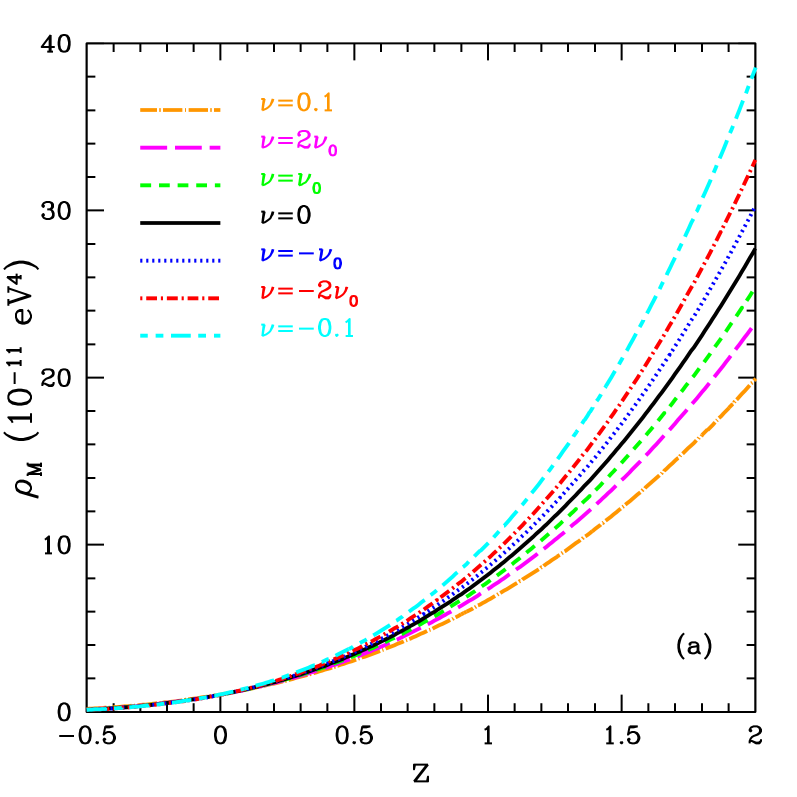
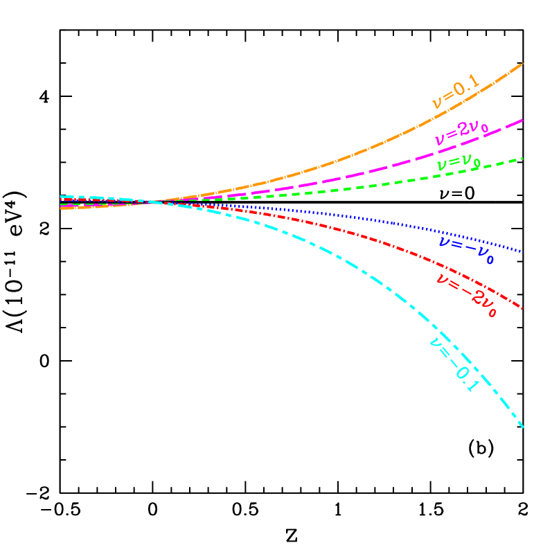
Figure 1: (a),(b) Future and past evolution of the matter density $\rho_{M}(z;\nu)$ and the cosmological constant $\Lambda(z;\nu)$ for a flat universe ($k=0$) and for different values of the fundamental parameter $\nu$ of our model ($\nu_{0}$ is defined in Eq.(45)). In both cases $\Omega_{M}^{0}=0.3$ and $\Omega_{\Lambda}^{0}=0.7$. The solid line represents the standard model case ($\Lambda={\rm const.}$), whereas the various kinds of dots/dashes represent different amounts of evolution of $\Lambda$ [30].

Figure 2: Evolution of the deceleration parameter, $q$, for a flat universe ($k=0$) with $\Omega_{M}^{0}=0.3$ and $\Omega_{\Lambda}^{0}=0.7$. We see that the transition from a decelerated ($q>0$) to an accelerated ($q<0$) universe takes place earlier in time (larger redshifts) for larger $\nu>0$ (see text for the exact values) [30].

In the phenomenologically most interesting case $\,|\nu|<1\,$ we always have a null density of matter and a finite (positive) CC in the long term future, while for the far past yields $\,\Lambda=\pm\infty\,$ depending on the sign of $\,\nu$. In all these situations the matter density safely tends to $\,+\infty$. One may worry whether having infinitely large CC and matter density in the past may pose a problem to structure formation. From Fig. 1a,b it is clear that there should not be a problem at all since in our model the CC remains always smaller than the matter density in the far past, and in the radiation epoch $z>1000$ we reach the safe limit (44). Actually the time where $\Lambda(z;\nu)$ and $\rho_{M}(z;\nu)$ become similar is very recent.

We may consider another relevant exponent describing how the universe evolves, the deceleration parameter q [1]. This one is fully sensitive to the kind of high-z SNe Ia data under consideration. By definition,

$$q(z;\nu)=-\frac{\ddot{a}}{a\,H^{2}(z;\nu)}=\,-1-\frac{\dot{H}}{H^{2}}\,=\,-1+\frac{1}{2}\,(1+z)\,\frac{1}{H^{2}(z;\nu)}\,\frac{dH^{2}(z;\nu)}{dz}\,,$$ (46)

where the $\nu$-dependent Hubble parameter $H^{2}(z;\nu)$ is given in Eq. (34). It is interesting to look at the deviations of the deceleration parameter with respect to the standard model. It is well-known that there are already some data on Type Ia supernovae located very near the critical redshift $z^{*}$ where the universe changed from deceleration to acceleration [42]. But of course the precise location of $z^{*}$ depends on the FLRW model and variations thereof. In our case $\,z^{*}\,$ should depend on our cosmological index $\nu$, i.e. $z^{*}=z^{*}(\nu)$. For simplicity in the presentation, let us consider the flat case. The transition point between accelerated and decelerated expansion is a function of $\,\nu\,$: the more negative is $\,\nu$, the more delayed is the transition (closer to our time)– see Fig. 2. If $\,\nu>0$, the transition occurs earlier (i.e. at larger $z$). While in the standard case, and for a flat universe, the transition takes place at redshift

$$z^{*}=-1+\sqrt[3]{2\,\frac{\Omega_{\Lambda}^{0}}{\Omega_{M}^{0}}}\simeq 0.67\,,$$ (47)

it would have occurred at $z=0.72$ and $z=0.78$ for $\nu=\nu_{0}$ and $\nu=2\nu_{0}$ respectively, and at $z=0.63$ and $z=0.59$ for $\nu=-\nu_{0}$ and $\nu=-2\nu_{0}$ (Cf. Fig. 2). For $\nu=(-0.1,+0.1)$ the effect is quite large, namely the transition would be at $z=(0.53,0.91)$ and hence there is a correction of $(-21\%,+36\%)$ with respect to the standard case.

Distribution	Data	Prior $\sigma_{\Omega_{M}}$	$\nu$	$\sigma_{\nu}$
SNAP	50 SNe $0<z<0.2$
(1 year)	1800 SNe $0.2<z<1.2$
	50 SNe $1.2<z<1.4$
	15 SNe $1.4<z<1.7$	None	$0.1$	$\pm 0.10$
SNAP	as above	0.03	$0.1$	$\pm 0.06$
SNAP	3 years	None	$0.1$	$\pm 0.06$
SNAP	3 years	0.03	$0.1$	$\pm 0.04$
Distr.1	50 SNe $0<z<0.2$
	2000 SNe $0.2<z<1.7$	0.03	$0.1$	$\pm 0.05$
Distr.2	250 SNe $0<z<1$
	1750 SNe $1<z<2$	0.03	$0.1$	$\pm 0.02$

Table 1: Determination of $\nu$ with SNAP data and with other two distributions. In all cases we assume a flat universe. When a prior on $\Omega_{M}$ and its error is added we use $\Omega_{M}=0.3\pm 0.03$  [30].

It should be clear that our approach based on a variable CC departs from all kind of quintessence-like approaches, in which some slow–rolling scalar field $\chi$ substitutes for the CC. In these models, the dark energy is tied to the dynamics of the self-conserved $\chi$ field; i.e. in contrast to (7) there is no transfer between $\chi$-dark energy and ordinary forms of energy. The phenomenological equation of state is defined by $p_{\chi}=w_{\chi}\,\rho_{\chi}$. The term $-2\,\Lambda$ on the r.h.s. of Eq. (6) must be replaced by $\rho_{\chi}+3\,{p}_{\chi}=(1+3\,w_{\chi})\rho_{\chi}$. In order to get accelerated expansion in an epoch characterized by $p=0$ and $\rho\rightarrow 0$ in the future, one must require $-w_{-}\leq w_{\chi}\leq-1/3$, where usually $w_{-}\geq-1$ in order to have a canonical kinetic term for $\chi$ . The particular case $w_{\chi}=-1$ corresponds to a quintessence field exactly mimicking the cosmological constant term. In fact, for a cosmological term $\Lambda$, whether constant or variable, the only possible equation of state is the one corresponding to $w_{\Lambda}=-1$, as it obvious from the definition of $\tilde{T}_{\mu\nu}$ in Eq. (2). Although $p_{\chi}$ and $\rho_{\chi}$ are related to the energy-momentum tensor of $\chi$, the dynamics of this field is unknown because the quintessence models do not have an explanation for the value of the CC. Therefore, the barotropic index $w_{\chi}$ is not known from first principles. In particular, one cannot exclude it may have a redshift dependence, which can be parametrized with two parameters as follows:

$$\frac{p_{\chi}}{\rho_{\chi}}\equiv w_{\chi}=w_{0}+w_{1}(1-a)=w_{0}+w_{1}\frac{z}{1+z}\,.$$ (48)

Finding a non-vanishing value of $w_{1}$ implies a redshift evolution of the equation of state for the $\chi$ field  [5]. For completeness, consider the modification on the Hubble parameter introduced by quintessence models. In this case, and in the flat case, it is easy to see that

$$H^{2}(z;w_{0},w_{1}) = H_{0}^{2}\,\left\{\Omega_{M}^{0}\,(1+z)^{3}\right.$$ (49)

$$+\left.(1-\Omega_{M}^{0})(1+z)^{3(1+w_{0}+w_{1})}\,\exp\left[-3\,w_{1}\,\frac{z}{1+z}\right]\right\}\,.$$

This equation reduces to the standard one (36) for $w_{\chi}=-1$ ($w_{0}=-1,w_{1}=0$), as expected. Comparison between (49) and (35) can be useful to identify the differences between RG models and quintessence models of the dark energy.

Fitting cosmological models to high-z supernovae data is usually performed via the so-called magnitude-redshift relation [2, 3]. One starts from the notion of luminosity distance, $d_{L}$  related to the received flux ${\cal{F}}$ and the absolute (intrinsic) luminosity ${\cal{L}}$ through the geometric definition [1]:

$${\cal{F}}=\frac{{\cal{L}}}{4\pi d_{L}^{2}}\,.$$ (50)

Then the logarithmic relation between flux and the (theoretical) apparent magnitude reads

$$m^{th}(z,H_{0},\Omega_{M}^{0},\Omega_{\Lambda}^{0})\,=\,{\cal{M}}\,+\,5\log_{10}\left[H_{0}\,d_{L}(z,H_{0},\Omega_{M}^{0},\Omega_{\Lambda}^{0})\right]\,,$$ (51)

where $M$ is the absolute magnitude (believed to be constant for all Type Ia supernovae, assuming they are real “standard candles”), and

$${\cal{M}}=M-5\log_{10}H_{0}\,+\,25=M-5\log_{10}h_{0}\,+\,42.38\,.$$ (52)

The model dependence is encoded in the luminosity-distance function $d_{L}=d_{L}(z,H_{0},\Omega_{M}^{0},\Omega_{\Lambda}^{0})$, given in our case by [30]

$$d_{L}(z,H_{0},\Omega_{M}^{0},\Omega_{\Lambda}^{0};\nu)=\frac{1+z}{H_{0}\sqrt{|\Omega_{K}^{0}|}}\ \Psi\left(\sqrt{|\Omega_{K}^{0}|}\int_{0}^{z}{\frac{H_{0}~{}dz^{\prime}}{H(z^{\prime},\Omega_{M}^{0},\Omega_{\Lambda}^{0};\nu)}}\right)\,,$$ (53)

with

$$\Psi(x)=\left\{\begin{array}[]{lr}\sin{x},~{}~{}~{}\Omega_{K}^{0}<0\\ x,~{}~{}~{}~{}~{}~{}~{}~{}\Omega_{K}^{0}=0\\ \sinh{x},~{}~{}\Omega_{K}^{0}>0\,.\end{array}\right.$$ (54)

Here the expansion rate $H(z,\Omega_{M}^{0},\Omega_{\Lambda}^{0};\nu)$ is given by Eq. (34). In the flat case it reduces to the two-parameter function (35), and in quintessence models to the three-parameter function (49). Usually a prior on $\Omega_{M}^{0}$ (from cluster dynamics) can be accepted (e.g. $\Omega_{M}^{0}=0.3$), which narrows down the number of parameters to one (RG) and two (quintessence).

We can use the magnitude-redshift relation defined above to test various distributions, including the one foreseen by SNAP [43]. In order to determine the cosmological parameters we use a $\chi^{2}$-statistic test, where $\chi^{2}$ is defined by the difference between the theoretical apparent magnitude and the observed one (see Ref. [30] for details). The idea is that the difference between models grows with redshift. The existing sample of SN Ia data is amply compatible with $\nu\neq 0$, but it does not pin down a narrow interval of values for this parameter. Trying, however, over several large (simulated) distributions of supernovae, and marginalizing over ${\cal M}$, one obtains the results shown in Table 1. Distribution 1 is very similar to the SNAP one but with most of the data homogeneously distributed between $z=0.2$ and $z=1.7$. Distribution 2 extends data up to redshift $z=2$. We see that we can determine $\nu$ to within $\pm(20-60)\%$ for $\nu=0.1$, depending on the distribution. (Smaller values of $\nu$ imply smaller precision.) The situation is similar to the determination of the evolution of the equation of state, Eq. (48). Indeed, if one performs a general (model-independent) fit of the present SN Ia data to quintessence models, leaving free the two parameters $w_{0}$ and $w_{1}$ in Eq. (48), one finds that the values $w_{0}>-1/3$ (decelerated universe) are ruled out at a high significance level (for $\Omega_{M}^{0}<0.4$), thereby supporting the existence of dark energy. Nevertheless, the very same fit is highly insensitive to $w_{1}$ [39, 16]. On the other hand SNAP will be able to determine $(\Omega_{M}^{0},w_{0})$ to within small errors $(3\%,5\%)$, and will significantly improve the determination of the time-variation parameter $w_{1}$, but only up to $30\%$ at most (each parameter being marginalized over others) [45]. Moreover, the degeneracies among their combinations weaken substantially the tightness of these bounds.

5 Concluding remarks

We have considered a Friedmann-Lemaître-Robertson-Walker model with time-evolving cosmological term: $\Lambda=\Lambda(t)$. The evolution of the CC is due to quantum effects that can be described within the Renormalization Group (RG) approach. The RG scale $\mu$ is identified with the Hubble parameter $H$ at the corresponding epoch, as first proposed in [21]. Although the $\beta_{\Lambda}$-function for $\Lambda$ is just proportional to the fourth power of the masses in the UV regime, the phenomenon of decoupling in QFT leads to an inverse power suppression by the heavy masses at low energies (IR regime). Thus, in the present day universe, one may expect a modified RG equation characterized by a “soft decoupling” behaviour $\beta_{\Lambda}\sim H^{2}M^{2}$ [21, 28, 29, 30]. The effective mass scale $M$ (25) summarizes the presence of the heavy degrees of freedom. This peculiar form of decoupling can be envisaged from:  i) the Appelquist-Carazzone (AC)-decoupling theorem,  ii) general covariance of the effective action, and also from  iii) the non-fine-tuning hypothesis on the $n=1$ terms of $\beta_{\Lambda}$ – Cf. Eq. (21)-(23)– which insures that the coefficient of the quadratic contribution $H^{2}M^{2}$ does not vanish. This particular form of decoupling is a specific feature of the CC because it is of dimension four. There is no other parameter either in the SM or in GUT models with such property.

In constructing this semiclassical “RG-cosmology” we have explored the possibility that the heaviest d.o.f. may be associated to particles having the masses just below the Planck scale, hence $M$ is of order $M_{P}$. This assumption is essential to implement the soft decoupling hypothesis within the $\mu=H$ setting, for the present value of $\,H_{0}^{2}M^{2}\,$ is just of the order of the CC. This fact insures a smooth running of the cosmological term around the present time. In this model the $\beta_{\Lambda}$-function has only one arbitrary parameter $\,\nu\,$ (27) proportional to the dimensionless ratio $M^{2}/M_{P}^{2}$, and as a result the model has an essential predictive power. In general we expect $\,|\nu|\ll 1\,$ from phenomenological considerations, mainly based on the most conservative hypotheses on nucleosynthesis.

As the variation of the CC is attributed, in this model, to the “relic” quantum effects associated to the decoupling of the heaviest degrees of freedom below the Planck scale, a time dependence of the CC may be achieved without resorting to scalar fields mimicking the cosmological term (“quintessence”) or to modifications of the structure of the SM of the strong and electroweak interactions and/or of the gravitational interactions. This proposal, therefore, offers an excellent opportunity to explore the existence of sub-Planck physics in direct cosmological experiments, such as SNAP (and the very high–z SNe Ia data to be obtained with HST). For $\nu\lesssim 0.1$ corrections to some FLRW cosmological parameters become as large as $50\%$ or more, which could not be missed by these experiments.

Whether this RG-cosmology can be easily distinguished from quintessence models requires further considerations along the lines of previous studies on evolving dark energy  [39, 16]. The present model, however, can elude some of the difficulties (related to the degeneracies of the kinematical and geometrical measurements [16]), in that we predict not only an evolving vacuum energy, but also a correlated ($\nu$-dependent) departure of the matter-radiation density from the standard model prediction. From a more fundamental point of view, the sole fact that our FLRW scenario with running cosmological constant can compete on the same footing with quintessence models shows that standard quantum field theory in curved space-time may contain the necessary ingredients from which one can build up a time-evolving cosmological term without need of artificial (“just so”) scalar fields. Both types of models can be thoroughly checked by the SNAP and upgraded HST experiments [43]. If these experiments will detect the redshift dependence of the CC similar to that which is predicted in our work, we may suspect that some relevant physics is going on just below the Planck scale. If, on the contrary, they unravel a static CC, this may imply the existence of a desert in the particle spectrum below the Planck scale, which would be no less noticeable. In this respect let us not forget that the popular notion of a GUT (perhaps in the form of string physics) near the Planck scale remains, at the moment, as a pure (though very much interesting!) theoretical speculation, which unfortunately is not supported by a single piece of experimental evidence up to now. Our framework may allow to explore hints of these theories directly from astrophysical/cosmological experiments which are just round the corner. If the results are positive, it would suggest a direct link between the largest scales in cosmology and the shortest distances in high energy physics.

Acknowledgments. Authors are thankful to E.V. Gorbar, B. Guberina, M. Reuter, H. Stefancic and A. Starobinsky for fruitful discussions. We thank C. España-Bonet and P. Ruiz-Lapuente for their collaboration in the numerical analysis. The work of I.Sh. has been supported by the research grant from FAPEMIG (MG, Brazil) and by the fellowship from CNPq (Brazil). The work of J.S. has been supported in part by MECYT and FEDER under project FPA2001-3598. J.S. is grateful to the organizers of the workshop for the invitation to the conference and for financial support.

References

- [1] P.J.E. Peebles, Principles of Physical Cosmology (Princeton Univ. Press, 1993); T. Padmanabhan, Structure Formation in the Universe (Cambridge Univ. Press, 1993); E.W. Kolb, M.S. Turner, The Early Universe (Addison-Wesley, 1990); J.A. Peacock, Cosmological Physics (Cambridge Univ. Press, 1999); L. Bergstrom, A. Goobar, Cosmology and Particle Astrophysics (John Wiley & Sons, 1999); A. R. Liddle, D.H. Lyth, Cosmological Inflation and Large Scale Structure (Cambridge Univ. Press, 2000).
- [2] S. Perlmutter et al. (the Supernova Cosmology Project), Astrophys. J. 517 (1999) 565.
- [3] A.G. Riess et al. (the High–z SN Team), Astronom. J. 116 (1998) 1009.
- [4] P. de Bernardis et al., Nature 404 (2000) 955; C.B. Netterfield et al. (Boomerang Collab.), Astrophys. J. 571 (2002) 604, astro-ph/0104460; N.W. Halverson et al., Astrophys. J. 568 (2002) 38, astro-ph/0104489.
- [5] C.L. Bennett et al., astro-ph/0302207; D.N. Spergel et al., astro-ph/0302209.
- [6] A.H. Guth, Phys. Rev. 23D (1981) 347; see also the review A.H. Guth, Phys. Rept. 333 (2000) 555.
- [7] A. Blanchard, M. Douspis, M. Rowan-Robinson, S. Sarkar, An alternative to the ‘Concordance Model’, astro-ph/0304237; see also S. Sarkar, these proceedings.
- [8] Ya.B. Zeldovich, Letters to JETPh. 6 (1967) 883.
- [9] ALEPH, DELPHI,L3, OPAL Collab. and the LEP Higgs Working Group, CERN-EP/2001-055, hep-ex/0107030.
- [10] S. Weinberg, Rev. Mod. Phys., 61 (1989); ibid. Relativistic Astrophysics, ed. J.C. Wheeler and H. Martel, Am. Inst. Phys. Conf. Proc. 586 (2001) 893, astro-ph/0005265.
- [11] V. Sahni, A. Starobinsky, Int. J. of Mod. Phys. 9 (2000) 373, astro-ph/9904398; S.M. Carroll, Living Rev. Rel. 4 (2001) 1 astro-ph/0004075; T. Padmanabhan, Phys. Rept. 380 (2003) 235, hep-th/0212290; M.S. Turner, Int. J. Mod. Phys. A17 (2002) 3446, astro-ph/0202007; J. Solà, Nucl. Phys. Proc. Suppl. 95 (2001) 29, hep-ph/0101134.
- [12] A.D. Dolgov, in: The very Early Universe, Ed. G. Gibbons, S.W. Hawking, S.T. Tiklos (Cambridge U., 1982); F. Wilczek, Phys. Rep. 104 (1984) 143.
- [13] R.D. Peccei, J. Solà and C. Wetterich, Phys. Lett. B 195 (1987) 183; L.H. Ford, Phys. Rev. D 35 (1987) 2339; C. Wetterich, Nucl. Phys. B 302 (1988) 668; J. Solà, Phys. Lett. B 228 (1989) 317; J. Solà, Int.J. Mod. Phys. A5 (1990) 4225; A.D. Dolgov, M. Kawasaki, Stability of a cosmological model with dynamical cancellation of vacuum energy, astro-ph/0310822.
- [14] R.R. Caldwell, R. Dave, P.J. Steinhardt, Phys. Rev. Lett. 80 (1998) 1582; P.J.E. Peebles, B. Ratra, Astrophys. J. Lett. 325 L17 (1988).
- [15] P.J.E. Peebles, B. Ratra, Rev. Mod. Phys. 75(2003) 599, astro-ph/0207347.
- [16] T. Padmanabhan, T.R. Choudhury, Mon. Not.Roy. Astron. Soc. 344 (2003)823, astro-ph/0212573; T. D. Saini, T. Padmanabhan, S. Bridle, Mon. Not.Roy. Astron. Soc. 343 (2003) 533, astro-ph/0301536.
- [17] E. Witten, in: Sources and detection of dark matter and dark energy in the Universe, ed. D.B. Cline (Springer, Berlin, 2001), p. 27. hep-ph/0002297; L. Randall and R. Sundrum, Phys. Rev. Lett. 83 (1999) 4690; R. Gregory, V.A. Rubakov and S.M. Sibiryakov, Phys. Rev. Lett. 84 (2000) 5928.
- [18] J. D. Barrow, F. J. Tipler, The Anthropic Cosmological Principle (Clarendon Press, Oxford, 1986); S. Weinberg, Phys. Rev. Lett. 59 (1987) 2607; Phys. Rev. D61 (2000) 103505; J.F. Donoghue, J. High Energy Phys. 0008 (2000) 022.
- [19] R. Sundrum, Fat gravitons, the cosmological constant and sub-millimeter tests, hep-th/0306106.
- [20] J. Yokoyama, Phys. Rev. Lett. 88 (2002) 151302, hep-th/0110137.
- [21] I. Shapiro and J. Solà, J. High Energy Phys. 0202 (2002) 006, hep-th/0012227.
- [22] I. Shapiro and J. Solà, Phys. Lett. B 475 (2000) 236, hep-ph/9910462.
- [23] N.D. Birrell and P.C.W. Davies, Quantum Fields in Curved Space, Cambridge Univ. Press (Cambridge, 1982).
- [24] I.L. Buchbinder, S.D. Odintsov and I.L. Shapiro, Effective Action in Quantum Gravity, IOP Publishing (Bristol, 1992).
- [25] A.M. Polyakov, Int. J. Mod. Phys. 16 (2001) 4511, and references therein; I.L. Shapiro, Phys. Lett. B 329 (1994) 181.
- [26] A. Babic, B. Guberina, R. Horvat and H. Stefancic, Phys. Rev. D65 (2002) 085002; B. Guberina, R. Horvat, H. Stefancic Phys. Rev. D67 (2003) 083001.
- [27] E. Bentivegna, A. Bonanno, M. Reuter, Confronting the IR fixed point cosmology with high redshift supernovae data, astro-ph/0303150; A. Bonanno, M. Reuter, Phys. Rev. D 65 (2002) 043508; ibid astro-ph/0210472, and references therein.
- [28] I.L. Shapiro, J. Solà, C. España-Bonet, P. Ruiz-Lapuente, Variable cosmological constant as a Planck scale effect, Phys. Lett. B 574 (2003) 149, astro-ph/0303306.
- [29] I.L. Shapiro and J. Solà, Cosmological constant, renormalization group and Planck scale physics, hep-ph/0305279, to appear in Nucl. Phys. B Proc. Supp.
- [30] C. España-Bonet, P. Ruiz-Lapuente, I.L. Shapiro, J. Solà, Testing the running of the cosmological constant with Type Ia Supernovae at high z, hep-ph/0311171, to appear in JCAP.
- [31] J. Collins, Renormalization, (Cambridge Univ. Press, 1987); L. Brown, Quantum Field Theory (Cambridge Univ. Press, 1992).
- [32] A. V. Manohar, Effective field theories, in: Schladming 1996, Perturbative and nonperturbative aspects of quantum field theory, hep-ph/9606222.
- [33] T. Appelquist and J. Carazzone, Phys. Rev. D11 (1975) 2856.
- [34] I.L. Shapiro and J. Solà, Phys. Lett. B 530 (2002) 530, hep-ph/0104182; ibid. A modified Starobinsky’s model of inflation: anomaly-induced inflation, SUSY and graceful exit, in: Proc. of SUSY 02 (DESY, Hamburg, 2002) p. 1238, Eds. P. Nath, P.M. Zerwas, hep-ph/0210329; I.L. Shapiro, Int. J. Mod. Phys. D11 (2002)1159, hep-ph/0103128 .
- [35] A.A. Starobinski, Phys. Lett. 91B (1980) 99; JETP Lett. 34 (1981) 460
- [36] E.V. Gorbar, I.L. Shapiro, J. High Energy Phys. 02 (2003) 021, hep-ph/0210388 and J. High Energy Phys. 06 (2003) 004, hep-ph/0303124.
- [37] H. Stefancic, astro-ph/0311247.
- [38] A.M. Pelinson, I.L. Shapiro, F.I. Takakura, Nucl. Phys. 648B (2003) 417, astro-ph/0208184.
- [39] J. A. Frieman, D. Huterer, Eric V. Linder, M. S. Turner, Phys. Rev. D67 (2003) 083505, astro-ph/0208100.
- [40] O. Bertolami, Nuovo Cimento B93 (1986) 36; M. Reuter, C. Wetterich, Phys. Lett. B 188 (1987) 38; J.C. Carvalho, J.A.S. Lima, I. Waga, Phys. Rev. D46 (1992) 2404; L.M. Salim, I. Waga, Class. Quant. Gravit. 10 (1993) 1767; C. Wetterich, Astron. Astrophys. 301 (1995) 321; T. Singh, A. Beesham, Gen. Rel. Grav. 32 (2000) 607, A. Arbab, A. Beesham, Gen. Rel. Grav. 32 (2000) 615; R.G. Vishwakarma, Class. Quant. Grav 18 (2001) 1159; H. Stefancic, astro-ph/0311247.
- [41] J.M. Overduin, F. I. Cooperstock, Phys. Rev. D58 (1998) 043506, and references therein.
- [42] A.G. Riess et al., Astrophys.J. 560 (2001) 49.
- [43] See all the information in: http://snap.lbl.gov/.
- [44] R.R. Caldwell, Phys. Lett. B 545 (2002) 23; H. Stefancic, astro-ph/0310904.
- [45] E. V. Linder AIP Conf. Proc., 655 (2003) 193, astro-ph/0302038.