Stellar collisions during binary–binary and binary–single star interactions

Abstract

Physical collisions between stars occur frequently in dense star clusters, either via close encounters between two single stars, or during strong dynamical interactions involving binary stars. Here we study stellar collisions that occur during binary–single and binary–binary interactions, by performing numerical scattering experiments. Our results include cross sections, branching ratios, and sample distributions of parameters for various outcomes. For interactions of hard binaries containing main-sequence stars, we find that the normalized cross section for at least one collision to occur (between any two of the four stars involved) is essentially unity, and that the probability of collisions involving more than two stars is significant. Hydrodynamic calculations have shown that the effective radius of a collision product can be 2–30 times larger than the normal main-sequence radius for a star of the same total mass. We study the effect of this expansion, and find that it increases the probability of further collisions considerably. We discuss these results in the context of recent observations of blue stragglers in globular clusters with masses exceeding twice the main-sequence turnoff mass. We also present Fewbody, a new, freely available numerical toolkit for simulating small-$N$ gravitational dynamics that is particularly suited to performing scattering experiments.

1 Introduction

Close encounters and direct physical collisions between stars occur frequently in globular clusters. For a star in a dense cluster core, the typical collision time can be comparable to the cluster lifetime, implying that essentially all stars could have been affected by collisions (Hills & Day, 1976). Even in moderately dense clusters, collisions can happen frequently during resonant interactions involving primordial binaries (Hut & Verbunt, 1983; Leonard, 1989; Sigurdsson & Phinney, 1993; Davies & Benz, 1995; Sigurdsson & Phinney, 1995; Bacon et al., 1996). In open clusters with significant binary fractions ($\sim 10$% or more), mergers may occur more often through binary–binary interactions than through single–single collisions and binary–single interactions combined (Leonard & Fahlman, 1991). Collisions involving more than two stars can be quite common during binary–single and binary–binary interactions, since the product of a first collision between two stars expands adiabatically following shock heating, and therefore has a larger cross section for subsequent collisions with the remaining star(s).

Collisions and binary interactions strongly affect the dynamical evolution of globular clusters. The formation of more massive objects through mergers tends to accelerate core collapse, shortening cluster lifetimes. On the other hand, mass loss from evolving collision products can indirectly heat the cluster core, thereby postponing core collapse. The realization during the 1990s that primordial binaries are present in globular clusters in dynamically significant numbers has completely changed our theoretical perspective on these systems (Goodman & Hut, 1989; Sigurdsson & Phinney, 1995; Ivanova et al., 2004). Most importantly, dynamical interactions of hard primordial binaries with single stars and other binaries are thought to be the primary mechanism for supporting globular clusters against core collapse (McMillan et al., 1990, 1991; Gao et al., 1991; Hut et al., 1992; Heggie & Aarseth, 1992; McMillan & Hut, 1994; Rasio et al., 2001; Fregeau et al., 2003; Giersz & Spurzem, 2003). Observational evidence for the existence of primordial binaries in globular clusters is now well established (Hut et al., 1992; Cote et al., 1994; Rubenstein & Bailyn, 1997). Recent Hubble Space Telescope (HST) observations have provided direct constraints on the primordial binary fractions in many clusters. For example, the observation of a broadened main sequence in NGC 6752, based on HST-WFPC2 images, suggests that the binary fraction is probably in the range 15%–40% in the inner core (Rubenstein & Bailyn, 1997). Using a similar method, Bellazzini et al. (2002) find that the binary fraction in the inner region of NGC 288 is probably between 10% and 20%, and less than 10% in the outer region. Observations of eclipsing binaries and BY Draconis stars in 47 Tuc yield an estimate of $\sim 13$% for the core binary fraction (Albrow et al., 2001), although a recent reinterpretation of the observations in combination with new theoretical results suggests that this number might be closer to $\sim 5$% (Ivanova et al., 2004). Using HST-WFPC2, Bolton et al. (1999) derive an upper limit of only $\sim 3$% on the binary fraction in the core of NGC 6397.

In this paper, we focus on interactions involving main-sequence (hereafter MS) stars, and the production of blue stragglers (hereafter BSs). BS stars appear along an extension of the MS blue-ward of the turnoff point in the colour–magnitude diagram (CMD) of a star cluster. All observations suggest that they are massive MS stars formed through mergers of two (or more) lower-mass stars. For example, Gilliland et al. (1998) have demonstrated that the masses estimated from the pulsation frequencies of four oscillating BSs in 47 Tuc are consistent with their positions in the CMD. Indirect measurements of BS masses yield values of up to four times the MS turnoff mass, although the uncertainties are significant (Bond & Perry, 1971; Strom et al., 1971; Milone et al., 1992). More recent spectroscopic measurements yield much more precise masses, with one BS in 47 Tuc about twice the MS turnoff mass (Shara et al., 1997), and two in NGC 6397 more than twice the MS turnoff mass (Sepinsky et al., 2000).

Mergers of MS stars can occur in at least two different ways: via physical collisions, or through the coalescence of two stars in a close binary system (Leonard, 1989; Livio, 1993; Stryker, 1993; Bailyn & Pinsonneault, 1995). Direct evidence for binary progenitors has been found in the form of contact (W UMa type) binaries among BSs in many globular clusters (Rucinski, 2000), including low-density globular clusters such as NGC 288 (Bellazzini et al., 2002), NGC 5466 (Mateo et al., 1990), and M71 (Yan & Mateo, 1994), as well as in many open clusters (e.g., Jahn et al., 1995; Kaluzny & Rucinski, 1993; Milone & Latham, 1994). At the same time, strong indication for a collisional origin comes from detections by HST of large numbers of bright BSs concentrated in the cores of some of the densest clusters, such as M15 (de Marchi & Paresce, 1994; Yanny et al., 1994a; Guhathakurta et al., 1996), M30 (Yanny et al., 1994b; Guhathakurta et al., 1998), NGC 6397 (Burgarella et al., 1994), NGC 6624 (Sosin & King, 1995), and M80 (Ferraro et al., 1999). High-resolution HST images reveal that the central density profiles in many of these clusters steadily increase down to a radius of $\sim 0.1\,$pc, with no signs of flattening. Direct stellar collisions should be extremely frequent in such high density environments.

Evidence for the greater importance of binary interactions over direct collisions of single stars for producing BSs in some globular clusters can be found in a lack of correlation between BS specific frequency and cluster central collision rate (de Angeli & Piotto, 2003; Ferraro et al., 2003). More direct evidence comes from the BS S1082 in the open cluster M67, which is part of a wide hierarchical triple system (Sandquist et al., 2003). The most natural formation mechanism is via a binary–binary interaction. There is further evidence in the radial distributions of BSs in clusters. HST observations, in combination with ground-based studies, have revealed that the radial distributions of BSs in the clusters M3 and 47 Tuc are bimodal – peaked in the core, decreasing at intermediate radii, and rising again at larger radii (Ferraro et al., 2004, 1993, 1997). The most plausible explanation is that the BSs at larger radii were formed through binary interactions in the cluster core and ejected to larger radii (Sigurdsson et al., 1994).

In this paper, we perform numerical scattering experiments to study stellar collisions that occur during binary interactions. One approach for attacking the problem is to perform a full globular cluster simulation, taking into account every relevant physical process, including stellar dynamics, stellar evolution, and hydrodynamics. This approach is enticing in its depth, but would certainly yield results with a complicated dependence on the input parameters and physics that would be difficult to disentangle. A simpler approach is to study in detail the scattering interactions that occur between binaries and single stars or other binaries. This approach isolates the relevant physics and produces results that are easier to interpret. Furthermore, the cross sections tabulated will be useful for future analytical and numerical calculations of cluster evolution and interaction rates. For a discussion of the interplay between globular cluster dynamics and stellar collisions, see, e.g., Hurley et al. (2001). For dense globular cluster cores, merger rates via binary stellar evolution can be significantly enhanced by dynamical interactions (Ivanova et al., 2004).

Our paper is organized as follows. In § 2 we summarize previous theoretical work on stellar collisions in binary interactions. In § 3 we describe our numerical method, and introduce the two numerical codes used. In § 4 we test the validity of our numerical method by comparing with previous results. In § 5 we present a systematic study of the dependence of the collision cross section in binary–single and binary–binary interactions on several physically relevant parameters. In § 6 we consider binaries with parameters characteristic of those found in globular clusters, and study the properties of the resulting binaries and triples containing collision products. Finally, in § 7 we summarize and conclude.

2 Previous Work

There now exists a very large body of numerical work on binary–single and, to a lesser extent, binary–binary interactions (see, e.g., Heggie & Hut, 2003, for an overview and references). Hut & Bahcall (1983) performed one of the most extensive early studies of binary–single star scattering for the equal-mass, point-particle case. Mikkola (1983a) performed the first systematic studies of binary–binary interactions in the point-particle limit, first for the case of equal energy binaries, and later for unequal energies (Mikkola, 1984a). He also studied the energy generated in binary–binary interactions in the context of the evolution of globular clusters (Mikkola, 1983b, 1984b). Most numerical scattering experiments have been performed in the point-mass limit, neglecting altogether the effects of the finite size of stars. However, as we summarize below, there are a number of studies that apply approximate prescriptions for dissipative effects and collisions post facto to numerical integrations performed in the point-mass limit but in which pairwise closest approach distances were recorded. There is also one study in which collisions are treated in situ in a simplified manner, and several that perform full smoothed particle hydrodynamics (SPH) simulations of multiple-star interactions (see below).

Hoffer (1983) was the first to study distances of closest approach between stars in both binary–single and binary–binary interactions. He found that roughly 40% of binary–binary encounters in a typical globular cluster core will lead to a physical collision between two stars. Krolik et al. (1984) considered the evolution of a compact binary in a globular cluster core subject to perturbations by single field stars, and found that an induced merger or collision between two stars in a binary–single interaction is likely. Hut & Inagaki (1985) applied a single-parameter, “fully inelastic sphere” collision model after the fact to a large number of binary–single interactions for which distances of closest approach were recorded, and calculated merger rates. McMillan (1986) applied simple prescriptions for the dissipative effects of gravitational radiation, tidal interactions, and physical contact between stars after the fact to a large number of binary–single interactions involving tight binaries. He found that dissipative effects reduce binary heating efficiency in cluster cores by roughly an order of magnitude over that obtained in the point-mass limit. He also found that the most likely outcome of a binary–single interaction involving a tight binary is the coalescence of at least two of the stars. This work was carried further by Portegies Zwart et al. (1997a, b), who included the effects of binary stellar evolution on binary–single interactions. They found that about 20 per cent of encounters between a primordial binary and a cluster star result in collisions, while almost 60 per cent of encounters with tidal-capture binaries lead to collisions. Leonard (1989) performed a small number of binary–binary interactions and recorded close approach distances and calculated ejection speeds of collision products. Leonard & Fahlman (1991) performed the first set of binary–single and binary–binary interactions in which stars were allowed to merge during the numerical integration. They studied the rate of production of BSs in clusters, and performed the first, simplified “population synthesis” study of BSs in clusters. Hills (1991, 1992) considered stars with a range of masses exchanging into binaries, and found the distance of closest approach to be roughly a constant fraction of binary semimajor axis independent of intruder mass, over a wide range of mass ratios. Cleary & Monaghan (1990) performed full SPH simulations of binary–single interactions and showed directly the importance of taking into account the non-zero size of stars. Goodman & Hernquist (1991) and Davies et al. (1993, 1994) performed sets of binary–single and binary–binary interactions with tight binaries in the point-mass limit, and selected a handful to run with a full SPH code. They found that multiple mergers are common. Bacon et al. (1996) performed a large number of binary–binary interactions and presented a survey of close approach cross sections for several sets of physically relevant binary parameters. They also calculated outcome frequencies, studied the properties of the interaction products, and used their results in analytical calculations of interaction rates in globular cluster cores. More recently, Giersz & Spurzem (2003) have incorporated into their Monte-Carlo globular cluster evolution code Aarseth’s NBODY for performing direct integrations of binary interactions. By storing the results of binary interactions that occur during cluster evolution, they have calculated close approach cross sections, and a few differential cross sections.

3 Numerical Method

The scattering experiments presented in this paper were performed primarily using Fewbody, a new numerical toolkit designed for simulating small-$N$ gravitational dynamics, which we describe below. In some cases we also use the scattering facilities of the Starlab software environment (Portegies Zwart et al., 2001). Starlab was used mainly to compare with Fewbody, but in cases where Starlab data were compiled before Fewbody was written, Starlab results were used. In particular, all calculations in § 6 were performed with Starlab.

3.1 Setup

We label the two objects in a scattering experiment 0 and 1. In the case of binary–single scattering, 0 is the binary and 1 is the single star. In the case of binary–binary scattering, 0 and 1 are each binaries. We use the same system of labelling for each binary, so the members of binary $i$ are labelled $i0$ and $i1$. There are several parameters required to uniquely specify a binary–single or binary–binary scattering experiment. To describe the initial hyperbolic (or parabolic) orbit between objects 0 and 1, one needs to specify the relative velocity at infinity $v_{\infty}$, impact parameter $b$, and masses $m_{0}$ and $m_{1}$. To describe the internal properties of each object, one needs to specify the semimajor axes $a_{i}$, eccentricities $e_{i}$, individual masses $m_{ij}$, and stellar radii $R_{ij}$. There are also several phase and orientation angles required for each binary: the orientation of the binary angular momentum vector relative to the angular momentum vector describing the orbit between 0 and 1, given by the polar angle $\theta$ and the azimuthal angle $\phi$; the angle $\omega$ between the binary Runge-Lenz vector and some fiducial vector perpendicular to the binary angular momentum vector (e.g., the cross product of the binary angular momentum and the 0-1 angular momentum); and $\eta$, the mean anomaly of the binary. For all the scattering experiments presented in this paper, these phase and orientation angles are chosen randomly, so that the cross sections calculated represent averages over these quantities. In detail, these angles are given by $\theta=\cos^{-1}(2X-1)$, $\phi=2\pi X$, $\omega=2\pi X$, and $\eta=2\pi X$, where $X$ is a uniform deviate in the range $[0,1)$. In addition, unless otherwise noted, the eccentricity of each binary is chosen from a thermal distribution (Jeans, 1919) truncated at large $e$ such that there is no contact binary. In each scattering experiment, numerical integration is started at the point at which the tidal perturbation ($F_{\rm tid}/F_{\rm rel}$) on a binary in the system reaches $\delta$ (see § 3.3.4).

It is customary to specify the relative velocity at infinity in terms of the critical velocity, $v_{c}$, defined such that the total energy of the binary–single or binary–binary system is zero. For $v_{\infty}>v_{c}$ the total energy of the system is positive, and full ionization is possible. That is, a possible outcome of the scattering experiment is that each star leaves the system unbound from any other with positive velocity at infinity. For $v_{\infty}<v_{c}$, the total energy of system is negative, and the encounters are likely to be resonant, with all stars involved remaining in a small volume for many dynamical time-scales. Defining the total mass $M=m_{0}+m_{1}$ and reduced mass $\mu=m_{0}m_{1}/M$, the critical velocity is

$$v_{c}=\left[\frac{G}{\mu}\left(\frac{m_{00}m_{01}}{a_{0}}\right)\right]^{1/2}$$ (1)

for the binary–single case, and

$$v_{c}=\left[\frac{G}{\mu}\left(\frac{m_{00}m_{01}}{a_{0}}+\frac{m_{10}m_{11}}{a_{1}}\right)\right]^{1/2}$$ (2)

for the binary–binary case. The cross section for outcome X is obtained by performing many scattering experiments out to a maximum impact parameter $b_{\rm max}$ and calculating

$$\sigma_{X}=\pi b_{\rm max}^{2}\frac{N_{X}}{N}\,,$$ (3)

where $N_{X}$ is the number of experiments that have outcome X, and $N$ is the total number of scattering experiments performed. In all cases the maximum impact parameter was chosen large enough to ensure that the full region of interest was sampled. In other words, for $b>b_{\rm max}$, all interactions are fly-by’s in which each binary is only weakly tidally perturbed during the interaction. For calculations performed with Fewbody, $b_{\rm max}$ was chosen to correspond to a pericentre distance of $r_{p}=5(a_{0}+a_{1})$ in the binary–binary case, and $r_{p}=5a$ in the binary–single case. For this value of pericentre distance, the binary eccentricity induced in the fly-by is quite small ($\delta e\ll 1$ for initially circular binaries, and $\delta e/e\ll 1$ for non-circular binaries; see Rasio & Heggie, 1995; Heggie & Rasio, 1996). For calculations performed with Starlab, $b_{\rm max}$ was chosen automatically by using successively larger impact parameter annuli until no relevant outcomes were found (McMillan & Hut, 1996). The uncertainty in the cross section is calculated assuming Poisson counting statistics, so that

$$\Delta\sigma_{X}=\pi b_{\rm max}^{2}\frac{\sqrt{N_{X}}}{N}\,.$$ (4)

In principle, it is necessary to include scattering experiments that result in unresolved outcomes in this uncertainty (see, e.g., Hut & Bahcall, 1983). However, in practice we find that the number of unresolved outcomes is small, and does not significantly contribute to $\Delta\sigma_{X}$.

3.2 Possible Outcomes

The possible outcomes of binary–single and binary–binary scattering interactions are listed in Tables 1 and 2, ordered by the number of collisions, $n_{\rm coll}$. Stars are represented as filled circles, brackets enclose two objects that are bound to each other in a binary, and colons represent physical collision products. In Table 2 we also list the abbreviations used in the paper to refer to certain outcomes. When there are no collisions (as is the case in the point-mass limit), the number of possible outcomes is small, as shown in the $n_{\rm coll}=0$ rows in each table. However, when one considers stars with non-zero radius and allows for the possibility of collisions and subsequent mergers, the total number of outcomes becomes large. Assuming indistinguishable stars, there are six possible outcomes for the binary–single case, and 16 for the binary–binary case. These numbers are evidently increased for distinguishable stars. The software used in this paper distinguishes among all possible outcomes.

3.3 Fewbody

Fewbody is a new numerical toolkit for simulating small-$N$ gravitational dynamics. It is a general $N$-body dynamics code, although it was written for the purpose of performing scattering experiments, and therefore has several features that make it well-suited for this purpose. It can be described succinctly in terms of its key elements.

3.3.1 Adaptive Integration and Regularization

At its core, Fewbody uses the 8th-order Runge-Kutta Prince-Dormand integration method with 9th-order error estimate and adaptive timestep to advance the $N$-body system forward in time. It integrates the usual formulation of the $N$-body equations in configuration space, but allows for the option of global pairwise Kustaanheimo-Stiefel (K-S) regularization (Heggie, 1974; Mikkola, 1985). Global regularization is a coordinate transformation that removes all singularities from the $N$-body equations, making the integration of close approaches, and even collision orbits, much more accurate. It is well-suited for small-$N$ dynamics, since it requires the integration of $\sim N^{2}$ separations instead of $N$ positions, and becomes prohibitively computationally expensive for $N\ga 10$. Although it should in principle make numerical integration more accurate, it was found that the adaptive timestep algorithm alone performed as well as global regularization, in terms of the computational time required for a specified level of energy and angular momentum accuracy. The use of regularization requires extra effort to detect physical collisions, since, with regularization, pericentre is not necessarily resolved by the integrator. For the sake of simplicity, we have chosen not to implement the appropriate technique for detecting collisions with regularization (see § 9.8 of Aarseth, 2003). Furthermore, physical collisions naturally soften the singularities in the non-regularized $N$-body equations by making them physically inaccessible. Regularization was therefore only used to test calculations made in the point-mass limit. For all other calculations the non-regularized integration routine was used.

3.3.2 Classification

Fewbody uses a binary tree algorithm to handle several aspects related to performing scattering experiments. Most importantly, it uses a binary tree algorithm to classify the $N$-body system into a set of independently bound hierarchies. For example, if the outcome of a scattering experiment between two hierarchical triples is a hierarchical triple composed of binaries, Fewbody will classify it accordingly. Fewbody creates the set of binary trees iteratively, according to the following simple rules. First, as shown in Figure 1, any existing set of trees is flattened so that each star in the $N$-body system represents the top-level node of a one-node tree. Next, as shown in Figure 2, the two top-level nodes that are bound to each other with the smallest semimajor axis are replaced by a parent node containing all dynamical information about the centre of mass, as well as all information about the binary’s orbit, including phase. The previous step is repeated, as shown in Figure 3, until no top-level nodes are found to be bound to each other. This algorithm is clearly general in $N$. The resulting set of binary trees is a unique classification of the configuration of the $N$-body system. As described below, the classification is used for determining when an interaction is complete. The binary tree algorithm is also used (with a slightly different set of rules for creating the trees) to make the numerical integration more efficient, as also described below.

3.3.3 Stability

Fewbody assesses the dynamical stability of gravitationally bound hierarchies in an approximate way using the classification just described, and a simple analytical test. There currently exists only one reasonably accurate criterion for the dynamical stability of an $N>2$ gravitational system, the approximate analytical criterion of Mardling & Aarseth (2001) for the dynamical stability of hierarchical triples. Fewbody assesses the stability of each binary tree by applying this criterion at each level in the tree. For example, for a hierarchical quadruple system (which consists of a star in orbit around a hierarchical triple – shown as “[[[$\bullet$ $\bullet$] $\bullet$] $\bullet$]” in Table 2), it first applies the triple stability criterion to the inner triple, then applies it to the “outer” triple, treating the innermost binary as a single object. For the case of a hierarchical quadruple composed of two binaries (“[[$\bullet$ $\bullet$] [$\bullet$ $\bullet$]]” in Table 2), Fewbody uses the additional correction factor presented in § 4.2 of Mardling & Aarseth (2001). The stability of a hierarchical system as determined by this method is only approximate, but, in our experience, seems to work reasonably well. For the particular case of binary–binary scattering, hierarchical triples which appear to be stable are classified as unstable less than roughly one percent of the time.

It should be noted that the stability assessed here is dynamical rather than secular, so, e.g., any resonances that would destroy an otherwise stable hierarchical system are ignored. Such resonances are likely to be important in the more general context of the dynamics of globular clusters and their constituent populations (e.g., Miller & Hamilton, 2002; Ford et al., 2000), but are beyond the scope of the present paper. It should also be noted that our use of binary trees prevents us from recognizing stable three-body systems which are not hierarchical, such as the stable “figure eight” orbit for three stars of comparable mass (Chenciner & Montgomery, 2000; Montgomery, 2001). However, the fraction of strong binary–binary scattering encounters resulting in this configuration is likely to be exceedingly small (Heggie, 2000).

3.3.4 Hierarchy Isolation

Fewbody also uses a binary tree algorithm to speed up numerical integration by isolating from the integrator certain tight binaries and hierarchies that are only very weakly perturbed, yet dominate the calculation by driving down the integration time-scale. It does this by integrating only the top-level nodes (centres of mass) of a set of binary trees created using the algorithm described in § 3.3.2, but subject to a slightly different rule-set. Two top-level nodes can only be replaced by their parent node if: (1) the binary tree represented by the parent node is stable, (2) the tidal perturbation on the outer binary of the tree (the two nodes below the top-level) at apocentre due to all other top-level nodes in the system is less than a specified fraction, $\delta$, of the minimum force between them ($F_{\rm tid}/F_{\rm rel}<\delta$ at apocentre), and (3) the evolution of the binary tree can be treated analytically. The relative force at apocentre is calculated simply as

$$F_{\rm rel}=\frac{Gm_{0}m_{1}}{[a(1+e)]^{2}}\,,$$ (5)

where $m_{0}$ and $m_{1}$ are the masses of the members of the outer binary, $a$ is the semimajor axis, and $e$ is the eccentricity. The tidal force at apocentre is calculated simply as

$$F_{\rm tid}=\sum_{i}\frac{2G(m_{0}+m_{1})m_{i}}{r_{i}^{3}}a(1+e)\,,$$ (6)

where the sum is taken over all other top-level nodes in the system, $m_{i}$ is the mass of the other top-level node, and $r_{i}$ is the distance to the other top-level node. Note that this sum represents the upper limit of the tidal force since it does not take into account relative inclination between the binary and the other top-level nodes.

A binary (or hierarchy) that is isolated from the integrator in this way is treated numerically again when its relative tidal perturbation exceeds $\delta$. This is done by resuming the integration from the previous step (when the hierarchy’s tidal perturbation was less than $\delta$) with the parent node replaced by its child nodes, and orbital phase advanced to the current time. In practice, this algorithm isolates from the integrator mainly weakly-perturbed binaries, and a few extremely hierarchical triples in which the tidal perturbation on the inner binary due to the outer member is very small. For binary–single scattering, hierarchy isolation can speed up the integrations by up to an order of magnitude on average. For binary–binary scattering, especially when the two binaries have very disparate semimajor axes, and hence orbital time-scales, this algorithm can speed up the integrations by a few orders of magnitude on average. The quantity $\delta$ plays the role of an integration tolerance parameter. Larger values of $\delta$ allow hierarchies to be treated analytically more frequently, yielding faster calculations but sacrificing energy accuracy. Smaller values of $\delta$ yield better energy conservation at the expense of computational speed.

3.3.5 Calculation Termination

Fewbody uses the classification and stability assessment techniques outlined above, in combination with a few simple rules to automatically terminate the integration of scattering encounters when they are complete – in other words, when the separately bound hierarchies comprising the system will no longer interact with each other or evolve internally. Integration is terminated when: (1) each pair of top-level nodes has positive relative velocity, (2) the tidal perturbation ($F_{\rm tid}/F_{\rm rel}$) on the outer binary (the two nodes below the top-level) of each tree due to the other top-level nodes is smaller than $\delta$, (3) each tree is dynamically stable (as defined in § 3.3.3), and (4) the $N$-body system composed of the top-level nodes has positive energy. The last condition is required because it is possible for the members of an $N$-body system to be separately unbound and receding from each other, yet for the system as a whole to be bound. Here $\delta$ again plays the role of an accuracy parameter, with smaller $\delta$ yielding more accurate outcome classifications. Since the $N$-body problem is chaotic, with initially neighbouring trajectories in phase space diverging exponentially, the value of $\delta$ should play only a minor role in the statistical accuracy of classifications of outcomes.

3.3.6 Physical Collisions

Fewbody performs collisions between stars in the “sticky star” approximation. In this approximation, stars are treated as rigid spheres with radii equal to their stellar radii. When two stars touch, they are merged with no mass lost, and with linear momentum conserved. (Tidal effects, which may significantly increase the collision rate for close encounters (see, e.g., McMillan, 1986), are beyond the scope of this method, but may be approximated by larger initial effective stellar radii.) The radius of the merger product is set to

$$R_{\rm merger}=f_{\rm exp}(R_{1}+R_{2})\,,$$ (7)

where $R_{1}$ and $R_{2}$ are the radii of the merging stars, and $f_{\rm exp}$ is an expansion factor. To determine a reasonable value for $f_{\rm exp}$, one must consider the relevant time-scales involved. The characteristic time-scale of a typical binary scattering encounter in a globular cluster core is between $\sim 10\,\mbox{yr}$ for a fly-by and $\la 10^{4}\,\mbox{yr}$ for a resonant encounter, while the thermal time-scale of a $\sim 1\,M_{\sun}$ MS star is $\sim 10^{7}\,\mbox{yr}$. Therefore, it is invalid to treat merger products as rejuvenated (“reborn”) MS stars ($f_{\rm exp}=1$) during scattering encounters. The hydrodynamical time-scale is $\sim 1\,\mbox{hr}$, so it is more accurate to treat merger products as hydrodynamically settled. SPH simulations show that $f_{\rm exp}$ should be in the range 2–30, depending on the relative orientations of the two stars before collision (Lombardi et al., 2003). These simulations also show that the amount of mass lost in the types of collisions characteristic of globular clusters is typically of order 1%, so our assumption of zero mass loss is a reasonable first approximation.

Collision products are likely to have significant rotation and be non-spherical. Furthermore, it is not clear that the value of the expansion parameter for the merger of two pristine MS stars should be the same as that for mergers involving collision products. Thus $f_{\rm exp}$ should be considered an effective quantity, averaged over many collisions. A more realistic approach that adopts several separate parameters is in principle possible, but beyond the scope of the current paper.

3.3.7 General Availability

Fewbody is freely available for download on the web, licensed under the GNU General Public License (GPL). It contains a collection of command line utilities that can be used to perform individual scattering and $N$-body interactions, but is more generally a library of functions that can be used from within other codes. Its facilities make it aptly suited for performing scattering interactions from within larger numerical codes that, e.g., calculate cross sections, or evolve globular clusters via Monte-Carlo techniques.

Available along with Fewbody, there is an OpenGL-based visualization tool called GLStarView that can be used to view $N$-body interactions as they are being calculated by Fewbody, in an immersive, 3-D environment. GLStarView has proven to be a valuable aid in developing our understanding and physical intuition of binary interactions.

3.4 Starlab

Starlab is a collection of modular software tools designed to simulate the evolution of dense stellar systems and analyse the resulting data (see Portegies Zwart et al., 2001, for a detailed description). It is freely available on the web. It consists of a library of programs for performing stellar dynamics, stellar evolution, and hydrodynamics, together with a set of programs acting as bridges between them. They may be combined to study all aspects of the evolution of $N$-body systems. For this paper, we use the three-body scattering facility scatter3 and the general $N$-body scattering facility scatter from version 3.5 of Starlab, along with sigma3 and sigma for the automated calculation of cross sections.

4 Tests and Comparisons

To assess the validity of calculations performed with Fewbody, we have compared the results of several scattering experiments with the results of previous studies. For general binary–single interactions, we have compared our results with those of Hut & Bahcall (1983); for general binary–binary, Mikkola (1983a); and for detecting close approach distances, we have compared with binary–binary calculations performed by Bacon et al. (1996). The scattering facilities in Starlab have been used extensively and tested thoroughly (see, in particular, Gualandris et al., 2004). However, there has only been one reported comparison between the three-body scattering routine and the $N$-body routine in the literature (Gualandris et al., 2004). Below, we perform a new test and show that the two routines agree at a basic level.

4.1 General binary–single comparison

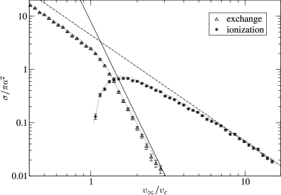
Figure 4: Comparison of Fewbody with Figure 5 of Hut & Bahcall (1983): total cross sections for binary–single scattering for the equal-mass, zero eccentricity, point-particle case. A total of $8\times 10^{5}$ scattering experiments were used to create this figure. The dotted lines represent the data from Hut & Bahcall (1983), while the straight solid and dashed lines are the theoretically predicted cross sections for ionization and exchange from the same paper. Data points are from Fewbody. The agreement between the two is excellent.

Hut & Bahcall (1983) performed one of the most extensive early studies of binary–single star scattering for the equal-mass, point-particle case. Figure 4 shows a comparison of the results of $8\times 10^{5}$ scattering interactions calculated using Fewbody with their Figure 5. Plotted are the total dimensionless cross sections ($\sigma/(\pi a^{2})$, where $a$ is the binary semimajor axis) for ionization (shown by star symbols) and exchange (triangles) as a function of $v_{\infty}/v_{c}$, for the equal-mass, zero eccentricity, point-particle case. The dotted lines represent the data from their figure (without error bars), while the straight solid and dashed lines are the theoretically predicted cross sections for ionization and exchange from the same paper. The agreement between the two is excellent, although it appears that Hut & Bahcall systematically find a slightly larger cross section for ionization. We note, however, that the two agree at roughly the one-sigma level.

4.2 General binary–binary comparison

The first systematic study of binary–binary scattering was presented by Mikkola (1983a). He considered binaries with equal semimajor axes, and stars of equal mass, in the point-particle limit. We have chosen to compare with Table 5 of Mikkola (1983a), which presents sets of scattering experiments performed for several different values of $v_{\infty}/v_{c}$, with impact parameter chosen uniformly in area out to the maximum impact parameter found to result in a strong interaction (listed in his Table 3). Only strong interactions were counted, and the eccentricities of the binaries were chosen from a thermal distribution. It should be noted, for the sake of completeness, that Mikkola characterised his encounters by their dimensionless energy at infinity, $T_{\infty}$. The relation between $v_{\infty}$ and $T_{\infty}$ is $v_{\infty}/v_{c}=\sqrt{T_{\infty}}$. Mikkola’s classification scheme is similar to Fewbody’s, the two primary differences being: (1) the value of the tidal tolerance, $\delta$, used by Mikkola is $3\times 10^{-4}$, while the Fewbody runs use $\delta=10^{-5}$; and (2) the criterion used to assess the dynamical stability of triples is that of Harrington (1974), a much less accurate stability criterion than the Mardling & Aarseth (2001) criterion used by Fewbody. It is therefore expected that the classification of Fewbody is more accurate. The binary–binary scattering encounters are classified into five different outcomes. The label “undecided” represents an encounter that was deemed to be unfinished after a preset amount of computation time – in other words, it could not be classified into one of the four categories of “exchange”, “triple”, “single ionization”, or “full ionization”. These four outcomes are described in the $n_{\rm coll}=0$ rows of Table 2. Table 3 compares results from Fewbody with Mikkola’s Table 5. The comparison is also shown graphically in Figure 5.

Several comments are in order. Looking at the “undecided” column in Table 3, it is clear that Fewbody resolves more encounters than Mikkola, yielding roughly half as many undecided encounters. This is a result of both the increased power of modern computers – resonant encounters can be integrated longer, and one can use smaller $\delta$ – and the more accurate triple stability criterion available today. In the next column, labelled “exchange”, it is clear that Mikkola finds many more exchange encounters than Fewbody. This is thought to be primarily because in this column Mikkola’s data include strong interactions, which result not only in exchange, but also in preservation. We have not included this type of outcome in the Fewbody results because it would have been cumbersome to implement Mikkola’s test for a strong interaction. The next column, labelled “triples”, shows that Mikkola regularly classifies more triples as stable than Fewbody. This results in fewer outcomes labelled as “single ionization”, since the test for single ionization occurs after that of triple stability in Mikkola’s code. Full ionizations can only occur when the total energy of the system is greater than or equal to zero ($v_{\infty}/v_{c}\geq 1$). There is a large discrepancy in the number of full ionizations for $v_{\infty}/v_{c}=1.225$. We are not quite sure of the underlying reason for the discrepancy, but think it may be due to the tidal tolerance used, which differs by more than an order of magnitude between the two methods. Aside from the systematic discrepancies pointed out above, the two methods agree at a reasonable level, given the differences between them. This is especially clear from Figure 5. For all outcomes except full ionization, the methods agree at roughly the two-sigma level (the uncertainties shown are one-sigma).

4.3 Comparison for close-approach distances

Bacon et al. (1996) presented a more recent and detailed study of binary–binary interactions in the point-particle limit, in which close-approach distances were recorded and used to calculate cross sections. In the scattering experiment we have chosen for comparison, each binary had equal semimajor axis ($a_{0}=a_{1}=a$) and zero eccentricity, and all stars had equal mass. The impact parameter was chosen uniformly in area out to the maximum impact parameter given by $b_{\rm max}/a=C/v_{\infty}+D$, where $C=5$, and $D=0.6$. This expression for the impact parameter is an extension of that used by Hut & Bahcall (1983), designed to sample strong interactions adequately. For each encounter, the minimum pairwise close approach distance, $r_{\rm min}$, was recorded; and from the set, the cumulative cross section calculated.

Figure 6 shows a comparison with their Figure 4. The circles with error bars represent Fewbody data, while the solid-line broken power-law is the best fit to the results obtained by Bacon et al. (1996). There is clearly a multiple-sigma discrepancy for $r_{\rm min}/a\la 0.01$. The discrepancy results from the lack of use by Bacon et al. (1996) of the appropriate algorithm for detecting close approach distances with regularization (§ 18.4 of Aarseth, 2003). Sigurdsson has resurrected the original code, and performed a recalculation with smaller timesteps. The new result is shown by the dot-dash line. The resulting cross section is closer to the Fewbody result, yet still systematically smaller.

For comparison, we have performed the same calculation using Starlab, shown by the dashed line. The agreement between Fewbody and Starlab is excellent. The only discrepancy between the two occurs at $r_{\rm min}/a\sim 1$, which represents the weak perturbation of binaries due to distant fly-by’s. This discrepancy is most likely due to the differing values of the tidal tolerance used. For the Fewbody runs, the tidal tolerance was $\delta=10^{-5}$, while for the Starlab runs it was $\delta=10^{-6}$, causing Starlab to numerically integrate some weakly-perturbed binaries that Fewbody treated analytically. The result is a slightly larger Starlab cross section for $r_{\rm min}/a\sim 1$, as can be seen in the figure.

We should note that the original calculation of Bacon et al. (1996) was averaged over the range $0.125\leq v_{\infty}/v_{c}\leq 0.25$, while all other results shown in Figure 6 were calculated with $v_{\infty}/v_{c}=0.25$. This cannot account for the discrepancy with the original calculation, since the inclusion of smaller velocities at infinity will result in more resonant interactions, and hence smaller distances of close approach. We have performed calculations with $v_{\infty}/v_{c}=0.125$ and found that the cross section differs from that with $v_{\infty}/v_{c}=0.25$ by no more than a few per cent.

Finally, we remark that the error in the original calculation of Bacon et al. (1996) is only present for small $r_{\rm min}$; many of the conclusions in their paper are not affected by this error.

4.4 Comparison between Starlab’s three-body and $N$-body scattering routines

The scattering facilities in Starlab have been used extensively and tested thoroughly (McMillan & Hut, 1996; Gualandris et al., 2004). However, there is only one reported comparison between scatter3, the three-body scattering routine, and scatter, the $N$-body scattering routine, in the literature (Gualandris et al., 2004). A simple test, tuned to suit the purposes of this paper, is to compare the binaries containing merger products that result from binary–single interactions with those from binary–binary interactions designed to mimic binary–single interactions. An obvious choice for the limiting-case binary–binary interaction is that in which one binary has an extremely small mass ratio. We performed binary–single runs in which each star had mass $M_{\sun}$, radius $R_{\sun}$, the binary had semimajor axis $1\,\mbox{AU}$ and $e=0$, and $v_{\infty}=10\,\mbox{km/s}$. In the binary–binary runs, the binary mimicking the single star had a secondary of mass $10^{-5}\,M_{\sun}$, semimajor axis of $20\,\mbox{AU}$, and $e=0$. The results of $10^{4}$ runs are shown in Figure 7, in which we plot the cumulative fraction of binaries as a function of $r_{p}/a$, where $r_{p}$ is the pericentre distance of the merger binary, and $a$ is the initial binary semimajor axis. The agreement between scatter3 (solid line) and scatter (dashed line) is good, with both yielding merger binaries with $r_{p}$ strongly concentrated between $0.15\,\mbox{AU}$ and $0.3\,\mbox{AU}$.

5 Systematic Study of the Collision Cross Section

To better understand the behavior of the collision cross section, we have systematically studied its dependence on several physically relevant parameters. The understanding gained will allow us to reduce the dimensionality of parameter space that must be sampled when we later consider MS-star binaries with physically motivated parameters.

5.1 Dependence on velocity at infinity

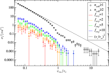
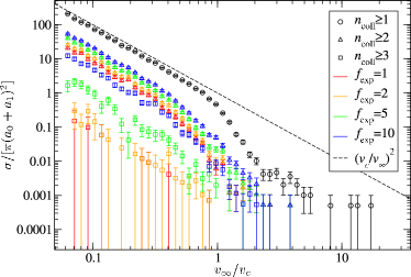
Figure 8: Cross section for physical collisions in binary–single (left) and binary–binary (right) scattering as a function of the relative velocity at infinity, for different values of the expansion parameter, $f_{\rm exp}$. Circles represent outcomes with one or more collisions; triangles, two or more; and squares, three or more. Red represents runs with $f_{\rm exp}=1$; orange, $f_{\rm exp}=2$; green, $f_{\rm exp}=5$; and blue, $f_{\rm exp}=10$. In both experiments (binary–single and binary–binary), each star had mass $M_{\sun}$ and radius $R_{\sun}$, and each binary had semimajor axis $a=1\,\mbox{AU}$ and eccentricity $e=0$. The cross section decreases sharply at the critical velocity, $v_{c}$, above which resonant scattering is forbidden.

The dimensionless collision cross section ($\sigma/(\pi a^{2})$ for binary–single, $\sigma/(\pi(a_{0}+a_{1})^{2})$ for binary–binary) as a function of the relative velocity at infinity, $v_{\infty}/v_{c}$, is shown in Figure 8, for both binary–single interactions (left) and binary–binary interactions (right), for several different values of the expansion parameter, $f_{\rm exp}$. Circles represent outcomes with one or more collisions (two or more stars collide); triangles, two or more (three or more stars collide); and squares, three (four stars collide). Red represents runs with $f_{\rm exp}=1$; orange, $f_{\rm exp}=2$; green, $f_{\rm exp}=5$; and blue, $f_{\rm exp}=10$. In both experiments (binary–single and binary–binary), each star had mass $M_{\sun}$ and radius $R_{\sun}$, and each binary had semimajor axis $a=1\,\mbox{AU}$ and eccentricity $e=0$. The cross section decreases sharply at $v_{\infty}/v_{c}=1$, above which resonant scattering is forbidden, and appears to approach a constant value, consistent with being purely geometrical. In the resonant scattering regime, below $v_{\infty}/v_{c}=1$, the collision cross section follows the form $1/v_{\infty}^{2}$, implying that gravitational focusing is dominant. The $n_{\rm coll}\geq 1$ cross section in the resonant scattering regime is quite high, with $\sigma(v_{\infty}/v_{c})^{2}/(\pi a^{2})\approx 1$ for binary–single and $\sigma(v_{\infty}/v_{c})^{2}/(\pi(a_{0}+a_{1})^{2})\approx 0.8$ for binary–binary.

The $n_{\rm coll}\geq 2$ cross section in the binary–single case is about two to three orders of magnitude below that for $n_{\rm coll}\geq 1$, depending on $f_{\rm exp}$. However, in the binary–binary case, the $n_{\rm coll}\geq 2$ cross section is only down by a factor of a few to 10. The reason for the difference is that in the binary–single case, after one collision occurs, there are only two stars left. The two remaining stars will either be bound in a binary, or unbound to each other in a hyperbolic orbit. In the case of a bound orbit, the two stars are guaranteed to make at least one pericentre passage, and if the merger product in the binary is large enough, a collision will occur. In the case of an unbound orbit, the likelihood of a pericentre passage is decreased. In either case, it is clear that with only two stars remaining, the complex resonant behavior observed in three- and four-body interactions that leads to close approaches will not occur.

There is a large spread in the $n_{\rm coll}\geq 3$ cross section in binary–binary scattering. This is because it is likely for collision products to suffer subsequent collisions given their increased size, implying that the $n_{\rm coll}\geq 3$ cross section should vary as $f_{\rm exp}^{2}$. The $n_{\rm coll}\geq 3$ cross section varies from a factor of a few to two orders of magnitude below that for $n_{\rm coll}\geq 2$.

Finally, we note that the spread in the $n_{\rm coll}\geq 2$ binary–binary cross section is a factor of about four, essentially independent of $v_{\infty}$ for $v_{\infty}/v_{c}\la 1$, as $f_{\rm exp}$ varies over an order of magnitude. The cross section is therefore not a particularly sensitive function of the unknown expansion parameter $f_{\rm exp}$, and, if it is valid to parametrize the size of collision products in this simplified manner, implies that our results for the properties of merger populations are relatively robust.

5.2 Dependence on the ratio of stellar radius to binary semimajor axis

The collision cross section varies as $1/v_{\infty}^{2}$ for $v_{\infty}/v_{c}<1$, the regime relevant to interactions involving hard binaries in the cores of globular clusters. Therefore, we can choose a single value for $v_{\infty}$ when exploring the dependence of the collision cross section on other physically relevant parameters, thereby reducing the dimensionality of parameter space that must be sampled. For the remainder of this section, we set $v_{\infty}/v_{c}=0.1$, which corresponds to typical binary–single and binary–binary interactions involving hard binaries in a globular cluster core, with $v_{\infty}=10\,\mbox{km/s}$, stars of mass $M_{\sun}$, radius $R_{\sun}$, and binaries with $a=0.1\,\mbox{AU}$.

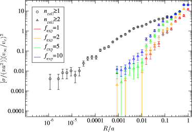
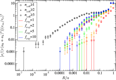
Figure 9: Normalized cross section for physical collisions in binary–single (left) and binary–binary (right) scattering as a function of the ratio of each star’s radius to each binary’s semimajor axis, $R/a$, for different values of the expansion parameter, $f_{\rm exp}$. Circles represent outcomes with one or more collisions; triangles, two or more; and squares, three or more. Red represents runs with $f_{\rm exp}=1$; orange, $f_{\rm exp}=2$; green, $f_{\rm exp}=5$; and blue, $f_{\rm exp}=10$. In both experiments (binary–single and binary–binary), each star had mass $M_{\sun}$ and radius $R$, each binary had semimajor axis $a=1\,\mbox{AU}$ and eccentricity $e=0$, and the relative velocity at infinity was set to $v_{\infty}/v_{c}=0.1$. Calculations were performed down to $R/a=10^{-9}$, but no collisions were found below $R/a\approx 10^{-6}$.

Figure 9 shows the normalized, dimensionless collision cross section, $\sigma(v_{\infty}/v_{c})^{2}/(\pi a^{2})$ for binary–single scattering (left), $\sigma(v_{\infty}/v_{c})^{2}/(\pi(a_{0}+a_{1})^{2})$ for binary–binary scattering (right), as a function of the ratio of stellar radius to binary semimajor axis, $R/a$, for different values of the expansion parameter, $f_{\rm exp}$. Circles represent outcomes with one or more collisions; triangles, two or more; and squares, three or more. Red represents runs with $f_{\rm exp}=1$; orange, $f_{\rm exp}=2$; green, $f_{\rm exp}=5$; and blue, $f_{\rm exp}=10$. In both experiments (binary–single and binary–binary), each star had mass $M_{\sun}$ and radius $R$, each binary had semimajor axis $a=1\,\mbox{AU}$ and eccentricity $e=0$, and the relative velocity at infinity was set to $v_{\infty}/v_{c}=0.1$. Calculations were performed down to $R/a=10^{-9}$ – which corresponds to the extreme case of binaries with semimajor axis $10\,\mbox{AU}$ composed of black holes of mass $M_{\sun}$ – but no collisions were found below $R/a\approx 10^{-6}$. For $n_{\rm coll}\geq 1$, the calculation corresponds to the simpler task of recording minimum close approach distances, as can be seen by comparing the binary–binary panel (right) to Figure 6. The $n_{\rm coll}\geq 2$ and $n_{\rm coll}\geq 3$ collision cross sections decrease more sharply than the $n_{\rm coll}\geq 1$ cross section as $R/a$ decreases.

It is clear that multiple collisions are unlikely for $R/a\la 0.001$, which corresponds roughly to stars of radius $R_{\sun}$ in binaries with semimajor axis $1\,\mbox{AU}$. We therefore expect that multiple collisions in binary interactions are relevant only for MS stars in binaries tighter than $\sim 1\,\mbox{AU}$, white dwarfs in binaries tighter than $\sim 1\,R_{\sun}$, and neutron stars in binaries tighter than $\sim 10^{4}\,$km. We caution that relativistic effects may need to be included when considering close approaches of neutron stars. However, the limits quoted should serve as a rough guide.

We have held the stellar masses fixed at $M_{\sun}$, while varying their radii over a large range. For MS stars, it is more realistic to adopt a reasonable mass-radius relationship, which we do in § 6 for several sets of masses.

5.3 Dependence on mass ratio

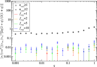
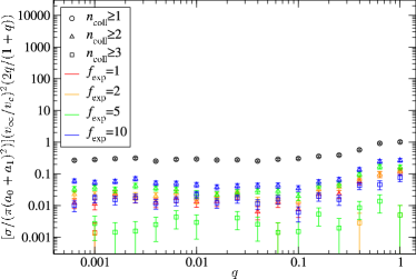
Figure 10: Normalized cross section for physical collisions in binary–single (left) and binary–binary (right) scattering as a function of mass ratio, $q$, for different values of the expansion parameter, $f_{\rm exp}$. Circles represent outcomes with one or more collisions; triangles, two or more; and squares, three or more. Red represents runs with $f_{\rm exp}=1$; orange, $f_{\rm exp}=2$; green, $f_{\rm exp}=5$; and blue, $f_{\rm exp}=10$. In both experiments (binary–single and binary–binary), each binary had one star with mass $M_{\sun}$ and the other with mass $qM_{\sun}$. For the binary–single case, the incoming single star had mass $M_{\sun}$. Each star had radius $R_{\sun}$, each binary had semimajor axis $a=1\,\mbox{AU}$ and eccentricity $e=0$, and the relative velocity at infinity was set to $v_{\infty}/v_{c}=0.1$.

In binary interactions involving stars of different masses, there is a strong tendency for the lightest star(s) to be ejected quickly (see, e.g., Heggie & Hut, 2003). One would expect, then, that resonant behavior, and the likelihood of collisions, would be decreased when one or more of the stars involved are light. To test this prediction, we have calculated the collision cross section during binary–single and binary–binary scattering for a range of mass ratios. In both experiments, each binary had one star with mass $M_{\sun}$ and the other with mass $qM_{\sun}$. For the binary–single case, the incoming single star had mass $M_{\sun}$. Each star had radius $R_{\sun}$, each binary had semimajor axis $a=1\,\mbox{AU}$ and eccentricity $e=0$, and the relative velocity at infinity was set to $v_{\infty}/v_{c}=0.1$. We normalize the cross section, as usual, by multiplying by $(v_{\infty}/v_{c})^{2}$, and, in doing so, inadvertently introduce a dependence on the mass ratio, $q$, in $v_{c}^{2}$. To remove it, we also multiply by a function of $q$ alone that has the same dependence on $q$ as $v_{c}^{2}$, from eqs. (1) and (2), and is normalized to 1 at $q=1$. For binary–single interactions this function is $2q(2+q)/(3(1+q))$; for binary–binary interactions it is $2q/(1+q)$. The collision cross sections are shown in Figure 10 for binary–single (left) and binary–binary (right), as a function of $q$, for different values of the expansion parameter, $f_{\rm exp}$. Circles represent outcomes with one or more collisions; triangles, two or more; and squares, three or more. Red represents runs with $f_{\rm exp}=1$; orange, $f_{\rm exp}=2$; green, $f_{\rm exp}=5$; and blue, $f_{\rm exp}=10$. As expected, the collision cross section is smaller for $q<1$. However, it decreases quickly, and for $q\la 0.1$ becomes approximately constant, implying that the test particle limit has been reached. What is most striking is that the collision cross section is decreased by no more than a factor of a few for small $q$, despite the tendency for lighter stars to be ejected quickly. It should be noted that in this experiment we have kept the radii of all stars fixed at $R_{\sun}$.

6 Results for typical binaries

We now turn from a slicing of parameter space to a discrete sampling, by considering binaries with sets of parameters typical of those found in the cores of globular clusters. We first present results for binary–single interactions, and then binary–binary.

6.1 Binary–single scattering experiments

We consider only MS stars with masses $0.5\,M_{\sun}$, $1.0\,M_{\sun}$, or $1.2\,M_{\sun}$. We adopt the mass-radius relationship $R=R_{\sun}(M/M_{\sun})$, which is a reasonable approximation for MS stars of mass $\sim 1\,M_{\sun}$. We study five different mass combinations, labelled A through E, with a range of semimajor axes, $0.05\,\mbox{AU}\leq a\leq 3.0\,\mbox{AU}$, for each. In all cases we use $v_{\infty}=10\,\mbox{km/s}$. This choice of parameters covers a range of binary binding energies from $\sim 1\,kT$ (the hard-soft boundary) in a typical globular cluster core, to $\sim 10^{2}\,kT$, corresponding to a close binary ($a\sim 10R_{\sun}$). The thermal energy $kT$ is defined by the relation $\frac{1}{2}kT=\frac{1}{2}\langle m\rangle\sigma^{2}$, where $\langle m\rangle$ is the average stellar mass, and $\sigma$ is the one-dimensional velocity dispersion. The details of each run are presented in Table 4, including run name; the number of scattering interactions performed, $N$; the masses of the binary members, $m_{00}$ and $m_{01}$; the mass of the intruder, $m_{1}$; the binary semimajor axis, $a$; and the $n_{\rm coll}\geq 1$ cross section.

In order to study the dependence of the collision cross section on the expansion parameter, $f_{\rm exp}$, without performing calculations for each value of $f_{\rm exp}$ considered, we have adopted an approach that allows us to calculate multiple collision cross sections for any value of $f_{\rm exp}$ based on the results of calculations for one value of $f_{\rm exp}$. We set $f_{\rm exp}=1$, and consider the properties of merger binaries formed. A binary containing a merger product will be a triple-star merger if the pericentre of the binary, $r_{p}$, is approximately less than the radius of the collision product, $R_{\rm cp}=f_{\rm exp}(R_{1}+R_{2})$, where $R_{1}$ and $R_{2}$ are the radii of the two stars that merged to form the collision product. First we calculate $N_{\rm coll}$, the total number of outcomes that resulted in either merger binaries or triple mergers with $f_{\rm exp}=1$. We then calculate $N_{\rm 3coll}$, the number of triple mergers, for a different value of $f_{\rm exp}$, as the number of triple mergers for $f_{\rm exp}=1$, plus the number of merger binaries with $r_{p}<R_{\rm cp}$. Defining $f_{T}=N_{\rm 3coll}/N_{\rm coll}$, the triple-star merger ($n_{\rm coll}\geq 2$) cross section for $f_{\rm exp}$ is simply $\sigma_{T}(f_{\rm exp})=f_{T}\sigma_{\rm coll}(f_{\rm exp}=1)$.

Some remarks about this approach are in order. We ignore merger escapes, and argue that an outcome labelled as a merger escape is unlikely to become a triple merger even if the first merger product expands. Before it escapes, the third star can approach the expanded merger at most once, and, if it does, it is likely to have a sufficiently high speed at close approach to fully traverse the tenuous envelope of the expanded merger product. On the contrary, in a merger binary, even if the third star initially has a high pericentric speed, it will eventually be captured through gradual energy loss after repeated traversal. Of course, an escaping third star may lose sufficient energy after traversal so that the entire system becomes bound, and eventually be captured. A more precise treatment would be to run calculations for each value of $f_{\rm exp}$, but, as mentioned above, we are adopting the simpler, less computationally expensive approach here. When two MS stars collide and their merger product expands, the resulting object does not possess a well-defined boundary and, in general, is not spherically symmetric; $f_{\rm exp}$ is thus an effective, averaged quantity, which serves well enough the purpose of our first study.

6.1.1 Collision cross sections

The $n_{\rm coll}\geq 1$ cross sections are listed in the last column of Table 4. The cross sections from runs A, B, and C are also shown as a function of the initial binary semimajor axis, $a$, in Figure 11. In the range of MS masses of interest for globular clusters, the collision cross sections show only a weak dependence on masses, slightly more pronounced at small $a$. The cross section increases from case A to C as the mass ratios of the stars decrease, due to the dependence of the normalized cross section on $v_{\infty}/v_{c}$ and hence on the mass ratio. For a hard binary with $a\sim 1\,\mbox{AU}$, the normalized collision cross section is comparable to the geometric cross section of the initial binary (i.e., $\sigma_{\rm coll}(v_{\infty}/v_{c})^{2}\sim\pi a^{2}$). This is because most strong interactions are resonant, and most resonances lead to at least one collision. For $a\la 0.1\,\mbox{AU}$, the collision cross section can be up to an order of magnitude greater than the geometric cross section. Indeed, for very small values of $a$, even a small perturbation of a highly eccentric orbit by a distant encounter can induce a binary merger. About 20 to 35% of the initial binaries with $a=0.05\,\mbox{AU}$ in Table 4 have pericentre distances less than $3\,R_{\sun}$. Our results for these very tight binaries are therefore somewhat artificial, since in reality tidal circularization effects are likely to modify the distribution of initial eccentricities, and our simple assumption of a thermal initial distribution is no longer justified.

6.1.2 Properties of the merger binaries

Of particular interest are binary–single interactions that result in binaries containing merger products. The distributions of their properties are relevant to observations of BSs in the cores of globular clusters. Figures 12 and 13 show the orbital parameters of the merger binaries produced in the two representative runs A300, for a wide initial binary, and B005, for a very tight initial binary. The envelope of the distribution follows curves of constant angular momentum, consistent with angular momentum conservation during the interaction. The total angular momentum of the system is the sum of the initial internal angular momentum of the binary and the initial angular momentum of the binary–single hyperbolic orbit, added vectorially. The spread in angular momentum spanned by the distributions is due to averaging over the relative orientation of the two separate angular momenta, the range of initial eccentricities of the binary, and range of impact parameters used. Curves of constant angular momentum are plotted in Figure 12, for the values $J/J_{0}=0.2$, 0.5, 1.0, and 2.0, where $J_{0}=\mu bv_{\infty}+\mu_{b}[GM_{b}a(1-e^{2})]^{1/2}$ is the angular momentum of the system such that the pericentre distance of the initial hyperbolic orbit is $1.0\,\mbox{AU}$ (i.e., $b=r_{p}(1+2GM/r_{p}v_{\infty}^{2})^{1/2}$ with $r_{p}=1.0\,\mbox{AU}$). (Here $\mu$ and $M$ are the reduced and total mass of the binary–single system, and $\mu_{b}$ and $M_{b}$ are the reduced and total mass of the binary.) The vertical dashed line in Figures 12 and 13 is the hard-soft boundary with respect to field stars of mass $1\,M_{\sun}$ with one-dimensional velocity dispersion $10\,\mbox{km/s}$. Histograms of final semi-major axes and eccentricities are shown in Figures 14 and 15. The dotted lines in Figure 15 are properly normalized thermal eccentricity distributions.

Typically, more than 90% of the merger binaries have final semimajor axis, $a^{\prime}$, larger than initial, $a$. On average, $a^{\prime}/a\approx 5$. While most remain hard binaries, a small fraction become soft, with a few having $a^{\prime}$ as large as $\sim 100-1000\,\mbox{AU}$. This softening comes from the somewhat counter-intuitive result that collisions produce, on average, an increase in the orbital energy of the system (while the total energy, including the binding energy of the collision product, is of course conserved on a dynamical time-scale, i.e., until some of the internal energy released through shocks can be radiated away by the fluid). To illustrate this, consider a trivial example in which two identical stars of mass $m$ are released from rest at some distance $r$ and collide head-on, forming a stationary merger product at the centre of mass. The orbital energy of the system increased by $Gm^{2}/r$ in the process. More relevant to our results, but still somewhat artificial, consider an initial binary with a very high eccentricity, so that the two members almost collide at pericentre. A small perturbation through a distant encounter can induce a merger of the binary (implying that its orbital binding energy disappears), while only weakly affecting the orbit of the perturber.

The eccentricity distributions of merger binaries always remain close to thermal, although a slight excess of highly eccentric orbits is seen for wider initial separations (compare run A300, with $a=3\,\mbox{AU}$, and B005, with $a=0.05\,\mbox{AU}$, in Figure 15). The average value of $e^{\prime}$ for runs A300 and B005 is $0.77$ and $0.68$, respectively, while that of a thermal distribution is $2/3$. It is interesting to note that other calculations of small-$N$ systems have yielded binaries with an excess of high eccentricity systems in a nearly thermal distribution (Portegies Zwart & McMillan, 2000).

6.1.3 Three-star mergers

Three-star mergers happen primarily when the pericentre distance of a merger binary is approximately smaller than the radius of the merger remnant. Cumulative distributions of pericentre distances from all A runs are shown in Figure 16. For radii of first collision products in the range $\sim 5$–$10\,R_{\sun}$ ($f_{\rm exp}\sim 2.5$–$5$), we find triple collision fractions anywhere from a few percent up to 50%, depending strongly on the initial binary semi-major axis $a$. Clearly, triple collisions occur often, particularly during encounters with very hard binaries. If we consider the later expansion of the collision product on the giant branch (with radius up to $\ga 100\,\mbox{AU}$), a triple collision becomes almost inevitable, except for only the widest initial binaries.

Denoting the value of $R_{\rm cp}$ at which $f_{T}=f$ by $R_{f}$, we determine the critical radii of merger products corresponding to a given triple collision fraction, $R_{0.05}$, $R_{0.1}$, $R_{0.5}$, $R_{0.9}$ and $R_{0.95}$, using simple linear interpolation. These are plotted as a function of the initial binary separation $a$ in Figure 17. The error bars in Figure 17 are estimated by dividing the uncertainty in $f_{T}$ by the slope of the $f_{T}$ vs $R_{\rm cp}$ curve at $R_{\rm cp}=R_{f}$, i.e.,

$$\Delta R_{f}\simeq\frac{\sqrt{f/N_{\rm coll}}}{(df/dR_{\rm cp})_{R_{f}}}\,.$$ (8)

We see that all the lines in Figure 17 are nearly parallel and with a slope close to unity. The same holds true for mass combinations B through E as well. Thus we have approximately $R_{f}\propto a$ and the relationship can be specified by a single quantity $R_{f}/a$ for each value of $f_{T}$. These have been estimated using a least-squares fit with weights inversely proportional to the size of the error bars. Since hydrodynamic calculations have shown that $R_{\rm cp}$ is unlikely to be larger than $\sim 30$ times the original stellar radius, according to Figure 17, the most relevant range corresponds to $f_{T}\la 0.5$ (although the full range up to $f_{T}\approx 1$ will be relevant if the later expansion of the merger product on the red giant branch is considered). In Figure 18 we plot $R_{f}/a$ as a function of $f_{T}$. It is clear that $R_{f}/a$ is directly proportional to $f_{T}$ over the range of interest. For run A (equal mass case), the proportionality constant is $1.61\pm 0.01$. Consequently, the relation between $R_{\rm cp}$, $f_{T}$ and $a$ for this particular mass combination may be written

$$R_{\rm cp}\approx 1.6af_{T}\,,$$ (9)

where $0.05\,\mbox{AU}\leq a\leq 3.0\,\mbox{AU}$. Turning to different mass combinations we find results similar to eq. (9), and so can write

$$R_{\rm cp}=Caf_{T}\,,$$ (10)

where $C$ depends only on the stellar masses. Table 5 shows $C$ for the five mass combinations we have explored.

6.2 Binary–binary scattering experiments

For the sake of convenience, we use the abbreviations listed in Table 2 to refer to certain binary–binary outcomes. In the abbreviated form, the letters S, D, T, and Q denote a single star, double-star merger, triple-star merger, and quadruple-star merger, respectively, and we have also chosen to use parentheses instead of square brackets. Each run we do involves MS stars of either $0.5\,M_{\sun}$ or $1.0\,M_{\sun}$ and binary semimajor axes of either $1.0\,\mbox{AU}$ or $0.1\,\mbox{AU}$. In all runs we set $v_{\infty}=10\,\mbox{km/s}$, as in the binary–single case. The properties of each run are listed in Table 6, including the mass of each star, $m_{ij}$, the semimajor axis of each binary, $a$, and the normalized cross sections for strong interactions and at least one collision to occur.

To study the dependence of the outcomes on the expansion parameter, $f_{\rm exp}$, we have performed separate calculations for each value of $f_{\rm exp}$ considered. For binary–binary interactions, the dynamics do not reduce to the trivial analytical case of two-body motion after one collision has occurred, and so it is not possible to use the simple approach of tracking pericentre distances in merger binaries as we did for the binary–single case. It should be noted, however, that we apply the simple expansion factor prescription for the radius of a merger product, $R_{\rm merger}=f_{\rm exp}(R_{1}+R_{2})$, where $R_{1}$ and $R_{2}$ are the radii of the merging stars, to every merger, regardless of whether the merging stars are unperturbed MS stars or merger products themselves. The simplicity of this prescription allows us to study the dependence of our results on only one parameter, $f_{\rm exp}$, which can thus be considered an effective expansion parameter, averaged over all types of mergers. A more realistic approach that adopts separate expansion parameters for different types of mergers is feasible, but beyond the scope of this study.

6.2.1 Collision cross sections

The normalized cross sections for strong interactions, $\sigma_{\rm strong}$, and for at least one collision, $\sigma_{\rm coll}$, for our binary–binary runs are listed in the last two columns of Table 6. A strong interaction is defined to be one in which the final configuration is different from the initial configuration (i.e., anything but preservation), or a preservation resulting from a resonant encounter. The test for a resonant encounter is that of Hut & Bahcall (1983), wherein the mean square distance between pairs of stars is checked for multiple minima.

Comparing the results from run I ($a_{0}=a_{1}=1\,\mbox{AU}$) with run II ($a_{0}=a_{1}=0.1\,\mbox{AU}$), we see that $\sigma_{\rm coll}$ is a larger fraction of $\sigma_{\rm strong}$ for run II, consistent with our findings in § 5.2 for small $R/a$. Comparing run II with run IV, we see that introducing a non-unity mass ratio does not seem to affect $\sigma_{\rm strong}$, but slightly lowers $\sigma_{\rm coll}$. By calculating the branching ratio for outcome X involving collisions – defined as $f_{X}=N_{X}/N_{\rm coll}$ where $N_{\rm coll}$ is the number of outcomes that result in collisions and $N_{X}$ is the number of those that result in outcome X – the value of $\sigma_{\rm coll}$ for a particular run can be used to calculate the cross section for outcome X, according to the simple relation $\sigma_{X}=f_{X}\sigma_{\rm coll}$.

6.2.2 Properties of merger products

In Figures 19 and 20, we show the branching ratios for several outcomes as a function of $f_{\rm exp}$. That is, we plot the fraction of outcomes involving at least one collision that result in various configurations containing double-star, triple-star, and quadruple-star mergers. Figure 19 shows results from run I ($a_{0}=a_{1}=1\,\mbox{AU}$) and Figure 20 shows results from run II ($a_{0}=a_{1}=0.1\,\mbox{AU}$). The upper left panel in each shows the branching ratios for outcomes of two unbound double-star mergers, labelled DD, and two double-star mergers in a binary, labelled (DD); the upper right, a quadruple-star merger, labelled Q; the lower right, a triple-star merger bound to the remaining single star, labelled (TS); and the lower left, the combined branching ratio for any outcome involving a merger of three or more stars, labelled T/Q.

From Figure 19, we see that, even for encounters involving wider binaries, the branching ratio for more than two stars to merge is significant – as high as $\sim 5\%$. When one considers tighter binaries, as in Figure 20, the branching ratio increases to $\sim 40\%$. The dependence on initial semimajor axis is as expected – all branching ratios for mergers are increased in run II over run I. The dependence on $f_{\rm exp}$ is also as expected. As the expansion factor is increased, more multiple mergers occur, leading to an increase in the branching ratios for triple-star and quadruple-star mergers, and a decrease in those for double-star mergers.

The distributions of orbital parameters for all four types of binaries, (DS)S, D(SS), (DD), and (TS) are plotted in Figures 21 and 22 for runs I and II, with $f_{\rm exp}=5$. From these figures, we see that (DS) binaries form with semimajor axes comparable to, and only slightly greater than, the semimajor axes of their progenitor binaries (except for the case (DS)S, where $a^{\prime}$ can be significantly larger than $a$ for large $e^{\prime}$), and with an eccentricity distribution that does not appear to be inconsistent with thermal. The data are more sparse for the (DD) and (TS) cases, but their orbital parameters appear to be comparable to those of (DS) binaries.

The three outcomes TS, (TS), and Q (labelled T/Q collectively in Figures 19 and 20), are responsible for the production of BSs of mass $>2M_{\sun}$ in our runs. The branching ratio for T/Q appears to increase almost linearly with $f_{\rm exp}$ in the range considered, for all runs performed. Linear fits for the branching ratio of T/Q as a function of $f_{\rm exp}$ (obtained by least squares fitting) are provided in Table 7.

7 Summary, conclusions, and future directions

We have performed several sets of binary–single and binary–binary scattering experiments, and studied the likelihood of (multiple) collisions. We have presented collision cross sections, branching ratios, and sample distributions of the parameters of outcome products. Results reported in this paper, particularly cross sections, may be employed in both analytical and numerical calculations.

In the gravitational focusing regime, relevant to hard binaries in globular cluster cores, the likelihood of collisions during binary interactions is quite high. For solar mass main-sequence (MS) stars in $1\,\mbox{AU}$ binaries, the normalized cross section for at least one collision to occur during a binary–single or binary–binary interaction ($n_{\rm coll}\geq 1$) is essentially unity, with $\sigma(v_{\infty}/v_{c})^{2}/(\pi a^{2})\sim 1$ for binary–single and $\sigma(v_{\infty}/v_{c})^{2}/(\pi(a_{0}+a_{1})^{2})\sim 1$ for binary–binary. The collision cross section depends strongly on the ratio of stellar radius to binary semimajor axis, but is reasonably high even for MS stars of approximately solar mass in orbits of $\sim 1\,\mbox{AU}$. Perhaps counter to intuition, the collision cross section is not particularly sensitive to binary mass ratio, dropping by only a factor of a few in the test-particle limit when the stellar radii are kept fixed. We also found that the multiple collision ($n_{\rm coll}\geq 2$) cross section is quite high, only a factor of $\sim 10$ lower than the $n_{\rm coll}\geq 1$ cross section for binary–binary interactions. It is also not a particularly sensitive function of the expansion parameter, $f_{\rm exp}$, varying by a factor of a few as $f_{\rm exp}$ is varied by an order of magnitude. This implies that studies using this one-parameter model for the radius of a collision product are reasonably robust in spite of the large uncertainties in the physics. For typical binaries in globular cluster cores, we have shown that collisions of more than two stars during binary–single and binary–binary interactions are likely, with branching ratios for triple-star mergers of $\sim 5\%$ for binary–single and $\sim 10\%$ for binary–binary.

We have introduced Fewbody, a new numerical toolkit for simulating small-$N$ gravitational dynamics that is particularly suited to performing scattering interactions. We have shown that it produces results in good agreement with several previous numerical studies of binary–single and binary–binary scattering, as well as with the Starlab software suite. Instead of using cross sections and simple recipes for binary interactions in globular cluster evolution codes, one may use Fewbody to perform them directly. We have adopted this approach with our Monte Carlo globular cluster evolution code (Fregeau et al., 2003).

It is clear from our results that collisions of more than two stars during binary interactions are a viable pathway for creating blue stragglers (BSs) with masses more than twice the MS turnoff mass, such as those observed in NGC 6397 (Sepinsky et al., 2000). These massive BSs may also be formed via recycling – in other words, a binary containing a BS may be formed via a binary interaction, and the BS may later merge with another star in a subsequent binary interaction, creating a more massive BS. We are in the process of creating a more detailed model, based on a Monte Carlo binary population study, which incorporates both channels to study the formation of massive BSs. Such studies are needed to help interpret current BS observations (see Sills & Bailyn, 1999; Sills et al., 2000), and the large databases of BS properties, including many new spectroscopic mass measurements, that will soon be available (M. Shara, private communication).

The expansion of merger products has been treated here in a simplified manner, using a single expansion parameter, $f_{\rm exp}$. As observations of BSs become more detailed and more numerous, including details of their internal properties, it becomes necessary to treat collisions in a more accurate way. Full smoothed particle hydrodynamics (SPH) calculations are quite computationally prohibitive, taking up to several hours to perform a single merger. However, there are faster, approximate approaches that capture the essential physics of the hydrodynamic merger process. One such approach is the fluid-sorting algorithm, which utilises the property that the fluid in merger products must rearrange itself according to specific entropy (Lombardi et al., 1995, 2002). The Make Me A Star (MMAS) software developed by Lombardi and collaborators implements this procedure, and is freely available on the web (Lombardi et al., 1996, 2002, 2003). We have begun to replace the simple merger module in Fewbody with a call to MMAS. The result should be much more accurate predictions for the properties of (multiple) merger products.

Table 1: Possible outcomes of binary–single star encounters, ordered by the number of collisions, $n_{\rm coll}$. Brackets enclose two objects which are bound to each other, while colons represent physical collisions. For simplicity, we have only listed the outcomes that would result from indistinguishable stars.

$n_{\rm coll}$	symbol	description
0	[$\bullet$ $\bullet$] $\bullet$	preservation or exchange
0	$\bullet$ $\bullet$ $\bullet$	ionization
0	[[$\bullet$ $\bullet$] $\bullet$]	stable hierarchical triple
1	[$\bullet$:$\bullet$ $\bullet$]	binary containing a two-star merger
1	$\bullet$:$\bullet$ $\bullet$	two-star merger and single star
2	$\bullet$:$\bullet$:$\bullet$	three-star merger

Table 2: Possible outcomes of binary–binary star encounters, ordered by the number of collisions, $n_{\rm coll}$. Brackets enclose two objects which are bound to each other, while colons represent physical collisions. For simplicity, we have only listed the outcomes that would result from indistinguishable stars. Listed in the third column are the abbreviations used in the paper to refer to various outcomes.

$n_{\rm coll}$	symbol	abbreviation	description
0	[$\bullet$ $\bullet$] [$\bullet$ $\bullet$]		preservation or exchange
0	[$\bullet$ $\bullet$] $\bullet$ $\bullet$		single ionization
0	$\bullet$ $\bullet$ $\bullet$ $\bullet$		full ionization
0	[[$\bullet$ $\bullet$] $\bullet$] $\bullet$		stable hierarchical triple and single star
0	[[[$\bullet$ $\bullet$] $\bullet$] $\bullet$]		stable hierarchical quadruple
0	[[$\bullet$ $\bullet$] [$\bullet$ $\bullet$]]		stable quadruple composed of two binaries
1	[$\bullet$ $\bullet$] $\bullet$:$\bullet$	(SS)D	binary and two-star merger
1	[$\bullet$:$\bullet$ $\bullet$] $\bullet$	(DS)S	single star and binary containing two-star merger
1	$\bullet$:$\bullet$ $\bullet$ $\bullet$	DSS	two-star merger and two single stars
1	[[$\bullet$:$\bullet$ $\bullet$] $\bullet$]	((DS)S)	stable hierarchical triple with two-star merger in inner binary
1	[[$\bullet$ $\bullet$] $\bullet$:$\bullet$]	((SS)D)	stable hierarchical triple with two-star merger in outer binary
2	[$\bullet$:$\bullet$ $\bullet$:$\bullet$]	(DD)	binary composed of two two-star mergers
2	[$\bullet$:$\bullet$:$\bullet$ $\bullet$]	(TS)	binary containing a three-star merger
2	$\bullet$:$\bullet$ $\bullet$:$\bullet$	DD	two two-star mergers
2	$\bullet$:$\bullet$:$\bullet$ $\bullet$	TS	three-star merger and single star
3	$\bullet$:$\bullet$:$\bullet$:$\bullet$	Q	four-star merger

[levelsep=40pt]0  [levelsep=40pt]1  [levelsep=40pt]2  [levelsep=40pt]3  $\cdots$  [levelsep=40pt]$N$

Figure 1: Schematic representation of the binary-tree algorithm used by Fewbody. A circle containing a number represents a star. The set of binary trees is shown flattened here, as it is before processing, so that each star is the top-level node of a one-node tree.

[levelsep=40pt]0  [levelsep=40pt]0 1 2  [levelsep=40pt]3  $\cdots$  [levelsep=40pt]$N$

Figure 2: Schematic representation of the binary-tree algorithm used by Fewbody. A circle containing a number represents a star, while an empty circle represents a general parent node. The set of binary trees is shown after the first stage of processing, with stars 1 and 2 replaced by their parent node, which contains the dynamical information pertaining to the centre of mass of the 1-2 binary, as well as all phase and orientation information. For classification, the replacement of stars 1 and 2 by their parent node simply means that they are bound to each other with the smallest semimajor axis. For hierarchy isolation, it would also mean that the 1-2 binary is sufficiently weakly perturbed that it can be treated analytically, and is stable in the sense that its two members will not collide at pericentre.

[levelsep=40pt]0  [levelsep=40pt]0 [levelsep=40pt]012 3  $\cdots$  [levelsep=40pt]$N$

Figure 3: Schematic representation of the binary-tree algorithm used by Fewbody. A circle containing a number represents a star, while an empty circle represents a general parent node. The set of binary trees is shown after the second stage of processing, with the 1-2 centre of mass and star 3 replaced by their parent node. For hierarchy isolation, this replacement is quite rare, as it would require that the triple be not only dynamically stable, but also sufficiently hierarchical that its evolution could be treated analytically.

Table 3: Comparison of Fewbody with Table 5 of Mikkola (1983a): fraction of strong binary–binary interactions that result in various outcomes. In each binary–binary interaction the stars had equal masses and were assumed to be point particles, the binaries had equal semimajor axes, and the eccentricities were drawn from a thermal distribution. The data are normalized to 100 total scattering experiments. The results are also shown graphically in Figure 5.

$v_{\infty}/v_{c}$	method	undecided	exchange	triple	single ionization	full ionization	total
$0.316$	Mikkola	$4.7\pm 1.2$	$11.0\pm 1.9$	$24.3\pm 2.8$	$60.0\pm 4.5$	$0.0\pm 0.0$	300
	Fewbody	$1.6\pm 0.2$	$6.0\pm 0.3$	$22.8\pm 0.7$	$69.7\pm 1.2$	$0.0\pm 0.0$	5225
$0.500$	Mikkola	$2.7\pm 0.9$	$7.3\pm 1.6$	$20.3\pm 2.6$	$69.7\pm 4.8$	$0.0\pm 0.0$	300
	Fewbody	$1.4\pm 0.2$	$6.7\pm 0.4$	$17.2\pm 0.6$	$74.7\pm 1.3$	$0.0\pm 0.0$	4366
$0.707$	Mikkola	$0.7\pm 0.5$	$9.3\pm 1.8$	$11.7\pm 2.0$	$78.3\pm 5.1$	$0.0\pm 0.0$	300
	Fewbody	$0.5\pm 0.1$	$7.7\pm 0.5$	$6.8\pm 0.5$	$85.0\pm 1.6$	$0.0\pm 0.0$	3303
$0.866$	Mikkola	$0.7\pm 0.5$	$16.7\pm 2.4$	$5.0\pm 1.3$	$77.7\pm 5.1$	$0.0\pm 0.0$	300
	Fewbody	$0.1\pm 0.1$	$8.2\pm 0.5$	$2.3\pm 0.2$	$89.4\pm 1.5$	$0.0\pm 0.0$	3827
$1.000$	Mikkola	$0.0\pm 0.0$	$9.3\pm 1.8$	$1.7\pm 0.7$	$89.0\pm 5.4$	$0.0\pm 0.0$	300
	Fewbody	$0.1\pm 0.0$	$6.4\pm 0.4$	$0.6\pm 0.1$	$92.7\pm 1.6$	$0.2\pm 0.1$	3499
$1.225$	Mikkola	$0.0\pm 0.0$	$8.3\pm 1.7$	$0.7\pm 0.5$	$73.7\pm 5.0$	$17.3\pm 2.4$	300
	Fewbody	$0.0\pm 0.0$	$4.6\pm 0.3$	$0.2\pm 0.1$	$92.1\pm 1.5$	$3.1\pm 0.3$	3969

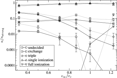
Figure 5: Comparison of Fewbody (solid lines) with Table 5 of Mikkola (1983a) (dotted lines): fraction of strong binary–binary interactions that result in various outcomes. In each binary–binary interaction the stars had equal masses and were assumed to be point particles, the binaries had equal semimajor axes, and the eccentricities were drawn from a thermal distribution. Circles represent outcomes that were undecided after a preset maximum computation time, squares represent exchanges, diamonds represent stable hierarchical triples, upward-pointing triangles represent outcomes that resulted in one binary being disrupted, and downward-pointing triangles represent outcomes that resulted in both binaries being disrupted. The solid lines represent Fewbody data, while the dotted lines represent data from Mikkola (1983a). The results are also presented in Table 3.

Figure 6: Comparison of Fewbody with Figure 4 of Bacon et al. (1996): cumulative cross section for the distance of closest approach in binary–binary scattering for the equal-mass, zero-eccentricity, equal-semimajor-axis case. The stars are assumed to be point particles and $v_{\infty}/v_{c}=0.25$. A total of $1.5\times 10^{4}$ scattering experiments were used to create this figure. The broken power-law is the best fit given by Bacon et al. (1996) to their original results, while the dot-dash curve is Sigurdsson’s recalculation. The dashed curve shows the results obtained using Starlab. There is a clear discrepancy between Fewbody and Bacon et al. (1996), and even the recalculation. However, Fewbody and Starlab agree quite well.

Figure 7: Comparison between scatter3, Starlab’s three-body scattering routine (solid line), and scatter, its $N$-body scattering routine (dashed line). Plotted is the cumulative fraction of binaries as a function of $r_{p}/a$, where $r_{p}$ is the pericentre distance of the merger binary, and $a$ is the initial binary semimajor axis. For the binary–single runs, each star had mass $M_{\sun}$, radius $R_{\sun}$, the binary had semimajor axis $1\,\mbox{AU}$ and $e=0$, and $v_{\infty}=10\,\mbox{km/s}$. In the binary–binary runs, the binary representing the single star had a secondary of mass $10^{-5}\,M_{\sun}$, semimajor axis of $20\,\mbox{AU}$, and $e=0$. The agreement between the two methods is excellent, and in either case, $r_{p}$ is strongly concentrated between $0.15\,\mbox{AU}$ and $0.3\,\mbox{AU}$.

Table 4: Parameters of the binary–single runs, including the number of scattering interactions performed, $N$; the masses of the binary members, $m_{00}$ and $m_{01}$; the mass of the intruder, $m_{1}$; the binary semimajor axis, $a$; and the $n_{\rm coll}\geq 1$ cross section.

run	$N$	$m_{00}\,(M_{\sun})$	$m_{01}\,(M_{\sun})$	$m_{1}\,(M_{\sun})$	$a\,(\mbox{AU})$	$\displaystyle\frac{\sigma_{n_{\rm coll}\geq 1}}{\pi a^{2}}\left(\frac{v_{\infty}}{v_{c}}\right)^{2}$
A005	15054	1.0	1.0	1.0	0.05	$6.4\pm 0.1$
A010	30228	1.0	1.0	1.0	0.1	$5.72\pm 0.07$
A020	15222	1.0	1.0	1.0	0.2	$4.41\pm 0.08$
A050	18158	1.0	1.0	1.0	0.5	$2.87\pm 0.07$
A100	37625	1.0	1.0	1.0	1.0	$1.94\pm 0.04$
A300	21427	1.0	1.0	1.0	3.0	$0.68\pm 0.04$
B005	17619	1.0	0.5	1.0	0.05	$9.3\pm 0.2$
B010	30408	1.0	0.5	1.0	0.1	$7.3\pm 0.1$
B020	17969	1.0	0.5	1.0	0.2	$5.4\pm 0.1$
B050	18676	1.0	0.5	1.0	0.5	$3.0\pm 0.1$
B100	39739	1.0	0.5	1.0	1.0	$1.62\pm 0.05$
B300	28544	1.0	0.5	1.0	3.0	$0.54\pm 0.05$
C005	17696	0.5	0.5	1.0	0.05	$12\pm 2$
C010	35791	0.5	0.5	1.0	0.1	$9.3\pm 0.1$
C020	18284	0.5	0.5	1.0	0.2	$6.6\pm 0.2$
C050	19467	0.5	0.5	1.0	0.5	$3.3\pm 0.1$
C100	49032	0.5	0.5	1.0	1.0	$1.96\pm 0.07$
C300	33464	0.5	0.5	1.0	3.0	$0.58\pm 0.07$
D005	12530	1.0	1.0	0.5	0.05	$2.5\pm 0.1$
D010	12555	1.0	1.0	0.5	0.1	$2.2\pm 0.1$
D020	12610	1.0	1.0	0.5	0.2	$1.75\pm 0.1$
D050	12780	1.0	1.0	0.5	0.5	$1.16\pm 0.08$
D100	15672	1.0	1.0	0.5	1.0	$0.73\pm 0.07$
D300	14185	1.0	1.0	0.5	3.0	$0.26\pm 0.04$
E005	60252	1.0	1.0	1.2	0.05	$8.0\pm 0.2$
E010	60504	1.0	1.0	1.2	0.1	$6.9\pm 0.2$
E020	61008	1.0	1.0	1.2	0.2	$5.4\pm 0.2$
E050	72947	1.0	1.0	1.2	0.5	$3.5\pm 0.1$
E100	75894	1.0	1.0	1.2	1.0	$2.2\pm 0.1$
E300	100200	1.0	1.0	1.2	3.0	$0.80\pm 0.05$

Figure 11: The normalized $n_{\rm coll}\geq 1$ cross section as a function of initial semimajor axis for runs A, B and C.

Figure 12: Distribution of the semimajor axes and eccentricities of the $\sim 700$ merger binaries formed in run A300. The vertical dashed line is the hard-soft boundary for field stars of mass $1.0\,M_{\sun}$ with one-dimensional velocity dispersion $10\,\mbox{km/s}$. The solid curves represent constant angular momenta $J/J_{0}=0.2$, 0.5, 1.0, and 2.0, where $J_{0}$ is the total angular momentum of the system such that the pericentre of the initial hyperbolic orbit is $1.0\,\mbox{AU}$.

Figure 13: Distribution of the semimajor axes and eccentricities of the $\sim 6000$ merger binaries formed in run B005. The vertical dashed line is the hard-soft boundary for field stars of mass $1.0M_{\sun}$ with one-dimensional velocity dispersion $10\,\mbox{km/s}$.

Figure 14: Histograms of semimajor axes of the merger binaries formed in runs A300 and B005, relative to the initial binary semimajor axis.

Figure 15: Histograms of eccentricities of the merger binaries formed in runs A300 and B005. The dotted lines represent properly normalized thermal distributions.

Figure 16: Cumulative distribution of pericentre distance for the merger binaries formed in case A. The dashed lines, from left to right, correspond to $a=0.05$, 0.1, 0.2, 0.5, 1.0 and $3.0\,AU$ respectively. Each curve is equivalent to $f_{T}(R_{\rm cp})$, the fraction of triple mergers as a function of the effective expanded radius of the first collision product, for a given $a$.

Figure 17: $R_{0.95},R_{0.9},R_{0.5},R_{0.1}$ and $R_{0.05}$ as a function of $a$ for case A, where $R_{f}$ is the value of $R_{\rm cp}$ at which $f_{T}=f$.

Figure 18: Dependence of $R_{f}/a$ on $f=f_{T}$, with $f\leq 0.5$, for three different mass combinations. Solid triangles, open squares, and open triangles correspond to cases A, B, and C, respectively.

Table 5: Fits for $C$ in eq.(10) for the different mass combinations considered.

Case	$m_{00}\,(M_{\sun})$	$m_{01}\,(M_{\sun})$	$m_{1}\,(M_{\sun})$	$C$
A	1.0	1.0	1.0	1.61$\pm$0.01
B	1.0	0.5	1.0	1.99$\pm$0.01
C	0.5	0.5	1.0	2.40$\pm$0.02
D	1.0	1.0	0.5	1.64$\pm$0.02
E	1.0	1.0	1.2	1.78$\pm$0.02

Table 6: Parameters of the binary–binary scattering experiments, including the mass of each star, $m_{ij}$, the semimajor axis of each binary, $a_{i}$, and the normalized cross sections for strong interactions and at least one collision to occur.

run	$m_{00}\,(M_{\sun})$	$m_{01}\,(M_{\sun})$	$m_{10}\,(M_{\sun})$	$m_{11}\,(M_{\sun})$	$a_{0}\,(\mbox{AU})$	$a_{1}\,(\mbox{AU})$	$\displaystyle\frac{\sigma_{\rm strong}}{\pi(a_{0}+a_{1})^{2}}\left(\frac{v_{\infty}}{v_{c}}\right)^{2}$	$\displaystyle\frac{\sigma_{n_{\rm coll}\geq 1}}{\pi(a_{0}+a_{1})^{2}}\left(\frac{v_{\infty}}{v_{c}}\right)^{2}$
I	1.0	1.0	1.0	1.0	1.0	1.0	$0.62\pm 0.13$	$0.12\pm 0.07$
II	1.0	1.0	1.0	1.0	0.1	0.1	$0.09\pm 0.03$	$0.04\pm 0.02$
III	1.0	1.0	1.0	1.0	1.0	0.1	$0.090\pm 0.003$	$0.0020\pm 0.0005$
IV	1.0	0.5	1.0	0.5	0.1	0.1	$0.12\pm 0.03$	$0.0099\pm 0.0004$

Figure 19: Branching ratios for various outcomes involving collisions in run I, as functions of the expansion factor.

Figure 20: Branching ratios for various outcomes involving collisions in run II, as functions of the expansion factor.

Figure 21: Orbital parameters of four kinds of binaries formed in run I, with $f_{\rm exp}=5$.

Figure 22: Orbital parameters of four kinds of binaries formed in run II, with $f_{\rm exp}=5$.

Table 7: Linear fits for the branching ratio of T/Q($>2M_{\sun}$) as a function of $f_{\rm exp}$, where $f_{{\rm T/Q}(>2M_{\odot})}=Af_{\rm exp}+B$. Also shown in the last column is the normalized cross section for the formation of triple-star/quadruple-star mergers with masses $>2M_{\sun}$ for $f_{\rm exp}=5$.

run	$A$	$B$	$\displaystyle\frac{\sigma_{{\rm T/Q}(>2M_{\odot})}(f_{\rm exp}=5)}{\pi(a_{0}+a_{1})^{2}}\left(\frac{v_{\infty}}{v_{c}}\right)^{2}$
I	0.007	0.007	$0.011\pm 0.002$
II	0.0485	0.14	$0.035\pm 0.003$
III	0.0182	0.024	$0.00041\pm 0.00005$
IV	0.0249	0.0616	$0.034\pm 0.006$

References

- Aarseth (2003) Aarseth S. J., 2003, Gravitational N-Body Simulations: Tools and Algorithms. Cambridge University Press
- Albrow et al. (2001) Albrow M. D., Gilliland R. L., Brown T. M., Edmonds P. D., Guhathakurta P., Sarajedini A., 2001, ApJ, 559, 1060
- Bacon et al. (1996) Bacon D., Sigurdsson S., Davies M. B., 1996, MNRAS, 281, 830
- Bailyn & Pinsonneault (1995) Bailyn C. D., Pinsonneault M. H., 1995, ApJ, 439, 705
- Bellazzini et al. (2002) Bellazzini M., Fusi Pecci F., Messineo M., Monaco L., Rood R. T., 2002, AJ, 123, 1509
- Bolton et al. (1999) Bolton A. S., Cool A. M., Anderson J., 1999, Bulletin of the American Astronomical Society, 31, 1483
- Bond & Perry (1971) Bond H. E., Perry C. L., 1971, PASP, 83, 638
- Burgarella et al. (1994) Burgarella D., Paresce F., Meylan G., King I. R., Greenfield P., Baxter D., Jedrzejewski R., Nota A., Albrecht R., Barbieri C., Blades J. C., Boksenberg A., Crane P., Deharveng J. M., Disney M. J., Jakobsen P., Kamperman T. M., Macchetto F., Mackay C. D., Weigelt G., 1994, A&A, 287, 769
- Chenciner & Montgomery (2000) Chenciner A., Montgomery R., 2000, Ann. Math., 152, 881
- Cleary & Monaghan (1990) Cleary P. W., Monaghan J. J., 1990, ApJ, 349, 150
- Cote et al. (1994) Cote P., Welch D. L., Fischer P., Da Costa G. S., Tamblyn P., Seitzer P., Irwin M. J., 1994, ApJS, 90, 83
- Davies & Benz (1995) Davies M. B., Benz W., 1995, MNRAS, 276, 876
- Davies et al. (1993) Davies M. B., Benz W., Hills J. G., 1993, ApJ, 411, 285
- Davies et al. (1994) —, 1994, ApJ, 424, 870
- de Angeli & Piotto (2003) de Angeli F., Piotto G., 2003, in ASP Conf. Ser. 296: New Horizons in Globular Cluster Astronomy, p. 296
- de Marchi & Paresce (1994) de Marchi G., Paresce F., 1994, ApJ, 422, 597
- Ferraro et al. (2004) Ferraro F. R., Beccari G., Rood R. T., Bellazzini M., Sills A., Sabbi E., 2004, ApJ, 603, 127
- Ferraro et al. (1997) Ferraro F. R., Paltrinieri B., Fusi Pecci F., Cacciari C., Dorman B., Rood R. T., Buonanno R., Corsi C. E., Burgarella D., Laget M., 1997, A&A, 324, 915
- Ferraro et al. (1999) Ferraro F. R., Paltrinieri B., Rood R. T., Dorman B., 1999, ApJ, 522, 983
- Ferraro et al. (1993) Ferraro F. R., Pecci F. F., Cacciari C., Corsi C., Buonanno R., Fahlman G. G., Richer H. B., 1993, AJ, 106, 2324
- Ferraro et al. (2003) Ferraro F. R., Sills A., Rood R. T., Paltrinieri B., Buonanno R., 2003, ApJ, 588, 464
- Ford et al. (2000) Ford E. B., Kozinsky B., Rasio F. A., 2000, ApJ, 535, 385
- Fregeau et al. (2003) Fregeau J. M., Gürkan M. A., Joshi K. J., Rasio F. A., 2003, ApJ, 593, 772
- Gao et al. (1991) Gao B., Goodman J., Cohn H., Murphy B., 1991, ApJ, 370, 567
- Giersz & Spurzem (2003) Giersz M., Spurzem R., 2003, MNRAS, 343, 781
- Gilliland et al. (1998) Gilliland R. L., Bono G., Edmonds P. D., Caputo F., Cassisi S., Petro L. D., Saha A., Shara M. M., 1998, ApJ, 507, 818
- Goodman & Hernquist (1991) Goodman J., Hernquist L., 1991, ApJ, 378, 637
- Goodman & Hut (1989) Goodman J., Hut P., 1989, Nature, 339, 40
- Gualandris et al. (2004) Gualandris A., Portegies Zwart S., Eggleton P. P., 2004, MNRAS (in press) (astro-ph/0401451)
- Guhathakurta et al. (1998) Guhathakurta P., Webster Z. T., Yanny B., Schneider D. P., Bahcall J. N., 1998, AJ, 116, 1757
- Guhathakurta et al. (1996) Guhathakurta P., Yanny B., Schneider D. P., Bahcall J. N., 1996, AJ, 111, 267
- Harrington (1974) Harrington R. S., 1974, Celestial Mechanics, 9, 465
- Heggie & Hut (2003) Heggie D., Hut P., 2003, The Gravitational Million-Body Problem: A Multidisciplinary Approach to Star Cluster Dynamics. Cambridge University Press
- Heggie (1974) Heggie D. C., 1974, Celestial Mechanics, 10, 217
- Heggie (2000) —, 2000, MNRAS, 318, L61
- Heggie & Aarseth (1992) Heggie D. C., Aarseth S. J., 1992, MNRAS, 257, 513
- Heggie & Rasio (1996) Heggie D. C., Rasio F. A., 1996, MNRAS, 282, 1064
- Hills (1991) Hills J. G., 1991, AJ, 102, 704
- Hills (1992) —, 1992, AJ, 103, 1955
- Hills & Day (1976) Hills J. G., Day C. A., 1976, Astrophys. Lett., 17, 87
- Hoffer (1983) Hoffer J. B., 1983, AJ, 88, 1420
- Hurley et al. (2001) Hurley J. R., Tout C. A., Aarseth S. J., Pols O. R., 2001, MNRAS, 323, 630
- Hut & Bahcall (1983) Hut P., Bahcall J. N., 1983, ApJ, 268, 319
- Hut & Inagaki (1985) Hut P., Inagaki S., 1985, ApJ, 298, 502
- Hut et al. (1992) Hut P., McMillan S., Goodman J., Mateo M., Phinney E. S., Pryor C., Richer H. B., Verbunt F., Weinberg M., 1992, PASP, 104, 981
- Hut & Verbunt (1983) Hut P., Verbunt F., 1983, Nature, 301, 587
- Ivanova et al. (2004) Ivanova N., Belczynski K., Fregeau J. M., Rasio F. A., 2004, submitted to ApJ (astro-ph/0312497)
- Jahn et al. (1995) Jahn K., Kaluzny J., Rucinski S. M., 1995, A&A, 295, 101
- Jeans (1919) Jeans J. H., 1919, MNRAS, 79, 408
- Kaluzny & Rucinski (1993) Kaluzny J., Rucinski S. M., 1993, MNRAS, 265, 34
- Krolik et al. (1984) Krolik J. H., Meiksin A., Joss P. C., 1984, ApJ, 282, 466
- Leonard (1989) Leonard P. J. T., 1989, AJ, 98, 217
- Leonard & Fahlman (1991) Leonard P. J. T., Fahlman G. G., 1991, AJ, 102, 994
- Livio (1993) Livio M., 1993, in ASP Conf. Ser. 53: Blue Stragglers, p. 3
- Lombardi et al. (1995) Lombardi J. C., Rasio F. A., Shapiro S. L., 1995, ApJ, 445, L117
- Lombardi et al. (1996) —, 1996, ApJ, 468, 797
- Lombardi et al. (2003) Lombardi J. C., Thrall A. P., Deneva J. S., Fleming S. W., Grabowski P. E., 2003, MNRAS, 345, 762
- Lombardi et al. (2002) Lombardi J. C., Warren J. S., Rasio F. A., Sills A., Warren A. R., 2002, ApJ, 568, 939
- Mardling & Aarseth (2001) Mardling R. A., Aarseth S. J., 2001, MNRAS, 321, 398
- Mateo et al. (1990) Mateo M., Harris H. C., Nemec J., Olszewski E. W., 1990, AJ, 100, 469
- McMillan & Hut (1994) McMillan S., Hut P., 1994, ApJ, 427, 793
- McMillan et al. (1990) McMillan S., Hut P., Makino J., 1990, ApJ, 362, 522
- McMillan et al. (1991) —, 1991, ApJ, 372, 111
- McMillan (1986) McMillan S. L. W., 1986, ApJ, 306, 552
- McMillan & Hut (1996) McMillan S. L. W., Hut P., 1996, ApJ, 467, 348
- Mikkola (1983a) Mikkola S., 1983a, MNRAS, 203, 1107
- Mikkola (1983b) —, 1983b, MNRAS, 205, 733
- Mikkola (1984a) —, 1984a, MNRAS, 207, 115
- Mikkola (1984b) —, 1984b, MNRAS, 208, 75
- Mikkola (1985) —, 1985, MNRAS, 215, 171
- Miller & Hamilton (2002) Miller M. C., Hamilton D. P., 2002, ApJ, 576, 894
- Milone & Latham (1994) Milone A. A. E., Latham D. W., 1994, AJ, 108, 1828
- Milone et al. (1992) Milone A. A. E., Latham D. W., Mathieu R. D., Morse J. A., Davis R. J., 1992, in IAU Symp. 151: Evolutionary Processes in Interacting Binary Stars, p. 473
- Montgomery (2001) Montgomery R., 2001, Not. AMS, 48, 471
- Portegies Zwart et al. (1997a) Portegies Zwart S. F., Hut P., McMillan S. L. W., Verbunt F., 1997a, A&A, 328, 143
- Portegies Zwart et al. (1997b) Portegies Zwart S. F., Hut P., Verbunt F., 1997b, A&A, 328, 130
- Portegies Zwart & McMillan (2000) Portegies Zwart S. F., McMillan S. L. W., 2000, ApJ, 528, L17
- Portegies Zwart et al. (2001) Portegies Zwart S. F., McMillan S. L. W., Hut P., Makino J., 2001, MNRAS, 321, 199
- Rasio et al. (2001) Rasio F. A., Fregeau J. M., Joshi K. J., 2001, in ASSL Vol. 264: The Influence of Binaries on Stellar Population Studies, p. 387
- Rasio & Heggie (1995) Rasio F. A., Heggie D. C., 1995, ApJ, 445, L133
- Rubenstein & Bailyn (1997) Rubenstein E. P., Bailyn C. D., 1997, ApJ, 474, 701
- Rucinski (2000) Rucinski S. M., 2000, AJ, 120, 319
- Sandquist et al. (2003) Sandquist E. L., Latham D. W., Shetrone M. D., Milone A. A. E., 2003, AJ, 125, 810
- Sepinsky et al. (2000) Sepinsky J. F., Saffer R. A., Pilman C. S., DeMarchi G., Paresce F., 2000, Bulletin of the American Astronomical Society, 32, 740
- Shara et al. (1997) Shara M. M., Saffer R. A., Livio M., 1997, ApJ, 489, L59
- Sigurdsson et al. (1994) Sigurdsson S., Davies M. B., Bolte M., 1994, ApJ, 431, L115
- Sigurdsson & Phinney (1993) Sigurdsson S., Phinney E. S., 1993, ApJ, 415, 631
- Sigurdsson & Phinney (1995) —, 1995, ApJS, 99, 609
- Sills & Bailyn (1999) Sills A., Bailyn C. D., 1999, ApJ, 513, 428
- Sills et al. (2000) Sills A., Bailyn C. D., Edmonds P. D., Gilliland R. L., 2000, ApJ, 535, 298
- Sosin & King (1995) Sosin C., King I. R., 1995, AJ, 109, 639
- Strom et al. (1971) Strom S. E., Strom K. M., Bregman J. N., 1971, PASP, 83, 768
- Stryker (1993) Stryker L. L., 1993, PASP, 105, 1081
- Yan & Mateo (1994) Yan L., Mateo M., 1994, AJ, 108, 1810
- Yanny et al. (1994a) Yanny B., Guhathakurta P., Bahcall J. N., Schneider D. P., 1994a, AJ, 107, 1745
- Yanny et al. (1994b) Yanny B., Guhathakurta P., Schneider D. P., Bahcall J. N., 1994b, ApJ, 435, L59