XMM-Newton and VLT observations of the isolated neutron star 1E 1207.4–5209 

In August 2002, XMM-Newton devoted two full orbits to the observation of 1E 1207.4–5209 , making this isolated neutron star the most deeply scrutinized galactic target of the mission. Thanks to the high throughput of the EPIC instrument, $\sim$ 360,000 photons were collected from the source, allowing for a very sensitive study of the temporal and spectral behaviour of this object. The spectral data, both time-averaged and phase-resolved, yield one compelling interpretation of the observed features: cyclotron absorption from one fundamental ($\sim 0.7$ keV) and three harmonics, at $\sim 1.4$, $\sim 2.1$ and $\sim 2.8$ keV. Possible physical consequences are discussed, also on the basis of the obvious phase variations of the features’ shapes and depths. We also present deep VLT optical data which we have used to search for a counterpart, with negative results down to $V\sim 27$.

1 Introduction

The X-ray source 1E 1207.4–5209 attracted much interest since its early discovery (Helfand & Becker 1984) as a bright unresolved source located at the geometrical center of the shell-like radio/X-ray/optical supernova remnant G 296.5+10.0  (Roger et al. 1988). X–ray observations with the Einstein (Helfand & Becker 1984), EXOSAT (Kellet et al. 1987), ROSAT (Mereghetti et al. 1996) and ASCA (Vasisht et al. 1997) satellites showed a steady flux of $\sim$2$\times$10^-12 erg cm^-2 s^-1 (0.3-3 keV) characterized by a thermal spectrum. These observations, coupled with the lack of an optical counterpart down to $V\sim 25$ (Bignami et al. 1992; Mereghetti et al. 1996) strongly suggested a neutron star nature for 1E 1207.4–5209 . This hypothesis was later confirmed by the Chandra detection of fast X–ray pulsations with period $P$=0.424 s (Zavlin et al. 2000) and period derivative $\dot{P}$ = (2.0${}^{+1.1}_{-1.3}$) $\times$ 10^-14 s s^-1 (Pavlov et al. 2002).

The Chandra data also unveiled the presence of broad absorption features at energies of $\sim$0.7 and $\sim$1.4 keV (Sanwal et al. 2002). The existence of these features was soonafter confirmed by an XMM-Newton observation, which showed that the depths and profiles of the two lines vary significantly with the rotational phase of the pulsar (Mereghetti et al. 2002a, hereafter Paper I).

Although observationally firmly established, the nature of these lines could not be unambiguously identified. They were attributed either to HeII transitions in a “Magnetar”-like field B$\sim$(1.4–1.7)$\times$10¹⁴ G (Sanwal et al. 2002) or to atomic transitions in heavier elements (e.g. He-like Oxigen or Neon) in the atmosphere of a neutron star with a more conventional magnetic field (Hailey & Mori 2002). An alternative explanation of the lines as cyclotron features was considered to be unlikely by Sanwal et al. (2002). This view was criticized by Xu et al. (2003), who interpreted the lines as electron cyclotron resonance features originating near the neutron star surface.

The breakthrough came with a longer XMM-Newton observation which, besides confirming the two phase-dependent absorption lines at 0.7 and 1.4 keV, showed a statistically significant third line at $\sim$2.1 keV, as well as a hint for a possible fourth feature at 2.8 keV (Bignami et al. 2003, hereafter Paper II). The nearly 1:2:3:4 ratio of the line centroids, as well as the phase variation, naturally following the pulsar B-field rotation, strongly suggest that such lines are due to cyclotron absorption processes in a magnetic field of $\sim$8$\times 10^{10}$ G or $\sim$1.6$\times 10^{14}$ G, respectively in the case of electrons or protons features.

Thus, among known isolated neutron stars, 1E 1207.4–5209 stands out as the only one which clearly exhibits X–ray absorption lines.

Here we present a comprehensive analysis of the data collected during the long XMM-Newton observation, already shortly discussed in Paper II, as well as new optical images of the field, the deepest available so far, performed with the VLT.

2 XMM-Newton Data reduction and analysis

The XMM-Newton observation of 1E 1207.4–5209 started on August 4, 2002 and lasted two full orbits yielding two uninterrupted time intervals of $\sim$36 hours each.

The data reported here were obtained with the European Photon Imaging Camera (EPIC) instrument, which consists of two MOS CCD detectors (Turner et al. 2001) and a pn CCD instrument (Strüder et al. 2001), for a total collecting area $\;\buildrel>\over{\sim}\;$2500 cm² at 1.5 keV. The mirror system offers an on-axis point spread function of 4-5^′′ FWHM and a field of view of 30^′ diameter.

While the two MOS cameras were operated in “full frame” mode, the pn camera was operated in “small window” mode to allow for the accurate timing of the source photons (6 ms resolution). All cameras used the thin filter. The data were processed with the latest release of the XMM Newton Science Analysis Software (SAS version 5.4.1). After screening the data to remove time intervals with high particle background and correcting for the dead time, we obtain a net exposure time of 139.0 ksec for the pn camera and 197.5 and 197.3 ks for the MOS1 and MOS2, respectively.

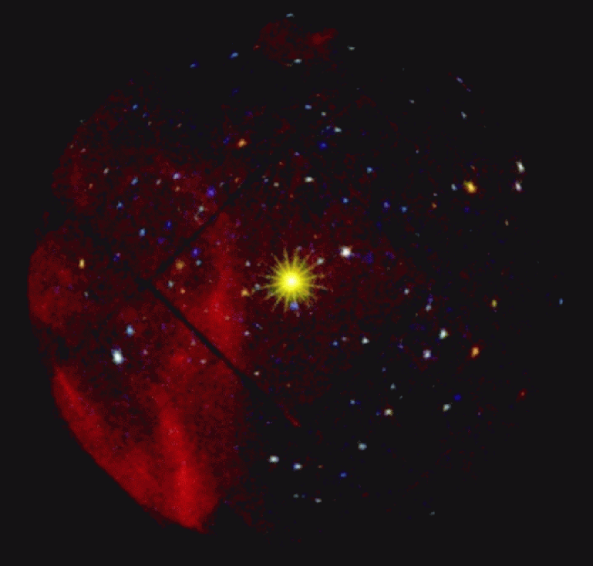
Figure 1: The XMM-Newton view of the field of 1E 1207.4–5209 . Data from the MOS1 and MOS2 camera have been merged to produce the image. The exposure time is of $\sim$200 ksec per camera. The target is the bright source close to the center of the field. Many ($\sim$200) serendipitous sources and the bright emission from parts of the shell of the host supernova remnant G296.5+10.0 are clearly visible. The colors are energy-coded, red represents photons in the 0.3-0.6 keV band, green and blue correspond to the 0.6-1.5 keV and 1.5-8 keV bands respectively

The source 1E 1207.4–5209 is clearly detected in the three EPIC cameras. In the energy range 0.2-5 keV it yields net count rates of 1.466$\pm$0.003 cts s^-1, 0.380$\pm$0.002 cts s^-1 and 0.389$\pm$0.002 cts s^-1 in the pn, MOS1, and MOS2 respectively.

The field of 1E 1207.4–5209 as seen by EPIC is shown in Fig. 1. Data from the MOS1 and MOS2 cameras have been merged to produce the image, which has energy-coded colors (see caption).

In the MOS field of view a large ($\sim 200$) number of serendipitous sources are detected. Bright emission from parts of the surrounding supernova remnant G296.5+10.0 is also visible. No extended emission is seen around 1E 1207.4–5209 or in its immediate vicinity (within $\sim$2 arcmin). The radial intensity profile of the target is fully consistent with the instrumental point spread function (Ghizzardi 2002).

To derive the sky coordinates of 1E 1207.4–5209 we computed the boresight correction to be applied to the default EPIC astrometry. This was done independently for the MOS1 and MOS2 cameras; the pn data were not used since the small field of view (4$\times$4 arcmin) prevented the detection of a suitable number of serendipitous sources.

The positions of the $\sim$200 serendipitous sources detected in the MOS field of view were correlated with the Guide Star Catalog II (GSC-II). After rejecting ambiguous matches, the optical brightness and the X-ray spectrum were used as criteria to identify the X-ray sources having stellar counterparts. This yielded 6 good reference sources which were used to correct the EPIC astrometry. The rms error between the refined X-ray and GSC-II positions was found to be of $\sim$1^′′ per coordinate, entirely consistent with the expected $\leq$1.5^′′ internal EPIC astrometric accuracy (Kirsch 2003). The resulting MOS1 position of 1E 1207.4–5209 is $\alpha_{J2000}=12h10m00.91s$, $\delta_{J2000}=-52^{\circ}26^{\prime}28.8^{\prime\prime}$ with an overall error radius of 1.5^′′, including the quoted residual uncertainty as well as the absolute intrinsic accuracy (0.35^′′ per coordinate) of the GSC-II. The MOS2 position is $\alpha_{J2000}=12h10m00.84s$, $\delta_{J2000}=-52^{\circ}26^{\prime}27.6"$, with an uncertainty of 1.5^′′, similar to the MOS1 case. The two positions are fully consistent, with a difference well within the expected accuracy of the relative astrometry between the MOS cameras.

In order to obtain an independent measurement on the position of 1E 1207.4–5209 , we have retrieved from the Chandra Data Archive a public dataset relative to a recent (2003/06/15) ACIS Timed Exposure mode observation (20 ksec) of the target.

Following the Chandra X-ray Center threads to improve the absolute astrometry of the standard pipeline-processed archived data, we used the Aspect Calculator to verify that the selected observation was not affected by any known aspect offset.

Then, as in the case of the EPIC data, we used the positions of the serendipitous sources in the field to refine the astrometry. We correlated the ACIS and EPIC source positions in order to reject any spurious detection in the lower statistic Chandra observation. Considering the region within $\sim 10$ arcmin from the target, we selected 8 secure coincidences. Their coordinates were cross-correlated with the GSC-II catalog. Only two sources were found to have a match within 3^′′. The boresight correction was found to be of $\sim 0.8^{\prime\prime}$, in agreement with the expected absolute aspect accuracy, with an uncertainty of $\sim 0.35^{\prime\prime}$. The best Chandra/ACIS position of 1E 1207.4–5209 is $\alpha_{J2000}=12h10m00.826s$, $\delta_{J2000}=-52^{\circ}26^{\prime}28.43^{\prime\prime}$ with an uncertainty of 0.6^′′. The more accurate Chandra position lies inside the intersection of the MOS1 and MOS2 error circles. This gives us confidence about the correctness of our analysis and the absence of systematics.

Figure 2: Period history of 1E 1207.4–5209 . Circles are the Chandra measurements, crosses XMM-Newton 

Figure 3: Folded light curve of 1E 1207.4–5209 in four energy ranges.

2.1 Timing Analysis

We based our timing analysis on the pn counts extracted from a circular region of 43^′′ radius centered on the source position and with energy in the 0.2 - 3.5 keV interval. After converting the times of arrival to the Solar System Barycenter, we searched the period range from 424.12 to 424.14 ms using both a folding algorithm with 8 phase bins and the Rayleigh test. Both methods yielded a highly significant detection at P = 424.13076$\pm$0.00002 ms. As in Paper I, the best period value and its uncertainty were determined following Leahy (1987) and verified through simulations.

Comparing the new period measurement of 1E 1207.4–5209 with that obtained with Chandra in January 2000 (Pavlov et al. 2002) we obtain a period derivative $\dot{P}$=(1.4$\pm$0.3)$\times$10^-14 s s^-1. This is consistent with the value given in Paper I, but it has a smaller error.

We note that the $\dot{P}$ value rests totally on the first Chandra period measurement. Using only the 3 most recent values, the period derivative is unconstrained, as is clearly seen in Fig. 2.

To study the energy dependence of the pulse profile, we divided the data in four channels with approximately 52,000 counts each: 0.2-0.52 keV, 0.52-0.82 keV, 0.82-1.14 keV and 1.14-3.5 keV. We verified that an independent analysis of each of these channels with the method described above would have resulted in a statistically significant detection of the pulsation. The pulse profiles in the different energy ranges (Fig. 3) show a broad, nearly sinusoidal shape, with a larger pulsed fraction in the 0.52-0.82 keV band.

The pulsed fraction in the four energy ranges, defined as the ratio between the number of counts above the DC level and the total number of counts, is of (4.0$\pm$0.6)%, (13.8$\pm$0.6)%, (8.3$\pm$0.6)% and (9.5$\pm$0.6)% (from the lowest to the highest energy range).

Comparing now the shapes of the light curves, we note that all but the very soft one show the peak at the same phase. A phase shift of nearly 90^∘ between the profile in the lowest energy range ($<$0.52 keV) and those at higher energies is apparent. Indeed, a fit to the light curves with a sin function yields best fit phases of 0.023$\pm$0.026, 0.294$\pm$0.006, 0.245$\pm$0.010, and 0.255$\pm$0.010 from the lowest to the highest energy range.

We reanalyzed the data of the December 2001 observation to search for the same effect, but the lower statistics hampers a firm conclusion. In fact, using the $\sim$6600 counts collected in that observation below 0.5 keV ,the pulsations are only marginally detectable. Finally we note that the new observation confirms that no phase shift occurs at $\sim$1 keV, as reported by Pavlov et al. (2002) using Chandra data.

2.2 Spectral Analysis

To perform the spectral analysis we used events extracted from a 43” radius circle centered on the source, selecting PATTERN in the range 0$\div$4 for the pn and 0$\div$12 for the MOS. As a consistency check, we verified a posteriori that the results of our analysis do not change when using only PATTERN 0 (i.e. single pixel) events. Particular care was devoted to the selection of the background regions. In the small pn field of view we excised the source with a circle of 75^′′ radius and we rejected the area possibly contaminated by out-of-time events, or too near to the CCD edges. In the MOS cameras we selected a region within the central CCD, excluding both point sources and the diffuse emission from the supernova remnant, avoiding the CCD edges, contaminated by Si-K internal fluorescence emission. The spectra were rebinned in order to have at least 40 counts per channel; the pn spectrum was rebinned in order to oversample the instrumental energy resolution by a factor of 3. Ad hoc response matrices and ancillary files were generated using the SAS tasks rmfgen and arfgen. The spectral analysis was performed using XSPEC v11.2 in the energy range 0.3-4 keV. Energies lower than 0.3 keV were discarded both in the MOS, owing to calibration uncertainties, and in the pn, owing to a strong (possibly electronic) feature in the background at $\sim$0.22 keV. Beyond 4 keV the source is only marginally detected.

The large number of photons collected in our observation makes statistical errors very small. Particular care must be devoted to the systematic uncertainties. The internal calibration accuracy of each EPIC detector for on-axis sources is better than 5% (Kirsch 2003). This yields good quality fits (i.e. $\leq$5% residuals at the instrumental edges) for each camera (see Fig. 4), but does not ensure the correctness of absolute flux measurements. Indeed, while the cross-calibration between the MOS1 and MOS2 cameras agrees within 5%, differences up to 10% are found between the pn and the MOS, the MOS flux being smaller than the pn one below $\sim$1.5 keV and higher above this energy. These effects are probably due to remaining uncertainties in the vignetting and CCD quantum efficiency functions (Kirsch 2003).

We therefore adopted the following strategy for the phase-integrated spectra. As a first step, the computation of the best fitting model was performed separately for each instrument, accounting only for statistical errors. As a second step, to compute reasonable confidence intervals on the measured physical parameters of the target, we added an extra 5% systematic error to each spectral channel.

A different approach was used for the phase-resolved spectral analysis. For this study only the pn data can be used, owing to the MOS slow readout mode. Our aim is the description of the relative spectral variations as a function of the pulse phase, which are correctly characterized even when the systematic uncertainties are not included. Such systematics affect all of the spectra in the same direction (since they are taken with the same instrument) and are not a matter of concern when relative differences are studied. Therefore, we do not include systematics in the evaluation of the confidence intervals for the phase resolved spectral parameters to give a correct description of their relative variation, warning the reader that the quoted errors are possibly underestimated when the absolute values of the parameters are considered.

2.2.1 Phase integrated spectroscopy

As a first step, we addressed the phase integrated spectrum with respect to our previous analysis (Paper II). The improved understanding of the instruments (concerning, e.g., the Quantum Efficiency, the Charge Transfer Inefficiency, the redistribution function) implemented in the most recent SAS release yields significant differences in the low energy portion of the source spectrum, below the O edge ($\sim$0.55 keV), with respect to our previous analysis. As a consequence, the spectral parameters reported here supersede the results of Paper II.

The spectrum of 1E 1207.4–5209 is very complex. Single component (blackbody, power law, …) or double component (blackbody+power law, blackbody+blackbody…) continuum models alone are totally inadequate. A satisfactory fit requires a model including broad absorption features. In the following we will discuss separately the continuum and the line components, starting from the pn, which collected $\sim$ 194,000 photons in the 0.3-4 keV band.

Single component continuum models fail to reproduce the data (e.g. $\chi^{2}_{\nu}>5$, 96 d.o.f. for a simple blackbody, including the line components). The sum of a blackbody and a power law yielded a $\chi^{2}_{\nu}\sim 1.6$ (94 d.o.f., including the lines), predicting an excess of counts at $E>$2.5 keV. The best fit continuum curve ($\chi^{2}_{\nu}=1.15$, 94 d.o.f. including the lines, see Fig. 5, upper panel) is represented by the sum of two blackbody functions. Assuming a distance of 2 kpc (Giacani et al. 2000), the cooler blackbody (hereafter BB1) has a temperature kT=0.163$\pm$0.003 keV and an emitting radius of 4.6$\pm$0.1 km ; the hotter (hereafter BB2) one has kT=0.319$\pm$0.001 keV and an emitting radius of 800$\pm$50 m. The best value for the interstellar absorbing column is N_H=(1.0$\pm$0.1)$\times 10^{21}$ cm^-2.

We note that a non-thermal, power law spectral component with a luminosity similar to that observed for middle-aged pulsars such as PSR B0656+14, Geminga and PSR B1055-52 (see e.g. Becker & Aschenbach 2002), namely a few $10^{30}$ erg s^-1 in the 0.3-4 keV range, would not be detectable at the distance of 1E 1207.4–5209 .

The BB parameters differ from those reported in Paper II owing to the updated calibrations used here. In particular, the flux at low energy (in the 0.3-0.5 keV range) is found to be $\sim$30% higher.

Four absorption features are clearly seen in the pn spectrum (see Fig 4 and top panel of Fig. 6) at the harmonically spaced energies of $\sim$0.7 keV, $\sim$1.4 keV, $\sim$2.1 keV and $\sim$2.8 keV.

The different spectral continuum model resulting from the improved calibrations also yields a more significant detection of the third and fourth features with respect to Paper II. Using a simple gaussian in absorption, we estimated with an F-test that the 2.1 keV and the 2.8 keV features have a chance occurrence probability of $\sim$10^-9 and $\sim 10^{-3}$, respectively.

In the spectral region encompassing the 2.1 keV absorption feature, two instrumental edges, due to Si (1.839 keV) and Au (2.209 keV), are present and, owing to minor miscalibrations in the instrumental response, they may give rise to structured residuals at a few % level in high-statistic spectra (Kirsch 2003). To address the issue of the calibration accuracy in such energy range, we have retrieved from the XMM-Newton Science Archive the dataset relative to the observation of a very bright, featureless source, the quasar 3C 273. We plotted in Fig. 4 (see caption for details on the data analysis) the ratio of the data with respect to the best fit continuum model for both 3C273 and 1E 1207.4–5209 . In the case of 3C 273, tiny deviations at the $\sim$6-7% level are seen at the expected energies of the edges, with an Equivalent Width of $\leq$10 eV. As already pointed out in Paper II, the case of 1E 1207.4–5209 , is remarkably different. The feature at $\sim$2.1 keV represents a 25-30% depletion with respect to the continuum level, while its Equivalent Width is $\sim$100 eV. Thus, we rule out the possibility of an instrumental origin of the absorption feature near 2.1 keV in the spectrum of 1E 1207.4–5209 .

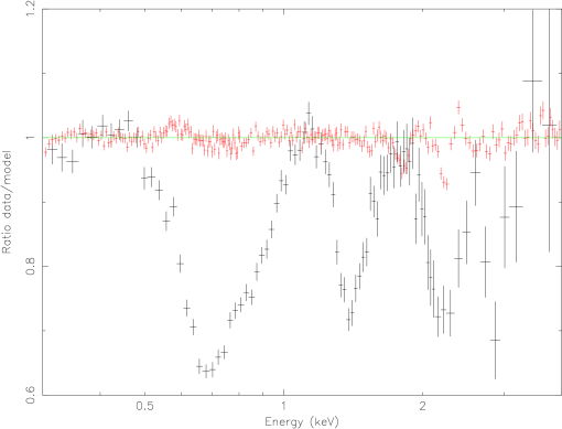
Figure 4: Ratio of the data to the continuum best fit models for 1E 1207.4–5209 (black points) and for the bright quasar 3C 273 (red points). The EPIC/pn observation of 3C 273 (performed on 2001/06/13; pn operated in Small Window mode with the Medium filter) yielded $\sim$62 ksec of good exposure time. PATTERN 0-4 events were extracted from a 43^′′ radius region centered on the source position. Ad-hoc response files were generated. The best fit ($\chi^{2}_{\nu}=1.29$, 1099 d.o.f.) spectral model in the range 0.3-6 keV is a slightly absorbed (N${}_{H}\sim 1.2\times 10^{20}$ cm^-2) double power law (photon indices $\alpha_{ph\leavevmode\nobreak\ 1}\sim 2.79$ and $\alpha_{ph\leavevmode\nobreak\ 2}\sim 1.43$; 0.3-6 keV fluxes $F_{1}\sim 4.47\times 10^{-11}$ erg cm^-2 s^-1 and $F_{2}\sim 8.67\times 10^{-11}$ erg cm^-2 s^-1). Deviations at the $\sim 6-7$% level are seen in the case of the featureless 3C 273 spectrum owing to residual miscalibrations at the Si (1.839 keV) and Au (2.209 keV) edges. These artefacts can be reproduced ($\chi^{2}_{\nu}=1.05$, 1093 d.o.f.) by two gaussian lines in absorption centered at the edge energies, with equivalent width of $\sim 5.5$ eV and $\sim 7.7$ eV for the Si and the Au edge case, respectively. The $\sim$2.1 keV feature seen in the spectrum of 1E 1207.4–5209 (see text and Table 2) is markedly stronger, with a $>$13 times higher equivalent width, and is totally unrelated to the calibration leftovers which are never seen in dim sources.

The large number of photons allows to determine with high accuracy the profiles of the two main features. A simple gaussian is inadequate to reproduce the broad dips, owing to their asymmetric shape. The combination of two gaussian lines in absorption can mimic their profile yielding a statistically good fit ($\chi^{2}_{\nu}\sim 1.0$, 92 d.o.f.). We found that a good fit can be also obtained using an asymmetric line profile having the following analytic form:

$$A(E)=\exp[-a(E-E_{0})^{2}-b(E-E_{0})^{3}-c(E-E_{0})^{4}]$$ (1)

We note that this model does not have a direct physical meaning. Rather, it is used to phenomenologically describe the data, since it allows for an easy evaluation of the central energy of the features and reproduces their shape with a small number of parameters. We therefore adopt this model to fit the two main features at 0.7 and 1.4 keV; the third and the fourth features, owing to the lower statistics, can be well reproduced by simple gaussian lines in absorption.

The results of the pn data analysis are reported in Table  2.

Figure 5: Fit of the phase-integrated data. The model (double blackbody plus line components) is described in the text. From top to bottom, the panels show data from the pn, the MOS1 and the MOS2 cameras. In each panel the data are compared to the model folded through the instrumental response (upper plot); the lower plot shows the residuals in units of sigma.

We turn now to the MOS1 and MOS2 data, encompassing $\sim$73,800 and $\sim$75,600 photons in the 0.3-4 keV range. We found that, also in these cases, the best fitting continuum model ($\chi^{2}_{\nu}$=1.19 for MOS1 - see Fig. 5, middle panel, $\chi^{2}_{\nu}$=1.47 for MOS2 due to the presence of several small wiggles - see Fig. 5, lower panel) is represented by the sum of two blackbody curves. The temperatures and the emitting regions are consistent with the results from the pn camera; the interstellar absorption is found to be somewhat higher in the MOS data (N_H=(1.3$\pm$0.1)$\times 10^{21}$cm^-2). We ascribe this difference to the observed time evolution of the low energy (E$<$0.5 keV) redistribution function of the MOS detectors (Kirsch 2003). This effect is currently under investigation by the calibration team; we therefore consider the pn measurement to be more reliable.

Three absorption features are clearly detected in the MOS spectra (see Fig. 6). The 2.1 keV feature has a chance occurrence probability of order $10^{-3}$ per camera, as estimated by means of an F-test. Owing to the lower statistics, the 2.8 keV feature is only marginally detected by the MOS cameras and was not included in the model. As in the case of the pn, the shape of the two main features was found to be asymmetric and well reproduced by the analytic profile described in Equation 1. The parameters of the 0.7 and 1.4 keV features are consistent with the pn results (see Table  2.); however, due to the smaller number of photons in the MOS data, some of the parameters decribing the second feature are not well constrained. The lower equivalent width of the 2.1 keV feature in the MOS should not be a matter of concern since in this region of the spectrum the model for the MOS and the pn (including a fourth broad feature at 2.8 keV) are different.

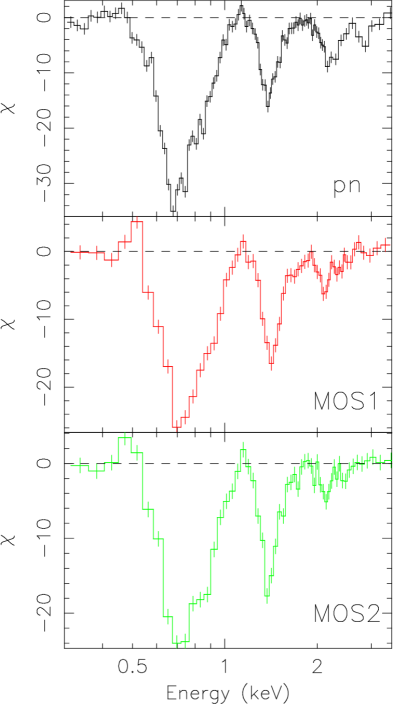
Figure 6: Residuals in units of sigma obtained by comparing the data with the best fit thermal continuum model. The presence of four absorption features at $\sim 0.7$ keV, $\sim 1.4$ keV, $\sim 2.1$ keV and $\sim 2.8$ keV in the pn spectrum is evident. The three main features are also independently detected by the MOS1 and MOS2 cameras.

2.2.2 Phase-resolved spectroscopy

As seen in our first EPIC observation of 1E 1207.4–5209 , the absorption features are phase-dependent (Paper I); in Paper II we showed that the pulse phase variations of the spectrum are stronger in correspondence of the features, while the continuum does not change significantly. This is evident from Fig. 7, where the folded light curves have been plotted in six energy ranges where lines are either dominant (right panels) or nearly absent (left panels). The pulsed fraction is lower ($\sim$4-6%) in the spectral ranges where the features are less important, while is definitely higher ($\sim$10%) in correspondence to the three main features.

Figure 7: Folded light curves of 1E 1207.4–5209 . The energy ranges have been selected in order to put in evidence the impact of the phase variation of the features on the source pulsation. The three panels to the left show that in the spectral regions less affected by the main features the pulsed fraction is of order $\sim$4-6%. The three panels to the right show that the pulsation is much higher ($\sim$10%) in the energy ranges where the three main features are seen.

In order to further investigate such an effect, we extracted phase-resolved spectra. Following Paper II, we selected the phase intervals corresponding to the peak (phase interval 0.40-0.65 with respect to Fig. 3 and  7), the declining part (phase 0.65-0.90), the minimum (phase 0.90-1.15) and the rising part (phase 0.15-0.40) of the folded light curve.

The resulting spectra were fitted allowing both the thermal continuum and the lines to vary. For the sake of simplicity, the fourth feature, owing to its lower significance, was not included in the model.

We give the best fit parameters, describing the phase resolved spectra, in Table  3. Note that systematic uncertainties were not included, as stated in Sect. 2.2. In Fig. 8 we plot the residuals with respect to the continuum to show the phase variations of the features.

The results of the phase resolved spectroscopy can be summarized as follows:

• The two components of the continuum vary slightly (see Table 3) both in temperature and in flux with the pulse phase, accounting for $\sim$3-5% of the source pulsation. A comparison with the values reported in Sect. 2.1 and an inspection of Fig. 7 clearly shows that the phase variation of the features is largely responsible for the observed pulsation of the source.

• the features are strongly dependent on the pulse phase; variations in their width, depth (see Table 3) and shape (see Fig. 8) are evident. The central energy of the 0.7 keV feature (as derived from the phenomenological model) vary at most of 6%, while displacements of the other features are not significant. The 2.8 keV feature is marginally detected only during the minimum and the rise intervals.

• The relative intensity of the first three features varies in phase.

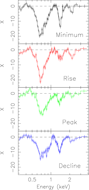
Figure 8: Residuals in units of sigma obtained by comparing the data with the best fit continuum model (line components removed) for the phase-resolved spectra. The variations in width, depth and shape of the absorption features as a function of the pulse phase are evident. Structured residuals are observed in the range 0.4-0.7 keV for the “rise” spectrum and (more significantly) in the range 0.9-1.2 keV in the “decline”, where broad emission features could be present. We did not attempt to model these structures, which are likely artefacts due to an inadequate description of the main absorption features’ profile.

3 Optical data analysis

The field of 1E 1207$-$5209 was observed in Service Mode between April and July 2002 with the 8.2-meter UT-1 Telescope (Antu) of the ESO VLT (Paranal Observatory). Observations were performed with the the FOcal Reducer and Spectrograph 1 (FORS1) instrument, operated as imager in its standard resolution mode, with a pixel size of 0$\aas@@fstack{\prime\prime}$2 and a corresponding field of view of $6\aas@@fstack{\prime}8\times 6\aas@@fstack{\prime}8$, large enough to include many reference stars for a precise CCD astrometry. Images were acquired through the Bessel $V$ and $R$ filters for a total integration time of $\sim$2 and 3 hrs, respectively. The total integration time was split in short exposures of 100 s to avoid saturation of two relatively bright stars (star A and B - Bignami et al. 1992) close to the position of our target and allow for an efficient cosmic ray filtering. Table  1 reports the complete journal of the observations. Exposures were acquired under dark time conditions at airmass $\langle\sec z\rangle\sim 1.5$ and with average seeing of $\sim 0\aas@@fstack{\prime\prime}7$ and $\sim 0\aas@@fstack{\prime\prime}9$ in the $V$ and $R$ bands, respectively. Atmospheric conditions were good, with little wind and humidity always below 10%. All nights were photometric.

Standard reduction steps including debiassing and flatfielding were applied through the ESO FORS1 data reduction pipeline. Flux calibration was performed using images of photometric standards from the Landolt fields (Landolt 1992), yielding extinction and color-corrected zero-points with an overall accuracy of a few hundredths of magnitude. Night-to-night zero-point variations were found to be below 0.04 magnitudes. For each filter, images taken in different nights have been registered and averaged using a 3 $\sigma$ clipping algorithm to reject cosmic ray hits.

In order to register accurately the target position on the FORS1 images, we have recomputed the image astrometry using as a reference the positions of 20 well-suited, (i.e. not extended, not too faint, and not too close to the CCD edges) stars selected from the Guide Star Catalogue II. The overall accuracy of our astrometric solution was of $0\aas@@fstack{\prime\prime}17$ per coordinate.

Fig. 9 shows the inner portion of the combined FORS1 $V$-band image centered on the target position, with the MOS1, MOS2 and ACIS error circles superimposed.

A faint object (marked with the two ticks in Fig. 9) is detected just outside the southern edge of the MOS1 error circle and showed variability along the time span covered by our observations (see caption of Fig. 9). Its position, in any case, falls more than 2^′′ away from the most probable one and we can rule it out as a potential counterpart of 1E 1207.4–5209 .

No candidate counterpart is detected in the Chandra error circle (nor in the intersection of the MOS ones) down to R$\sim$27.1 and V$\sim$27.3, which we assume as upper limits on the optical flux of 1E 1207$-$5209.

Date	Filter	No. of exp.	Exposure(s)	seeing (”)	airmass
2002 April 22	$R$	43	4 300	1.0”	1.33
2002 May 10	$R$	4	400	0.8”	1.034
2002 July 9	$R$	38	3 800	0.58”	1.134
2002 July 9	$V$	26	2 600	0.58”	1.134
2002 July 13	$V$	26	2 600	0.52”	1.054
2002 July 14	$V$	26	2 600	0.96”	1.017
2002 July 15	$R$	26	2 600	0.96”	1.017

Table 1: Summary of the optical observations of the field of 1E 1207$-$5209 performed with the FORS1 instrument at VLT/Antu.

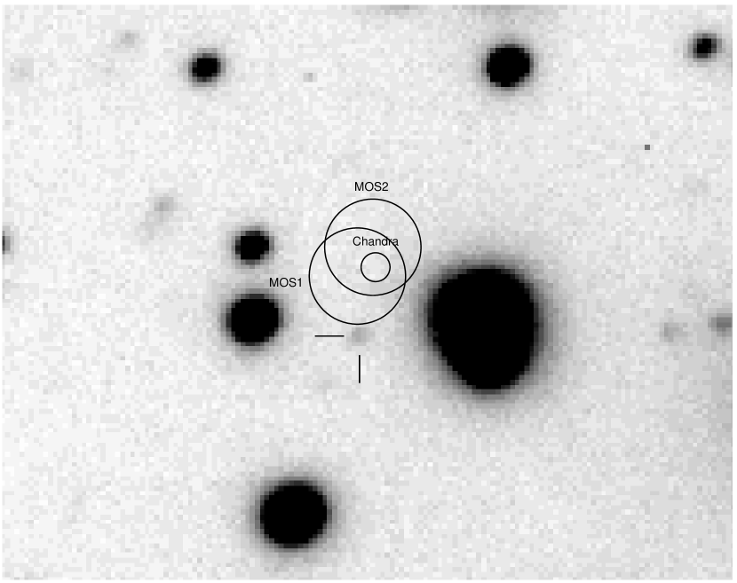
Figure 9: Combined $V$-band FORS1 image of the central region of the 1E 1207$-$5209 field. The circles indicate the expected source positions computed from the Chandra/ACIS (0.6^′′ radius), MOS1 and MOS2 (2^′′ radius) data. The good agreement among the three independent positions gives us confidence on the overall correctness of our analysis. No sources down to R$\sim$27.1 and V$\sim$27.3 are seen inside the error circles. The object labelled with the two small ticks, visible also in the NTT observation of Bignami et al. (1992), falls just outside of the MOS1 error circle. Its time-integrated magnitude in the combined images is $V\sim 25.8$ and $R\sim 24.5$, with uncertainties of $\sim 0.1$ magnitudes. Its profile is consistent with a stellar-like object. Its flux varied of $\sim 0.4$ magnitudes in the $V$-band images (from $V\sim 26.2$ to $V\sim 25.7$), collected during 3 nights, and of $\sim 1.5$ magnitudes in the $R$-band images, collected during 4 nights. It is most probably a background AGN.

4 Discussion

4.1 The thermal continuum emission

The X-ray spectral energy distribution of 1E 1207.4–5209 shows a continuum emission of purely thermal origin which is well reproduced by the sum of two blackbody curves.

Thanks to the unprecedented throughput of the EPIC pn camera, we detected with high statistical significance the variation of the X-ray continuum with the pulse phase. The two blackbody components show a low amplitude ($\leq$5%) modulation in both temperature and flux. This strongly suggests a non-uniform temperature distribution on the neutron star surface. The colder blackbody component (kT$\sim$0.16 keV) is emitted from a quite large fraction of the surface ($R\sim 4.5$ km), while the hotter (kT$\sim$0.3 keV) is possibly coming from a heated polar cap ($R\sim 800$ m). The use of a more physical continuum model (i.e. a magnetized atmosphere model) could yield lower surface temperatures and larger emitting radii, as observed in several cases (e.g. for Vela, Pavlov et al. 2001). The phase shift of $\sim 90^{\circ}$ observed between the peaks of the light curves below and above 0.5 keV requires an energy-dependent asymmetry in the emission pattern.

The optical upper limits fall more than two orders of magnitude above the extrapolation of the best fit X-ray blackbody curves. For a distance of 2 kpc, after dereddening for an absorption $A_{V}\sim$0.6, the upper limit on the optical luminosity $L_{opt}$ is $\sim 3.4\times 10^{28}$ erg s^-1. Using the estimate of the total rotational energy loss obtained from the X-ray timing, $\dot{E}_{rot}$ = (7.4$\pm$1.5)$\times$10³³ erg s^-1, we derive an optical emission efficiency $L_{opt}/\dot{E}_{rot}<4.6\times 10^{-6}$. This value is comparable to the optical emission efficiency of middle-aged neutron stars like PSR B0656+14 and Geminga.

4.2 The absorption features as cyclotron absorption lines

The reanalysis of the long EPIC observation, taking advantage of the recent improvements in the instrument calibration, yielded a more significant detection of the absorption features at 2.1 keV and 2.8 keV. The conclusion of Paper II is therefore strenghtened: the presence of four absorption features, having central energies very close to the ratio 1:2:3:4, coupled with their observed phase variation, is naturally explained by cyclotron absorption from one fundamental and three harmonics.

The absorption features are seen during all phase intervals. The absorbing layer is therefore surrounding most (all) of the X-ray emitting region. The observed $\Delta E/E$ of the features, about 0.1$\div$0.3 depending on the phase interval, implies that the variation of the magnetic field across the line forming region ($\Delta E/E\sim\Delta B/B$) is very small, constraining both the thickness and the latitudinal extent of the absorbing layer. Assuming for simplicity a standard dipole configuration, the radial dependence of the magnetic field yields $\Delta B/B\sim 3\Delta r/r$. The data therefore constrain the thickness $\Delta r$ to (0.3-1)r₁₀ km, depending on the phase interval, where r₁₀ is the distance (in units of 10 km) of the absorbing layer from the neutron star centre. Moreover, considering the dependence of the dipole field on the latitude, B$\sim(1+3\,\cos^{2}\theta)^{\frac{1}{2}}$, the measured line width implies that the absorbing region is limited in latitude to an interval of 15-30 degrees from the equator, or 30-50 degrees from the pole, depending on the phase interval.

4.3 The cyclotron magnetic field and the pulsar slow-down

The cyclotron interpretation of the absorption features allows for a direct measure of the neutron star magnetic field. This can be compared with the magnetic field value estimated from the observed timing parameters, B = (2.6$\pm$0.3)$\times$10¹² G, assuming an uniform slow-down due to magneto-dipole braking.

Assuming that the 0.7 keV feature corresponds to the fundamental cyclotron energy for electrons or for protons, the inferred magnetic field would be of 0.6(1+z)$\times 10^{11}$ G or 1.2(1+z)$\times 10^{14}$ G, respectively; z represents the gravitational redshift where the absorption occurs. Two hypotheses about the absorbing region position can be explored: (i) in the atmosphere, close to the NS surface and (ii) in the magnetosphere, at a few stellar radii.

In the case of electrons, if the cyclotron features are formed close to the surface, the fundamental cyclotron energy of $\sim$0.7 keV yields B$\sim$8$\times 10^{10}$ G , assuming a standard 25% gravitational redshift. This value is $\sim$ 30 times lower than expected from the observed P and $\dot{P}$. A “braking problem” arises: some additional torque should be acting in order to produce the observed spin-down of the neutron star. A disk from the fallback of supernova ejecta could induce such an additional braking if the system is in the propeller regime. Debris disks have been invoked (Chatterjee et al. 2000) to account for the properties of anomalous X-ray pulsars (AXPs, Mereghetti et al. 2002b). The disk models predict an excess in the optical emission (e.g. Perna et al. 2000); indeed, the detection of a few AXPs in the IR band (e.g. Israel et al. 2003 and references therein) recently renewed attention to the disk hypothesis. Although the actual properties of such systems are largely unconstrained, in the case of 1E 1207.4–5209 the optical upper limits would require any hypothetical disk to be underluminous. As a consequence, this scenario appears rather unlikely. Alternatively, the cyclotron absorption could take place in the magnetosphere, as discussed by Sanwal et al. (2002). Sturner & Dermer (1991) and Dermer & Sturner (1994) have suggested that a layer of accreted plasma could form in the magnetosphere of a neutron star, at a height of a few stellar radii, supported by radiation pressure. An alternative possibility is represented by the presence of a “blanket” of $e^{+}$/$e^{-}$ pairs formed in the closed line region of the neutron star magnetosphere at an altitude of $\sim$3 stellar radii (Wang et al. 1998). Although the actual suspended mass, the density, as well as the stability of the suspended absorbing layer are highly uncertain, we note that in this picture the inferred surface magnetic field would be very close to the value expected from the spin parameters.

In the case of proton absorption, the inferred magnetic field would be at least of $1.6\times 10^{14}$ G (absorption occurring at the surface). Such a “magnetar”-like field would not be free from problems when considering the measured $\dot{P}$. The spin-down expected from the standard dipole formula would be much larger than observed, $\sim 6\times 10^{-11}$ s s^-1. A possibility for solving this problem could be the presence of higher multipole components in the magnetic field of the neutron star, as suggested by Sanwal et al. (2002). The surface value could exceed $10^{14}$ G, while the braking would be driven by the dipole component, dominating at large radii.

4.4 A $\dot{P}$ problem ?

The magnetic field inferred from the observed spin-down is hardly conciliable with the independent estimates offered by the cyclotron interpretation of the absorption features. Furthermore, our refined $\dot{P}$ value (see Sect. 2.1) confirms the “age problem” (Pavlov et al. 2002): the characteristic age of 1E 1207.4–5209 , $\tau_{c}$ = (4.7$\pm$1.0)$\times$10⁵ yrs, is more than 50 times higher than the age of the associated supernova remnant ($\tau_{SNR}$ $\sim 7$ kyrs).

To reconcile this discrepancy the possibility of a birth period close to the present one was proposed (Pavlov et al. 2002; Paper I). The same born-slow hypothesis was suggested to solve similar age inconsistencies in few other cases (e.g. PSR J1811-1925 in G11.2-0.3, Kaspi et al. 2001; PSR J0538+2817 in S147, Kramer et al. 2003). Such sources represent a big problem for massive stars core-collapse theory, since it is difficult to explain initial spin periods as large as a few tens of milliseconds (Heger et al. 2003).

Of course, all of the above assumes 1E 1207.4–5209 to be a smoothly slowing down pulsar. If the period evolution of the source is not monotonic, our measurement of the period derivative, based on a set of sparse observations, could be wrong. For example, glitches could dominate the long-term spin-down of the source, which would appear lower than that due to the magnetodipole radiation. The $\dot{P}$ measurement might also be affected by Doppler shift, if the neutron star is in a binary system. In this case, the optical upper limits ($R>27.1$, $V>27.3$), for a distance of 2 kpc and an absorption $A_{V}\sim 0.6$, exclude any main sequence star as a possible companion to 1E 1207.4–5209 , leaving open only the possibility of a degenerate object.

We note that a very recent (June 2003) Chandra observation of 1E 1207.4–5209 did not help to clarify the issue of the period evolution of the source (see Zavlin et al. 2003).

4.5 1E 1207.4–5209 : out of the chorus line ?

An important problem still lacking a solution concerns the uniqueness of the phenomenology of 1E 1207.4–5209 in the isolated neutron stars panorama. High quality X-ray observations have been performed on several isolated neutron stars of various kind. The detection of absorption features has been claimed only in the Soft Gamma Repeater 1806-20 (Ibrahim et al. 2002,2003), in the Anomalous X-ray Pulsar 1RXS 170849–400910 (Rea et al. 2003) and in the isolated neutron stars RBS 1223 (Haberl et al. 2003) and RX J1605.3+3249 (van Kerkwijk 2003). None of these cases is comparable to the phenomenology of 1E 1207.4–5209 .

A possible explanation invokes selection effects. 1E 1207.4–5209 could be an “unconventional”, low magnetic field neutron star ($<10^{11}$ G as in the electron, near-surface cyclotron scenario). In sources with more typical magnetic fields of order $10^{12}$ G the cyclotron energy would lie in the range of the tens of keV, where the surface thermal emission is very low and where sensitive X-ray observations have not yet been obtained. If the magnetic field of 1E 1207.4–5209 , on the contrary, is closer to the typical value of $10^{12}$ G (as in the magnetospheric cyclotron scenario), the absence of cyclotron features in other sources could be explained by a limited lifetime for the absorbing layer.

An answer to the “uniqueness problem” could come only through a better understanding of the overall properties of the Central Compact Obiects in supernova remnants, the fraternity of 1E 1207.4–5209 . These sources are supposed to be the youngest members of the radio-quiet neutron stars family (including also Anomalous X-ray Pulsars, Soft Gamma Repeaters and Dim Thermal Neutron Stars), but their physics remain elusive. We do not understand the lack of radio emission, the lack of X-ray pulsations (1E 1207.4–5209 being unique, at the moment, also in this aspect of the phenomenology). The fallback of supernova ejecta is possibly playing an important role, driving their multiwavelength emission, their spin-down and their evolution, as suggested by Alpar (2001). Deeper observations of these sources could shed light to the overall scenario. Only in this perspective we will have an answer to the question whether 1E 1207.4–5209 is indeed an unique object, or is simply in a standard (transient) phase of the evolution of a young neutron star.

Table 2: Results of phase-integrated spectroscopy

	pn	MOS1	MOS2
NH (1021 cm-2)	1.0$\pm 0.1$	1.4$\pm 0.1$	1.3$\pm 0.1$
kTBB1 (keV)	0.164$\pm$0.001	0.165$\pm$0.002	0.168$\pm$0.002
R${}_{BB1}^{(a)}$ (km)	4.5$\pm$0.1	4.6$\pm$0.1	4.6$\pm$0.1
kTBB2 (keV)	0.319$\pm$0.002	0.322$\pm$0.002	0.320$\pm$0.002
R${}_{BB2}^{(a)}$ (km)	0.83$\pm$0.02	0.83$\pm$0.03	0.83$\pm$0.03
E1 (keV)	0.68$\pm$0.01	0.69$\pm 0.01$	0.69$\pm 0.01$
a1	77${}^{+2}_{-3}$	80$\pm$3	82$\pm$3
b1	-368${}^{+7}_{-22}$	-419$\pm$15	-412$\pm$15
c1	616${}^{+26}_{-44}$	749$\pm$40	684$\pm$40
EW1 (eV)	99${}^{+4}_{-7}$	105${}^{+6}_{-7}$	104${}^{+6}_{-7}$
FWHM1 (keV)	0.24$\pm 0.01$	0.24$\pm 0.02$	0.24$\pm 0.02$
E2 (keV)	1.36$\pm$0.01	1.39$\pm 0.02$	1.37$\pm 0.02$
a2	96${}^{+8}_{-32}$	89${}^{+33}_{-11}$	96${}^{+27}_{-8}$
b2	-370${}^{+50}_{-20}$	-360${}^{+250}_{-30}$	-220${}^{+270}_{-35}$
c2	488${}^{+145}_{-55}$	220${}^{+1000}_{-55}$	500${}^{+1000}_{-80}$
EW2 (eV)	66$\pm 6$	64$\pm 7$	67$\pm 7$
FWHM2 (keV)	0.18$\pm 0.02$	0.19$\pm 0.03$	0.20$\pm 0.03$
E3 (keV)	2.14$\pm$0.03	2.12$\pm$0.07	2.12$\pm$0.08
$\sigma_{3}$ (keV)	0.17$\pm$0.03	0.13${}^{+0.10}_{-0.04}$	0.10${}^{+0.10}_{-0.04}$
$EW_{3}$ (eV)	94$\pm 15$	48$\pm 20$	45$\pm 20$
E4 (keV)	2.83$\pm$0.05	–	–
$\sigma_{4}$ (keV)	0.11${}^{+0.10}_{-0.04}$	–	–
$EW_{4}$ (eV)	81${}^{+20}_{-30}$	–	–
F${}_{0.3-4keV}^{(b)}$ (erg cm-2 s-1)	2.24$\times 10^{-12}$	2.10$\times 10^{-12}$	2.17$\times 10^{-12}$
L${}_{X}^{(c)}$ (erg s-1)	2.1$\times 10^{33}$	2.2$\times 10^{33}$	2.2$\times 10^{33}$
$\chi^{2}$/dof	1.15	1.19	1.47
dof	94	154	151

^a Radius at infinity for an assumed distance of 2 kpc.

^b Observed flux.

^c Bolometric luminosity for d=2 kpc.

All the errors are at the 90% c.l. for a single interesting parameter

Table 3: Results of phase resolved spectroscopy

	Minimum	Rise	Peak	Decline
NH (1021 cm-2) fixed	1.0	1.0	1.0	1.0
kTBB1 (keV)	0.157$\pm$0.001	0.156$\pm$0.001	0.171$\pm$0.002	0.164$\pm$0.002
R${}_{BB1}^{(a)}$ (km)	4.67$\pm$0.03	4.85$\pm$0.06	4.01$\pm$0.03	4.20$\pm$0.04
kTBB2 (keV)	0.297$\pm$0.002	0.302$\pm$0.002	0.293$\pm$0.002	0.290$\pm$0.002
R${}_{BB2}^{(a)}$ (km)	1.00$\pm$0.01	0.98$\pm$0.03	1.04$\pm$0.01	1.12$\pm$0.03
E1 (keV)	0.664$\pm$0.005	0.679$\pm$0.005	0.703$\pm$0.006	0.668$\pm$0.012
a1	94.4$\pm$1.5	98.2${}^{+3.4}_{-2.6}$	78.7${}^{+1.9}_{-1.8}$	70.1${}^{+1.5}_{-12.1}$
b1	-499${}^{+6}_{-5}$	-464${}^{+15}_{-9}$	-320${}^{+7}_{-6}$	- 403${}^{+11}_{-9}$
c1	848${}^{+21}_{-20}$	762${}^{+51}_{-34}$	424${}^{+23}_{-17}$	724${}^{+21}_{-37}$
EW1 (eV)	114${}^{+4}_{-5}$	103${}^{+5}_{-6}$	92${}^{+5}_{-5}$	93${}^{+5}_{-3}$
FWHM1 (keV)	0.22$\pm$0.01	0.19$\pm$0.01	0.21$\pm$0.01	0.32$\pm$0.02
r${}_{1}^{(b)}$	0.46$\pm$0.02	0.43$\pm$0.02	0.29$\pm$0.02	0.30$\pm$0.02
E2 (keV)	1.37$\pm$0.01	1.38$\pm$0.02	1.33$\pm$0.01	1.35$\pm$0.01
a2	147$\pm$11	34.5$\pm$0.5	171${}^{+16}_{-5}$	63.3${}^{+0.8}_{-0.5}$
b2	-690${}^{+62}_{-38}$	-7.33${}^{+0.09}_{-0.01}$	-981${}^{+73}_{-19}$	-121${}^{+1}_{-2}$
c2	1087${}^{+333}_{-137}$	0.213${}^{+0.010}_{-0.002}$	1629${}^{+216}_{-68}$	60.3${}^{+1.0}_{-0.8}$
EW2 (eV)	82$\pm$6	66$\pm$8	54$\pm$6	93$\pm$7
FWHM2 (keV)	0.14$\pm$0.02	0.35$\pm$0.04	0.14$\pm$0.02	0.21$\pm$0.02
r${}_{2}^{(b)}$	0.41$\pm$0.02	0.19$\pm$0.03	0.19$\pm$0.03	0.32$\pm$0.02
E3 (keV)	2.16$\pm$0.05	2.15$\pm$0.06	2.12$\pm$0.04	2.08$\pm$0.06
$\sigma_{3}$ (keV)	0.09$\pm$0.04	0.14$\pm$0.05	0.08$\pm$0.06	0.08$\pm$0.06
EW3 (eV)	64${}^{+19}_{-19}$	102${}^{+35}_{-40}$	28${}^{+13}_{-13}$	17${}^{+11}_{-11}$
r${}_{3}^{(b)}$	0.25$\pm$0.06	0.29$\pm$0.06	0.13$\pm$0.06	0.15$\pm$0.06
$\chi^{2}$/dof	1.09	1.20	1.35	1.01
dof	79	79	78	78

^a Radius at infinity for an assumed distance of 2 kpc.

^b Relative line depth = 1. – F (E_line) / F_C (E_line), where F is the total flux and F_C is the flux of the continuum only

All the errors are at the 90% confidence level for a single interesting parameter

References

- (1) Alpar, M.A., 2001, ApJ, 554, 1245
- (2) Becker, W. & Aschenbach, B., 2002, Proceedings of the 270. WE-Heraeus Seminar on Neutron Stars, Pulsars, and Supernova Remnants, W. Becker, H. Lesch, and J. Trümper eds., p.64
- (3) Bignami, G.F., Caraveo, P.A. & Mereghetti, S. 1992, ApJ, 389, L67.
- (4) Bignami, G.F., Caraveo, P.A., De Luca, A. & Mereghetti, S. 2003, Nature, 423, 725 (Paper II)
- (5) Chatterjee, P., Hernquist, L. & Narayan, R., 2000, ApJ, 534, 373
- (6) Dermer, C.D. & Sturner, S.J., 1991, ApJ, 382, L23
-
(7)
Ghizzardi, S., 2001, XMM-SOC-CAL-TN-0022, available from
http://xmm.vilspa.esa.es/external/xmm_sw_cal/calib/documentation.shtml#EPIC - (8) Giacani E.B., Dubner, G.M., Green, A.J., et al. 2000, AJ, 119, 281.
- (9) Haberl, F., Schwope, A.D., Hambaryan, V., et al. 2003, A&A, 403, L19
- (10) Hailey, C.J. & Mori, K., 2002, ApJ, 578, L133
- (11) Helfand, D.J. & Becker, R.H., 1984, Nature, 307, 215
- (12) Heger, A., Woosley, S.E., Langer, N. & Spruit, H.C., to appear in “Stellar Rotation”, Proc. IAU 215, astro-ph/0301374
- (13) Ibrahim, A.I., Safi-Harb, S., Swank, J.H., et al. 2002, ApJ, 574, L51
- (14) Ibrahim, A.I., Swank, J.H. & Parke, W. 2003, ApJ, 584, L17
- (15) Israel, G.L., Covino, S., Perna, R., et al. 2003, ApJ, 589, L93
- (16) Kellett, B.J., Branduardi-Raymont, G., Culhane, J.L., et al. 1987, MNRAS, 225, 199
- (17) Kaspi, V.M., Roberts, M.E., Vasisht, G., et al. 2001, ApJ, 560, 371
- (18) Kirsch, M. (on behalf of the EPIC collaboration), EPIC Calibration issues in progress, Document XMM-SOC-CAL-TN-0018-2-1 (EPIC Status of Calibration and Data Analysis), XMM Science Operation Centre, Villafranca del Castillo, 2003, available from http://xmm.vilspa.esa.es/external/xmm_sw_cal/calib/index.shtml
- (19) Kramer, M., Lyne, A.G., Hobbes, G., et al. 2003, ApJ, 593, L31
- (20) Leahy D.A. 1987, A&A, 180, 275.
- (21) Landolt, A.U., 1992, AJ, 104, 340
- (22) Mereghetti S., Bignami G.F. & Caraveo P.A. 1996, ApJ, 464, 842.
- (23) Mereghetti, S., De Luca, A., Caraveo, P.A. et al. 2002a, ApJ, 581, 1280 (Paper I)
- (24) Mereghetti, S., Chiarlone, L., Israel, G.L. & Stella, L., 2002b, Proceedings of the 270. WE-Heraeus Seminar on Neutron Stars, Pulsars, and Supernova Remnants, W. Becker, H. Lesch, and J. Trümper eds., p.29
- (25) Pavlov, G.G., Zavlin, V.E., Sanwal, D., et al. 2001, ApJ, 552, L129.
- (26) Pavlov, G.G., Zavlin, V.E., Sanwal, D. & Trümper, J. 2002, ApJ, 569, L95.
- (27) Perna, R., Hernquist, L. & Narayan, R., 2000, ApJ, 541, 344
- (28) Rea, N., Israel, G., Stella, G.L., et al. 2003, ApJ, 586, L65
- (29) Roger, R.S., Milne, D.K., Kesteven, M.J., et al. 1988, ApJ, 322, 940.
- (30) Sanwal D., Pavlov, G.G., Zavlin, V.E & Teter, M.A. 2002, ApJ, 574, L61
- (31) Strüder L., Briel, U., Dennerl, K., et al. 2001, A&A, 365, L18
- (32) Sturner, S.J. & Dermer, C.D., 1994, A&A, 284, 161
- (33) Turner, M.J.L., Abbey, A., Arnaud, M., et al. 2001, A&A ,365, L27
- (34) van Kerkwijk, M. H., to appear in “Young Neutron Stars and Their Environments”, Proc. IAU 218, astro-ph/0310389
- (35) Vasisht, G., Kulkarni S.R., Anderson, S.B., Hamilton, T.T. & Kawai, N. 1997, ApJ, 476, L43.
- (36) Wang, F.Y.-H., Ruderman, M., Halpern, J.P. & Zhu, T., 1998, ApJ, 498, 373
- (37) Xu, R.X., Wang, H.G. & Quiao, G.J. 2003, Chin.Phys.Lett. 20, 314, astro-ph/0207079
- (38) Zavlin V.E., Pavlov G.G., Sanwal D. & Trümper J. 2000, ApJ, 540, L25.
- (39) Zavlin V.E., Pavlov G.G., Sanwal D., 2003, submitted to ApJ, astro-ph/0312096