Visibility of Old Supernova Remnants in Hi 21-cm Emission Line

Abstract

We estimate the number of old, radiative supernova remnants (SNRs) detectable in Hi 21-cm emission line in the Galaxy. We assume that old SNRs consist of expanding Hi shells and that they are visible if the line-of-sight velocities are sufficiently outside the velocity range of the Galactic background Hi emission. This criterion of visibility makes it possible to calculate the background contamination and to make a comparison with observation. The Galactic disk in our model is filled with atomic gas of moderate ($\sim 0.1$ cm^-3) density representing the warm neutral interstellar medium. We assume that only Type Ia supernovae produce isolated SNRs with expanding Hi shells, or “Hi SNRs”. According to our result, the contamination due to the Galactic background Hi emission limits the number of visible SNRs to $\simeq 270$, or $\simeq 9$% of the total Hi SNRs. They are concentrated along the loci of tangential points. The telescope sensitivity further limits the number. We compare the result with observations to find that the observed number ($\leq 25$) of Hi SNRs is much less than the expected. A plausible explanation is that previous observational studies, which were made toward the SNRs identified mostly in radio continuum, missed most of the Hi SNRs because they are too faint to be visible in radio continuum. We propose that the faint, extended Hi 21-cm emission line wings protruding from the Galactic background Hi emission in large-scale $(\ell,v)$ diagrams could be possible candidates for Hi SNRs, although our preliminary result shows that their number is considerably less than the expected in the inner Galaxy. We conclude that a possible explanation for the small number of Hi SNRs in the inner Galaxy is that the interstellar space there is largely filled with a very tenuous gas as in the three-phase ISM model, not with the warm neutral medium of moderate density.

1 Introduction

A general picture of old SNRs is a hot bubble surrounded by a dense, atomic shell. The shell is preceded by SNR shock, which is radiative. A shock is referred to as “radiative” if the cooling time of the shock-heated material is shorter than the age of the shock. For the SNR shock propagating in a uniform, homogeneous medium of hydrogen density $\sim 1$ cm^-3, it becomes radiative when the SNR is $\sim 3.6\times 10^{4}$ yrs old, or when the shock velocity drops to $\sim 180$ km s^-1 (see Section 2.3). The shell decelerates as it sweeps out more material, and, eventually, when the SNR is $\sim 10^{6}$ yrs old, the velocity of the shell drops to an order of the ambient sound speed ($\sim 10$ km s^-1) and the SNR merges into the general interstellar medium (ISM). We may call old SNRs with fast-expanding Hi shells “Hi SNRs” because they are observable in Hi 21-cm emission line.

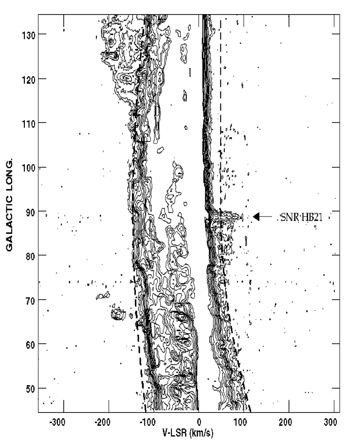
Figure 1: ($\ell,v$) diagram of Hi 21-cm emission at $b=5.^{\circ}0$. Notice the excess emission at the position of the SNR HB 21 ($\ell=89^{\circ}$) between 40 and 100 km s^-1. The dashed lines represent the boundaries of the Galactic background emission used in our model (see Section 2.4). The map has been made from the Leiden-Dwingeloo Hi survey data (Hartmann & Burton, 1997), and the contour levels start at 0.1 K and end at 10 K.

A systematic Hi 21-cm line observation of SNRs to detect the expanding shells have been made by Koo & Heiles (1991; hereafter KH91). It is difficult to detect expanding Hi shells, because most known SNRs are located in the Galactic plane where the Galactic background Hi emission causes severe contamination. There had been papers reporting the detection of Hi shells with expansion velocities smaller than $\sim$20 km s^-1, but the association was rather ambiguous (Assousa & Erkes, 1973; Knapp & Kerr, 1974; Colomb & Dubner, 1980, 1982). If the expansion velocity of the shell is very large, larger than the maximum velocity permitted by the Galactic rotation, however, then it could be easily discernable from the background emission. Fig.  1 shows such an example, where we can clearly see an extended high-velocity (HV) excess emission localized at the position of the SNR HB 21. The positional coincidence and the forbidden velocity strongly suggest that the excess emission is emitted from the gas accelerated by the SNR shock. KH91 carried out a sensitive survey of Hi 21 cm emission lines toward 103 northern Galactic SNRs and detected such HV gas toward 15 SNRs, including 3–4 SNRs known prior to the survey (DeNoyer 1978; Giovanelli & Haynes 1979; Landecker, Roger, & Higgs 1980; Braun & Strom 1986; Koo et al. 1990). Koo, Kang, & McClure-Griffiths (2003) searched for similar Hi features toward 97 southern SNRs using the Southern Galactic Plane Survey data (McClure-Griffiths 2001) and identified another 10 SNRs. These $25(=15+10$) SNRs are candidates for Hi SNRs because the surveys were made using single-dish radio telescopes with a large ($36^{\prime}$ or 16^′) beam size and high-resolution observational studies are necessary for confirming the nature of the HV emission. Such high-resolution studies have been done for some of the SNRs and confirmed the shell-like structure of the HV Hi features, e.g., CTB 80 (Koo et al., 1990), W44 (Koo & Heiles, 1995), W51C (Koo & Moon, 1997), and IC 443 (Giovanelli & Haynes, 1979; Braun & Strom, 1986). But molecular lines studies showed that the latter three SNRs exhibit evidences for the interaction with molecular clouds, e.g., broad molecular lines, high-ratio of high- to low-transition CO lines, 1720-MHz maser line of the OH molecule, etc. (see Koo 2003 and references therein). The HV Hi gas in these SNRs is possibly formed by a radiative shock propagating through molecular clouds, not by the shock propagating through the general diffuse ISM. In summary, including the ones interacting with molecular clouds, there are 25 Hi SNR candidates which appear to have shock-accelerated Hi gas at velocities forbidden by the Galactic rotation.

How does this compare to the expected number of Hi SNRs in the Galaxy? If we naively multiply the total supernova rate ($\sim 0.02$ yr^-1) in the Galaxy to the lifetime ($\sim 1\times 10^{6}$ yr) of SNRs, we get $\sim 2\times 10^{4}$. The majority of supernovae (SNe), however, are core-collapse SNe with massive progenitors. Massive stars are born in associations, and most of these SNe dissipate their energy in producing superbubbles instead of isolated SNRs. Also, a significant fraction of SNe occur in the Galactic halo where they merge into the ambient ISM before cooling becomes important. And, if the structure of the ISM is close to the three-phase model of the McKee & Ostriker (1977) so that most of the interstellar space is filled with hot tenuous ($3.5\times 10^{-3}$ cm^-3) medium, the SNRs may overlap with other SNRs before dense shell formation. Meanwhile, the majority of Hi SNRs may not be visible because of the contamination due to the Galactic background emission and the limited sensitivity. The effect of the background contamination is difficult to calculate in general, which hampers the estimation of the number of visible SNRs. But, for the Hi SNRs, if we limit to the ones with large expansion velocities as in Fig. 1, it is straightforward to calculate the effect because the boundary of the background emission in Fig. 1 is mainly determined by the Galactic rotation. Therefore, the statistics of such Hi SNRs can be related to the Galactic distribution of SNe, their environments, and the evolution of their remnants.

In this paper, we develop a model to estimate the visibility of Hi SNRs in the Galaxy. The outline of the paper is as follows: in Section 2 we describe our model and formulation. We model the Galactic disk as an axi-symmetric, uniform, homogeneous disk with a central hole. We estimate the frequency and distribution of SNe in the disk using recent observational results on extragalactic SNe and old disk stars. We summarize the dynamical evolution of old SNRs in homogeneous, uniform medium and devise the detection probability. Section 3 presents the results, where we show the expected distribution of Hi SNRs in the Galactic plane and their statistics. We explore how the background contamination and the telescope sensitivity limit the visible number of Hi SNRs. In Section 4, we discuss the effect of embedded clouds and compare the result with observations.

2 DESCRIPTION OF MODEL

2.1 Galactic Hi Disk and Hi SNRs

What would be the nature of the ISM that a typical isolated SNR experiences? This is perhaps the very essential question in deriving the number of Hi SNRs because the formation and evolution of dense radiative shells depend on the physical properties of the ambient ISM. A general picture of the ISM is dense clouds immersed in a diffuse intercloud medium, perhaps except regions surrounding OB stars where the clouds might have vanished through photoevaporation and rocket effect due to strong UV radiation (e.g., McKee, Van Buren, & Lazareff 1984). The birthplaces for the isolated SNe are presumably far from OB stars, so as to be close to the general ISM. Then, although the embedded clouds may modify the internal structure through evaporation, it is the intercloud medium that primarily controls the dynamical evolution of SNRs (e.g., Cowie, McKee, & Ostriker 1981), and the question is what the physical conditions of the intercloud medium are. There have been substantial studies on this subject, and it is generally considered that the major component of the intercloud medium is either the warm neutral medium (WNM) with a typical density of $\sim 0.1$ cm^-3 as in the two-phase model of Field, Goldsmith, & Habing (1969) or the hot ionized medium (HIM) of $3.5\times 10^{-3}$ cm^-3 as in the three-phase model of McKee & Ostriker (1977) (see McKee 1995 for a review). Relative filling factors of the two phases, however, are poorly known even in the solar neighborhood. If it is the HIM, then most of the SNRs might dissipate their energy without forming a radiative shell, and there will be only a few Hi SNRs. In the following, we calculate the number of Hi SNRs assuming that the intercloud medium is composed with the WNM only, and, by comparing the result with observations, we will infer the structure of the ISM.

We assume that the Hi gas in the Galaxy is confined to an axi-symmetric, center-emptied disk with an inner edge at 3.5 kpc and outer edge at 15 kpc. The total Hi column density perpendicular to the Galactic plane is approximately constant between 3.5 kpc and 20 kpc, but has a central hole. The inner edge represents the boundary where the Hi surface density drops rapidly (Kulkarni & Heiles, 1987). We take the outer edge of the disk at 15 kpc (instead of 20 kpc) considering that the distribution of isolated SNe are possibly truncated at $\lower 2.15277pt\hbox{$\;\buildrel<\over{\sim}\;$}15$ kpc (see Section 2.2). Even if there is no truncation, the small disk size should not notably affect the result because, as we discuss in Section 2.2, the isolated SNe are considered to be centrally concentrated with a short ($\sim 3$ kpc) exponential radial scale length. We assume that the thickness of the disk is constant and the density distribution is uniform. The real Galactic disk is warped and flares outside the solar circle (Kulkarni, Blitz, & Heiles 1982; Lockman 1984). But this complexity should have little effect on the result because, firstly, most ($\sim 80$%) SNe occur within the solar circle and, secondly, the stellar disk and, therefore the SNe disk, warps and flares too (López-Corredoira et al., 2002). Our formulation is essentially two-dimensional and the primary purpose of considering the thickness of the disk is to estimate the fraction of SNe that explodes in the very tenuous halo, which may not evolve to Hi SNRs (Section 2.2). According to KH91, all the Hi SNR candidates in the inner Galaxy is within $z<200$ pc, while, in the outer Galaxy, the one (CTA 1) located at the farthest from the midplane is at $(r,z)=(10~{}{\rm kpc},370~{}{\rm pc})$ where $r$ is the Galactocentric radius and $z$ is the height above the midplane. The latter corresponds to $314$ pc at $r=r_{\odot}\equiv 8.5$ kpc if we consider that the thickness of the disk flares almost linearly outside the solar circle. Considering this, we adopt the half-thickness of our disk to be 320 pc, i.e., SNe occurring outside this disk are assumed not to form an Hi shell. This is greater than the half-width at half-maximum (265 pc) of the thick Gaussian component and less than the scale height (403 pc) of the exponential component of the Hi disk (Dickey & Lockman, 1990). The total intercloud Hi column density perpendicular to the Galactic plane in the solar neighborhood is $\sim 90$ cm^-3 pc (Heiles, 1987), and we require our model disk to have the same vertical column density. Therefore, the density of our disk $n_{0}=0.14~{}{\rm cm}^{-3}$.

For such axi-symmetric, two-dimensional disk, the number of observable Hi SNRs can be written as

$$N=(\Sigma_{\rm SN}f_{\rm HI})\tau f_{\rm obs},$$ (1)

where $\Sigma_{\rm SN}$ is the total isolated SN rate in the Galaxy, $f_{\rm HI}$ is the fraction of isolated SNe that produces Hi SNRs (i.e., the fraction within the center-emptied model gaseous disk), $\tau$ is the lifetime of Hi SNRs, and $f_{\rm obs}$ the fraction of Hi SNRs that are detectable:

$$f_{\rm obs}\equiv{1\over\Sigma_{\rm SN}f_{\rm HI}\tau}\int\,\sigma_{\rm SN}(r)\int\,p(x,y,t)dtdA$$ (2)

where $\sigma_{\rm SN}(r)$ is the surface density distribution of SNe, i.e., the SN rate per unit area as a function of Galactocentric radius $r$, and $p(x,y,t)$ is the probability that a Hi SNR of age $t$ is detectable considering the background contamination and the telescope sensitivity. $(x,y)$ represents a coordinate grid centered at the Galactic center and the integration range over $(x,y)$ is from $r=3.5$ kpc to 15 kpc. If the detection probability $p(x,y,t)$ is independent of $(x,y)$ and is equal to 1 during $\tau$, then $f_{\rm obs}=1$ and $N=\Sigma_{\rm SN}f_{\rm HI}\tau$. In the following sections, we estimate the individual items in equations (1) and (2).

2.2 Frequency and Distribution of SNe

For our purpose, SNe are divided into two types: Supernovae of type Ia (SNe Ia) which have old disk stars as their progenitors and the “core-collapse” SNe (e.g., type Ib/c and type II SNe; hereafter SNe II) which have massive progenitors. SNe II may be further divided into two groups; ones exploding in associations and the other exploding isolated. Most of the former SNe are expected to explode within a superbubble where the density is very low and pressure is very high. Such SNRs might dissipate their energy before radiative cooling becomes important, and we consider that they do not evolve to Hi SNRs. The latter group is consisted of “runaway” OB stars which are ejected from their parent association and also possibly the OB stars formed isolated. Gies & Bolton (1986) derived that 10–25% of O stars are runaways while only about 2% of early B stars, which contribute most of the SNe, are runaways. This led McKee (1995) to conclude that there is no need to assume a separate population of isolated OB stars. On the other hand, Ferriére (1995) analyzed the catalog of OB stars compiled by Gies (1987) and Humphreys & McElroy (1984), and concluded that 40% of SNe II occurs isolated (see also McKee 1990). Among the historical SNe II, at least Crab is not associated with a group of OB stars and its progenitor could have been a runaway (Mdzinarishvilli & Dzigvashvilli, 2001). We assume that all SNe II explode in groups and that only SNe Ia produce isolated SNRs that can evolve to Hi SNRs. The basic idea is to choose parameters to minimize the number of Hi SNRs when they are uncertain, so that the derived number is to be a lower limit. If the population of isolated OB stars is indeed significant, then the expected number of Hi SNRs will be larger than the calculated below.

The Galactic SN Ia rate is inferred from the extragalactic SN rates, which are usually expressed in SNu or SN (100 yr)^-1 ($10^{10}L_{B}/L_{\odot})^{-1}$ where $L_{B}$ is the blue luminosity of the galaxy (e.g., van den Bergh & McClure 1994; Cappellaro, Evans, & Turatto 1999). Our Galaxy is considered to be a spiral of Hubble type Sb or Sbc with $L_{B}=(2.3\pm 0.6)\times 10^{10}$ $L_{\odot}$ (van den Bergh, 1988), and we take the arithmetic mean of the average rates of S0a-Sb and Sbc-Sd galaxies in Cappellaro et al. (1999) to obtain the total SN Ia rate of $0.45\times 10^{-2}$ yr^-1. (For comparison, the total SN II rate is $1.8\times 10^{-2}$ yr^-1.) It is noted that this SN Ia rate is higher than the one (0.3–0.4$\times 10^{-2}$) derived from the nova rate (van den Bergh & Tammann, 1991), but consistent with the estimate (0.3–0.6$\times 10^{-2}$) of van den Bergh & McClure (1994).

SNe are centrally concentrated and vertically stratified, presumably following the distribution of their progenitors. The progenitors of SN Ia are mostly old disk stars. Bulge stars could contribute as much as $15$% to the total SN Ia rate if the SN rate scales with the mass ratio of the bulge ($\sim 10^{10}$ $M_{\odot}$) to the disk ($\sim 7\times 10^{10}$ $M_{\odot}$) (Dawson, & Johnson, 1994). But the rate of SN Ia within 1 kpc of the center of spiral galaxies has been found to be significantly lower than outside this region (Wang, Höflich, & Wheeler 1997; Hatano, Branch, & Deaton 1998), which suggests that the SN Ia occurs in the bulge not as frequently as expected. The space density of old disk stars perpendicular to the Galactic plane can be accurately represented by the sum of two exponentials, one with a characteristic scale height of $\sim 300$ pc and the other which has a scale height of $\sim 1$ kpc (e.g., Binney & Merrifield, 1998). The latter “thick disk” stars appear older ($\lower 2.15277pt\hbox{$\;\buildrel>\over{\sim}\;$}10^{10}$ yr) and more metal poor ([Fe/H]$\lower 2.15277pt\hbox{$\;\buildrel<\over{\sim}\;$}-0.4$) than the former “thin” disk (Binney & Merrifield, 1998). The total mass of the thick disk stars is $\lower 2.15277pt\hbox{$\;\buildrel<\over{\sim}\;$}10\%$ of the thin disk stars (Trimble 2000). Therefore, if the SN Ia rates of thin and thick disks are proportional to their masses, the thick disk could contribute at most $\lower 2.15277pt\hbox{$\;\buildrel<\over{\sim}\;$}10$% of the thin disk to the total SN Ia rate. We neglect the small uncertain contributions from the bulge and thick disk, and assume that the old stellar disk representing the SN Ia progenitors has a vertical exponential distribution with a scale height of 300 pc at $r=r_{\odot}$. This implies that, in the solar neighborhood, 34% of SNe Ia explodes outside our $\pm 320$ pc-thick gaseous disk. We further assume that this fraction remains constant over the full disk, e.g., we assume that the fraction of SNe Ia exploding in the ‘Hi halo’ and not evolving to Hi SNRs $f_{\rm halo}=0.34$. This is not unreasonable because the old stellar disk warps and flares as the gaseous disk does (Freudenreich, 1998; López-Corredoira et al., 2002). But the flaring of the stellar disk may start well inside the solar circle (López-Corredoira et al., 2002), in which case the assumption of the constant fraction underestimates the SN Ia rate in the inner Galaxy.

The radial surface distribution of old stellar disk is usually described by a single exponential profile, but the radial scale lengths quoted in published papers span an enormous range: 1.8 to 6 kpc (Kent, Dame, & Fazio 1991 and references therein). Recent near-infrared studies based on the the COBE/DIRBE data or the Two Micron All Sky Survey data appear to yield a shorter scale length (2.1–2.8 kpc) consistently (Freudenreich 1998; Ojha 2001; Drimmel & Spergel 2001 and references therein). On the other hand, studies on extragalactic SNe show that, although the number of SN Ia is small (54) to constrain the slope very well, the distribution could be represented by a single radial scale length of $R_{25}/5.5$ where $R_{25}$ is the semimajor axes of isophote having 25.0 mag arcsec^-2 in blue (van den Bergh, 1997). The Andromeda galaxy (M31), for example, has $R_{25}=20$ kpc (Trimble 2000), so that the radial scale length of SN Ia would be $3.6$ kpc. We adopt 3.0 kpc as the radial scale length of the SN Ia surface density distribution in the Galaxy, and assume that the distribution extends all the way to the Galactic center. The stellar disk may have a central hole where a stellar bar is located (Freudenreich, 1998). But, since the surface density profile averaged over the azimuth remains approximately exponential to the center (Freudenreich, 1998), the assumption of an axisymmetric exponential distribution is plausible. Hence, after normalization, the SN rate per unit area in our model disk is given by

$$\sigma_{\rm SN}(r)=\sigma_{0}\exp(-r/3.0~{}{\rm kpc})$$ (3)

where $\sigma_{0}=5.5\times 10^{-5}$ kpc^-2 yr^-1. With the above distribution, the fraction exploding inside the central hole $f_{\rm hole}=0.34$. Therefore, the fraction of isolated SNe that explodes within our model gaseous disk $f_{\rm HI}=(1-f_{\rm halo})(1-f_{\rm hole})=0.44$. The frequency of Hi SNRs in our model Hi disk, therefore, is $\Sigma_{\rm SN}f_{\rm HI}=0.20\times 10^{-2}$ yr^-1, or one per 500 yrs.

2.3 Dynamical Evolution of Hi SNRs

In our model, SNRs evolve in a homogeneous, uniform medium and we are interested in their late-stage evolution. (The effect of embedded clouds will be discussed in Section 4.1.) SNRs form a dense, neutral shell through radiative cooling when the cooling time of the shock-heated material becomes shorter than the age of the SNRs. Numerical studies showed that the shell formation occurs ‘catastrophically’, accompanying multiple shocks and oscillations of shock velocity (e.g., Falle, 1981; Kimoto & Chernoff, 1997; Blondin et al., 1998). The shell is also dynamically unstable to develop nonspherical structure (Blondin et al., 1998). But this violent transition lasts only for a relatively short time, and the global dynamics of radiative SNRs for most of time could be described by a spherically-symmetric, steady model (e.g., Cox, 1972; Chevalier, 1974; Cioffi et al., 1988). We use the results of Cioffi et al. (1988) in the following to describe the SNR evolution. Their model neglects magnetic field and thermal conduction. Magnetic field inhibits compression to make the shell thicker and the outer radius larger. Thermal conduction lowers the temperature and increases the density in the hot bubble, the effectiveness of which depends on the magnetic field configuration. These effects, however, are dynamically important only at very late times when the shell is sufficiently slowed down. For example, the radius and velocity of the shell in the numerical result of Slavin & Cox (1992), which includes a uniform 5 $\mu$G magnetic field and unimpeded thermal conduction, are described well by the formulae in this section until the expansion velocity drops to $\sim 50$ km s^-1. For a tangled random magnetic field, the shell will be more compressible and the effect of the conduction will be reduced (e.g., McKee, 1995), so that the agreement will persist at lower velocities. Since the visible Hi SNRs have large ($\geq 50$ km s^-1) expansion velocities (Section 2.4), the magnetic field and thermal conduction may be neglected in our formulation.

We consider the time when the first element of shocked-heated gas cools to zero as the onset of the formation of Hi shell. This shell-formation time $t_{\rm sf}$ is given by

$$t_{\rm sf}=3.61\times 10^{4}n_{0}^{-4/7}E_{51}^{3/14}~{}{\rm yr},$$ (4)

where $E_{51}$ is the SN energy released to the ISM in units of $10^{51}~{}{\rm ergs}$, and we assumed that the metallicity is given by solar abundances. After some finite violent transition period, the shell expands steadily, driving a radiative shock. Cioffi et al. (1988) introduced an “offset” power law that can accurately describe the radius and velocity of the shock during $0.4t_{\rm sf}\lower 2.15277pt\hbox{$\;\buildrel<\over{\sim}\;$}t\lower 2.15277pt\hbox{$\;\buildrel<\over{\sim}\;$}13t_{\rm sf}$. They introduced a parameter ($t_{\rm pds}\equiv t_{\rm sf}/e$ where $e$ is the base of natural logarithm) representing the beginning of the radiative, or pressure-driven snowplow stage when the dynamics begins to deviate from the Sedov-Taylor solution due to radiative losses, and normalized all the variables using this parameter. Instead of introducing this extra parameter, we slightly modify their offset power-law (equation 3.32) using $t_{\rm sf}$ defined in equation (4) to obtain

$$R_{s}=R_{\rm sf}\left({11\over 10}{t\over t_{\rm sf}}-{1\over 10}\right)^{3/10},$$ (5)

$$v_{s}=v_{\rm sf}\left({11\over 10}{t\over t_{\rm sf}}-{1\over 10}\right)^{-7/10},$$ (6)

where the radius and velocity of the SNR shock at the shell-formation time are

$$R_{\rm sf}=20.0n_{0}^{-3/7}E_{51}^{2/7}~{}{\rm pc},$$ (7)

$$v_{\rm sf}=179n_{0}^{1/7}E_{51}^{-1/14}~{}{\rm km\,s}^{-1}.$$ (8)

We use equations (5) and (6) to describe the evolution of the radius and velocity of the Hi shell from $t_{\rm sf}$ to $\sim 13t_{\rm sf}$. The maximum disagreement between the expressions in equation (5) and the original expression of Cioffi et al. is $<0.1\%$ during this time period. For $E_{51}=1$ and $n_{0}=0.14$ cm^-3, we have $t_{\rm sf}=1.11\times 10^{5}~{}{\rm yr}$, $R_{\rm sf}=46.4~{}{\rm pc}$, and $v_{\rm sf}=135$ km s^-1.

The maximum age of Hi SNRs is defined as the time when the shock velocity drops to about the ambient sound speed ($\sim 10$ km s^-1) so that the interior pressure is comparable to the ambient pressure and the shell breaks up. Following Cioffi et al. (1988), we define this merging time $t_{\rm merge}$ as the time when the shock velocity drops to $\beta(=2)$ times the ambient isothermal sounds speed $c_{s}$. Then, using equation (6) and writing the fractions as decimals, the lifetime of Hi SNRs $\tau\equiv t_{\rm merge}-t_{\rm sf}$ becomes

$$\tau = {10\over 11}\left[\left(v_{\rm sf}\over\beta c_{s}\right)^{10/7}-1\right]t_{\rm sf}$$

$$= 2.02\times 10^{6}(\beta c_{s,6})^{-1.43}n_{0}^{-0.367}E_{51}^{0.316}~{}{\rm yr}-0.91t_{\rm sf},$$

where $c_{s,6}=c_{s}/(10^{6}~{}{\rm cm~{}s}^{-1})$. If $v_{\rm sf}/\beta c_{s}\gg 1$, the second term in the second expression may be dropped. Since the offset power-law for $v_{s}$ (equation 6) is accurate until $t\lower 2.15277pt\hbox{$\;\buildrel<\over{\sim}\;$}13t_{\rm sf}$ or $v_{s}\lower 2.15277pt\hbox{$\;\buildrel>\over{\sim}\;$}0.16v_{\rm sf}$, equation (9) becomes less accurate for small ($\lower 2.15277pt\hbox{$\;\buildrel<\over{\sim}\;$}2$) $\beta$. For $\beta=2$, $c_{s,6}=1$, and $n_{0}=0.14$ cm^-3, $\tau\simeq 1.44\times 10^{6}$ yr. Note that, since we require the expansion velocity of the SNR to be considerably greater than $\beta c_{s}$ in order to avoid the background confusion, the observerable period of Hi SNRs is considerably shorter than $\tau$ (Section 2.4).

In order to compute the detection probability in Section 2.4, we need the mass of the shell as a function of its velocity. At the time of shell-formation, the swept-up mass of H atoms using $R_{\rm sf}$ in equation (7) is

$$M_{\rm sf}=829n_{0}^{-2/7}E_{51}^{6/7}~{}M_{\odot}.$$ (10)

During the shell-formation stage, a good fraction ($\sim 50\%$) of this mass is compressed into a dense, neutral shell (Chevalier, 1974; Mansfield & Salpeter, 1974), and, after the formation, the subsequently shocked ambient gas is simply added to the shell. The hot interior gas also continuously runs into the dense shell to add extra mass, but its contribution is relatively small. We assume that the shell appears with a mass of $\delta M_{\rm sf}$ at $t_{\rm sf}$ and the newly swept-up mass is simply added to the shell. Then, from equations (5) and (6), the Hi mass of the shell $M(v_{s})$ is given by

$$M(v_{s})=M_{\rm sf}\left[\left(v_{s}\over v_{\rm sf}\right)^{-9/7}-(1-\delta)\right],$$ (11)

where the second term represents the fraction of the mass left in hot interior at the stage of the shell formation. We adopt $\delta=0.5$ following the numerical results.

2.4 Fraction of Observable SNRs

It is convenient to rewrite the fraction of observable Hi SNRs (equation 2) as an integral over velocity because the detection probability is a function of $v_{s}$:

$$f_{\rm obs}={1\over\Sigma_{\rm SN}f_{\rm HI}\tau}\int\,\sigma_{\rm SN}(r)\int_{v_{\rm min}}^{v_{\rm max}}{p(x,y,v_{s})\over|dv_{s}/dt|}dv_{s}dA$$ (12)

where, from equation (6),

$$\left|{dv_{s}\over dt}\right|={77\over 100}{v_{\rm sf}\over t_{\rm sf}}\left(v_{s}\over v_{\rm sf}\right)^{17/7}.$$ (13)

The upper limit $v_{\rm max}=v_{\rm sf}$ and the lower limit $v_{\rm min}=\beta c_{s}$. If $p=1$ in this velocity interval, or equivalently from $t_{\rm sf}$ to $t_{\rm sf}+\tau$, then $f_{\rm obs}=1$.

The detection probablity $p(x,y,v_{s})$ may be expressed as a product of two probabilities; $p_{\rm B}(x,y,v_{s})$, the probability of detection that is limited by the confusion with the Galactic background Hi emission, and $p_{\rm T}(x,y,v_{s})$, that the one is limited by the telescope sensitivity. Our intention is to compare our results with the observations described in Section 1, and we define $p_{\rm B}(x,y,v_{s})$ so that a Hi SNR is observable if the line-of-sight velocity of its shell is sufficiently outside the velocity range of the background emission, i.e.,

$$p_{\rm B}(x,y,v_{s})=\left\{\begin{array}[]{r@{\quad\quad}lr@{\quad\quad}lr@{\quad:\quad}l}1&{\rm if}~{}v_{\rm SNR}+v_{s}\geq v_{\ell,\rm max}+\Delta v_{\rm cr}\\ &{\rm or}~{}v_{\rm SNR}-v_{s}\leq v_{\ell,\rm min}-\Delta v_{\rm cr}\\ 0&{\rm otherwise,}\end{array}\right.$$

where $v_{\rm SNR}$ is the systematic LSR velocity of the SNR and $v_{\ell,\rm max}$ and $v_{\ell,\rm min}$ are the maximum and minimum LSR velocities toward $\ell$ permitted by the Galactic rotation. We compute the LSR velocities using a flat rotation curve with $r_{\odot}=8.5$ kpc and $v_{\odot}=220$ km s^-1. The Galactic background Hi emission extends beyond $v_{\ell,\rm max}$ and $v_{\ell,\rm min}$ because of thermal motions, turbulent motions, non-circular motions associated with spiral density waves, etc, and $\Delta v_{\rm cr}$ represents this extra velocity extent of the background emission. Inspection of large-scale position velocity diagrams suggests that $\Delta v_{\rm cr}$ varies with Galactic longitudes and latitudes. We adopt $\Delta v_{\rm cr}=50$ km s^-1, which is sufficiently large in most parts of the Galaxy. The dashed lines in Fig. 1 (and Fig. 8) show the boundary of the background emission defined in this way. It is obvious that the expansion velocity of Hi SNR must be greater than 50 km s^-1 in order to be visible. When its expansion velocity is 50 km s^-1, the age and radius of the Hi SNR $t=3.85t_{\rm sf}=4.27\times 10^{5}$ yr and $R_{s}=1.53R_{\rm sf}=71.0$ pc from equations (5) and (6), respectively.

$p_{\rm T}$, the detection probability limited by the telescope sensitivity, depends on how the SNR couples with the telescope beam, i.e., whether the SNR is resolved or unresolved by the telescope beam. We consider two limiting cases:

Model A: Flux-unlimited ($p_{\rm T}=1$)— This model applies to an ideal case in which the visibility is not limited by the telescope sensitivity. The detection is only limited by the confusion due to the Galactic background emission.

Model B: Flux-limited ($p_{\rm T}\leq 1$)— This model applies to observations with limited telescope sensitivity. We consider only the case in which the SNRs are unresolved by the telescope beam. If a source is unresolved, the 21-cm line flux is proportional to the Hi mass of the source and inversely proportional to the square of the distance. Therefore, there is a maximum distance $d_{\rm max}$ that it is detectable, i.e., $p_{\rm T}=0$ if $d>d_{\rm max}$. The maximum distance is derived below.

Since the Hi 21-cm line emission from the shell is optically thin, the integrated line intensity (expressed in antenna temperature $T_{A}$) is proportional to the total Hi mass $M(v_{s})$:

$$\int T_{A}dv={3hcA_{10}\over 32\pi km_{\rm H}}{A_{\rm eff}M(v_{s})\over d^{2}},$$ (14)

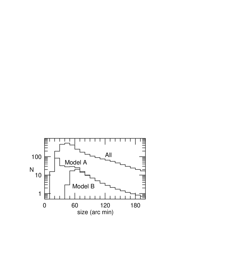
Figure 5: Expected angular size distribution of Hi SNRs.

where $A_{10}=2.86888\times 10^{-15}$ s^-1 is the spontaneous transition probability between the hyperfine structure levels of Hi, $A_{\rm eff}$ is the effective area of the telescope, and the other symbols have their usual meanings. In deriving equation (14), we assumed that the SNR size is much smaller than the telescope beam. The SNR size at the shell-formation is $2R_{\rm sf}=92.8~{}{\rm pc}=32^{\prime}\times(d/10~{}{\rm kpc})^{-1}$, and larger at later times. Hence, it appears that most Hi SNRs should have sizes larger than the beam size ($\sim 30^{\prime}$) of a 25-m telescope (cf. Fig. 5). However, the excess emission at extreme velocities that we would detect comes from small cap portions of expanding shells, and $T_{A}$ from equation (14) might yield an approximate average intensity of the emission. If the shell is thin and expands with a uniform velocity $v_{s}$, then the line profile will be a rectangular shape with velocity extent from $-v_{s}$ to $+v_{s}$, so that the left-hand side of equation (14) becomes $T_{A}\times 2v_{s}$. Hence, if the minimum detectable antenna temperature of the observation is $\Delta T_{A}$, then from equations (11) and (14), the maximum distance $d_{\rm max}(v_{s})$ is given by

$$d_{\rm max}(v_{s})={d_{\rm sf}\over\sqrt{\delta}}\left(v_{s}\over v_{\rm sf}\right)^{-1/2}\left[\left(v_{s}\over v_{\rm sf}\right)^{-9/7}-(1-\delta)\right]^{1/2},$$ (15)

where $d_{\rm sf}$ is the maximum distance at the shell-formation stage:

$$d_{\rm sf} = \left[{3hcA_{10}\over 32\pi km_{\rm H}}{A_{\rm eff}\over\Delta T_{A}}{\delta M_{\rm sf}\over 2v_{\rm sf}}\right]^{1/2}$$

$$= 1.89(A_{\rm eff,6}/\Delta T_{A,-1})^{1/2}\delta^{1/2}n_{0}^{-3/14}E_{51}^{11/28}~{}{\rm kpc},$$

with $A_{\rm eff,6}=A_{\rm eff}/(10^{6}{\rm cm}^{2})$ and $\Delta T_{A,-1}=\Delta T_{A}/(0.1~{}{\rm K})$. The probability $p_{\rm T}$ in Model B is given by

$$p_{\rm T}(x,y,v_{s})=\left\{\begin{array}[]{r@{\quad\quad}l}1&{\rm if}~{}d\leq d_{\rm max}(v_{s})\\ 0&{\rm otherwise.}\end{array}\right.$$

For a 25-m telescope with $A_{\rm eff,6}=3.0$ and $\Delta T_{A,-1}=1.0$, $d_{\rm sf}=3.5$ kpc for $n_{0}=0.14$ cm^-3 and $\delta=0.5$.

3 RESULTS

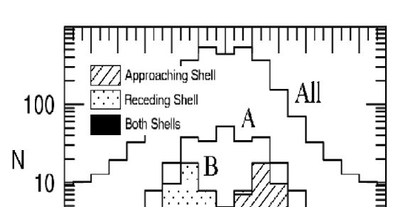
Figure 4: Expected Galactic longitude distribution of Hi SNRs. For the distribution in Model B, we mark whether the observable portions of the SNRs are approaching, receding, or both.

The basic results are shown in Fig. 2 where we plot the expected surface density distribution of Hi SNRs in the Galactic plane. Fig. 2(a) shows the distribution of all Hi SNRs, i.e., when $p_{\rm B}=p_{\rm T}=1$. The total number of Hi SNRs in our model gaseous disk is $\Sigma_{\rm SN}f_{\rm HI}\tau=2850$. This is 44% of the total ($6480$) isolated SNRs in the Galaxy. The rest are in the halo (34% or 2200) and in the central hole (22% or 1430). The distribution in Fig. 2(a) is simply due to the exponential distribution of the SN surface density. Fig. 2(b) shows the distribution of observable Hi SNRs in Model A, i.e., when $p_{\rm T}=1$. The total number of observable SNRs is now $267$, or 9.4% of the total Hi SNRs. They are concentrated along the loci of tangential points because the systematic velocities of the SNRs in those regions are close to either the maximum or the minimum velocities of the Galactic background emission. Only the receding (approaching) portion of the shell will be detectable for the Hi SNRs in the first (fourth) quadrant. The concentration near $\ell=0^{\circ}$ is because the minimum (maximum) velocity permitted by the Galactic rotation is close to zero in the first (fourth) quadrant. For those SNRs, only the approaching (receding) portion of the shell will be detectable in the first (fourth) quadrant. Near $\ell=180^{\circ}$, both the receding and approaching portions are detectable (cf. Fig. 4). Fig. 2(c) is for Model B when the observation is made with a radio telescope with an effective area of $3\times 10^{6}$ cm², which corresponds to a telescope with a diameter of 25 m, and $\Delta T_{A,-1}$=1.0. Now, the SNRs on the far side of the Galaxy are not observable and the total number is 96, or 3.4% of the total Hi SNRs.

Fig. 3 (left-hand panel) is the distribution of expansion velocities of Hi SNRs. The distribution of all Hi SNRs is given by $dN/dv_{s}\propto v_{s}^{-17/7}$ (equation 13). Among these Hi SNRs, the ones with small expansion velocities are largely unobservable because of the contamination due to the Galactic background emission, which is shown by the Model A distribution. On the other hand, the Model B distribution shows that the SNRs with large expansion velocities are largely unobservable mainly because of the limited telescope sensitivity. Fig. 3 (right-hand pannel) is the distribution of distances to Hi SNRs. The bowl between $d=5$ and 12 kpc in the distribution of all Hi SNRs is due to the central hole. The rapid drop beyond 7–8 kpc in Model A distribution is due to the small number of observable SNRs beyond tangential points in the inner Galaxy (cf. Fig. 2b). The Model B distribution shows that, with a 25-m telescope, we can detect all the observable Hi SNRs to 4 kpc and most up to 7 kpc, but no Hi SNRs beyond 9 kpc.

A statistical property that can be directly compared with the observations is the Galactic longitude distribution of Hi SNRs (Fig. 4). The distribution of all Hi SNRs peaks toward $\ell=0^{\circ}$, but not strongly because of the central hole. The background contamination brings down the real distribution by a factor of 5–16 depending on $\ell$ (Model A). The effect is largest at $\ell=10^{\circ}$–30^∘ (or 340^∘–350^∘) and smallest at $\ell=160^{\circ}$–200^∘. The telescope sensitivity further decreases the number of SNRs, most notably between $\ell=330^{\circ}$ and 30^∘ (Model B), which is understandable from Fig. 2(c). For Model B, Fig. 4 also shows whether the observable portions of the SNRs are approaching, receding, or both. Another statistical property that can be directly compared with the observations is the angular size distribution (Fig. 5). The distribution of all Hi SNRs peaks at 40^′–50^′. In the Model A distribution, there is a strong peak at 20–30^′ and a plateau between $30^{\prime}$ and 70^′. Because of the telescope sensitivity, there is no observable Hi SNRs smaller than 40^′ and the distribution peaks at 60^′–70^′ (Model B).

4 DISCUSSION

4.1 Effect of Clouds

The real ISM is pervaded by cold Hi clouds and their effect on our results should be discussed. The evolution of SNRs in a cloudy ISM has been studied numerically by Cowie et al. (1981). One of their models (model 6) is for the two-phase ISM and applicable to our case. They adopted $n_{0}=0.2$ cm^-3 and $E_{51}=0.31$, and assumed that the Spitzer’s standard Hi clouds (Spitzer, 1978) are randomly distributed with a relatively large (7%) volume filling factor (see below). They simulated the evolution until the beginning of radiative phase and showed that neither cloud evaporation nor the dynamical effects of the clouds affect the evolution of SNRs in a significant way. Their shell-formation time and radius agree with those from equations (4) and (7). They did not derive the fraction $\delta$ of mass compressed into neutral shell at the time of shell formation, but, since the interior structure is only slightly modified, we expect that $\delta$ is not significantly different from the homogeneous case, i.e., 0.5.

In radiative phase, the cloud-shell interaction depends on the ratio of their column densities. The column density of the shell of the visible Hi SNRs is (3.3–8.8)$\times 10^{18}$ cm^-2 (cf. equation 11), which is less than that of typical clouds ($\sim 1\times 10^{20}$ cm^-2). Thus, the collisions with clouds will punch holes in the shell (McKee & Ostriker, 1977; Ostriker & McKee, 1988). The hot interior gas, however, will drive a shock to reform the missing portion of the shell. Since the column density for a strong shock to be radiative $N_{\rm rad}\simeq 10^{17.5}(v_{s}/100~{}{\rm km\ s}^{-1})^{4}$ (McKee et al., 1987), the required distance for the reformation of the shell is $N_{\rm rad}/n_{0}\simeq 0.73(v_{s}/100~{}{\rm km\ s}^{-1})^{4}$ pc. This is much less than the mean distance for a particular portion of the shell to experience successive collisions (see below). Hence, in the two-phase ISM, the Hi SNRs will be punched by cold clouds as they expand, but the holes will be quickly recovered. The shell loses mass and momentum by the collision with clouds.

The evolution of such radiative SNRs in cloudy medium has been analyzed by Ostriker & McKee (1988). The key factor that determines the importance of clouds is $\exp[-(R_{s}-R_{\rm sf})/\lambda_{\rm cl}]$ where $\lambda_{\rm cl}$ is the cloud mean free path. For example, the mass in the shell at the time of shell formation decreases by this factor due to the collisions with clouds as it expands. If $(R_{s}-R_{\rm sf})/\lambda_{\rm cl}\ll 1$, therefore, the ‘cloud-punching’ is not important. If the clouds are spherical with radius $a_{\rm cl}$ and their volume filling factor is $f_{\rm cl}$, then $\lambda_{\rm cl}=(4/3)a_{\rm cl}/f_{\rm cl}$. The filling factor of cold clouds can be inferred from their characteristic and space-averaged densities. The two-phase equilibrium yields the density of cold clouds $n_{\rm cl}\simeq 40$ cm^-3, which agrees with observations (McKee, 1995). The space-averaged density of cold Hi near the Sun is $\simeq 0.3$ cm^-3 (e.g., Ferriére, 1995), so that $f_{\rm cl}\simeq 0.3/40=0.75$%. The characteristic radius of the clouds inferred from the Hi column density ($N_{\rm cl}=4\times 10^{20}$ cm^-2) of ‘standard’ Hi clouds (Spitzer, 1978) is $a_{\rm cl}=(3/4)N_{\rm cl}/n_{\rm cl}=2.4$ pc. Therefore, $\lambda_{\rm cl}\simeq 430$ pc and $(R_{s}-R_{\rm sf})/\lambda_{\rm cl}\leq 5.7\times 10^{-2}$ for visible Hi SNRs. This implies that the cloud punching effect is not important for the evolution of visible Hi SNRs and therefore for their statistics.

Recently Heiles & Troland (2003) showed that in two regions they studied the cold ISM is distributed in huge blobby sheets of thickness $\sim 0.11$ and $\lower 2.15277pt\hbox{$\;\buildrel<\over{\sim}\;$}3.6$ pc with lengh-to-thickness aspect ratios $\sim 280$ and $\sim 70$, and, proposed that, if these characteristics are general, the cold ISM could be organized into a small number of large sheetlike structures instead of a large number of randomly distributed small clumps. If the ISM morphology is close to this clumpy sheet model, then the probability for a SNR to cross the sheets will be small and only a portion of the SNR will be affected by the interaction, so that the the statistics of Hi SNRs will be determined by the nature of the intercloud medium.

4.2 Comparison with Observation

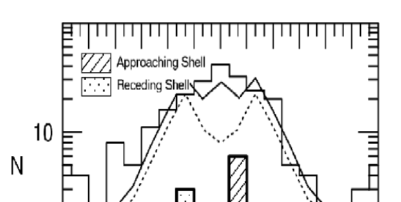
Figure 6: Galactic longitude distribution of SNRs. The distribution of the observed Hi SNR candidates is shown by a thick histogram, where we mark whether their approaching or receding portions are detected. For comparison, the expected distributions for the parameters of KH91 and Koo et al. (2003) are shown by solid and dotted lines, respectively. The distribution of all known 231 SNRs is also shown as a thin histogram.

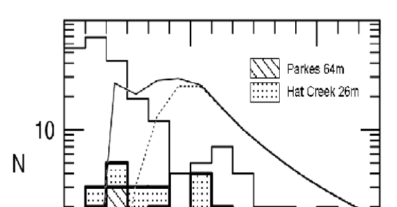
Figure 7: Angular size distribution of SNRs. The meanings of curves and histograms are same as those of Fig. 6. For the distribution of the Hi SNR candidates, we mark the contributions from the northern (Hat Creek 26m) and southern (Parkes 64m) sky surveys, separately.

Our results can be compared with results of KH91 and Koo et al. (2003) introduced in Section 1. In short, KH91 did a sensitive survey of Hi 21 cm emission lines toward 103 northern Galactic SNRs using the Hat Creek 26-m telescope ($A_{\rm eff}\simeq 3.0$), and detected faint extended wing at forbidden velocities toward 15 SNRs. The sensitivity (1.5$\sigma$) of the survey was $\sim 0.06$ K. Koo et al. (2003) searched for similar Hi features toward 97 southern SNRs and identified another 10 SNRs. The Southern Galactic Plane Survey data was obtained with the Parkes 64-m telescope ($A_{\rm eff,6}=18$). The sensitivity ($1.5\sigma$) of the survey was 0.09–0.14 K. These 25 (=15+10) SNRs constitute the Hi SNR candidates (see comment in Section 1). On the other hand, the expected number from Model B for the parameters of KH91, e.g., $A_{\rm eff,6}/\Delta T_{A,-1}=3.0/0.6=5$, is $\simeq 120$, and for those of Koo et al. (2003) is $\simeq$190–220. Therefore, the observed number of Hi SNRs is less than the expected by a factor of $\lower 2.15277pt\hbox{$\;\buildrel>\over{\sim}\;$}5$. Fig. 6 shows the Galactic longitude distribution of the Hi SNR candidates. For comparison, we show the expected distributions and also the distribution of all known Galactic SNRs in the Green’s catalog (Green 2001). Most candidates in the first quadrant have an excess emission at positive velocities, while those in the fourth quadrant at negative velocities. This seems to be consistent with our expectation (Fig. 4). Fig. 7 shows the angular size distribution. Most (72%) Galactic SNRs have sizes smaller than 30^′, while the average size of Hi SNR candidates is $46^{\prime}$. A significant (36%) fraction of Hi SNR candidates has size less than $30^{\prime}$ whereas none is expected from the model.

The discrepancy between the observed and the expected numbers is significant and needs to be explained. A plausible explanation is that the old SNRs are too faint to be identified in radio continuum, so that the Hi surveys by KH91 and Koo et al. (2003), which were based on the current (radio continuum-based) SNR catalog, might have missed most of the SNRs with Hi shells. This thought led us to search for Hi SNRs based on the Hi data. We used the Leiden-Dwingeloo (LD) Hi survey data, which was obtained by Hartmann & Burton (1997) using the Dwingeloo 25-m radio telescope (HPBW=36^′). The survey covers the Galactic plane ($|b|\lower 2.15277pt\hbox{$\;\buildrel<\over{\sim}\;$}10^{\circ}$) between $\ell=0^{\circ}$ and 260^∘, and the rms sensitivity of the final data cube is 0.07 K. We first examined about 130 SNRs in the Green’s catalogue and have found high-velocity features toward $\leq 10$ SNRs. These SNRs look protruding from their surroundings in ($\ell$, $v$) diagram (cf. Fig. 1). We then examined individual ($\ell,v$) maps with the naked eye, and have identified $\sim 70$ similar-looking, forbidden-velocity features not related to the known SNRs. Fig. 8 is an example where we can see several such features. Some of these “forbidden-velocity (FV) wings” are associated with galaxies or perhaps HII regions, but most (70%) of them are not. Could they be the so-far undiscovered old Hi SNRs? We have been looking into these regions in various wavelengths, but have not identified their natures yet. But the distribution of FV wings appears to be very different from the expected distribution of visible Hi SNRs (Fig. 9): Between $\ell=0^{\circ}$ and 70^∘, the number of FV wings is much less than the expected number of Hi SNRs, while, between $\ell=70^{\circ}$ and $250^{\circ}$, it is significantly greater in general. Possible candidates for such extended forbidden-velocity Hi wings other than SNRs are stellar wind-blown shells, neutral stellar winds associated with protostars (Lizano et al., 1988), high-velocity and/or intermediate clouds, galaxies, etc. The detailed results are in preparation (Kang et al., 2003).

If the observed number ($\leq 25$) turns out to be close to the total number of Hi SNRs in the Galaxy, then the discrepancy implies that either some of our input parameters are inaccurate or some of our basic assumptions are wrong. The parameters and assumptions regarding the frequency and distribution of SNe, however, are chosen to minimize the number of Hi SNRs when they are uncertain, e.g., we have assumed that all core-collapse SNe explode in groups and only SNe Ia produce isolated SNRs. The total SN Ia rate cannot be much lower than what we adopted ($0.45\times 10^{-2}$) if we consider that there are at least two SN Ia (Tycho and SN 1006) during last 2,000 years in the solar neighborhood. We have discussed the effect of magnetic fields, thermal conduction, and embedded clouds on the evolution of SNRs in Sections 2.3 and 4.1, and concluded that they are not dynamically important for the visible Hi SNRs which are moving fast. If the Hi disk is denser and thinner, the number of visible Hi SNRs will decrease, but not by a large factor. For example, if the density of the Hi disk is $\sim 0.5$ cm^-3 and its thickness is $\sim 200$ pc, the number decreases by $\sim 40$%. One possibility is that the interstellar space in the inner Galaxy is not filled with WNM, but mostly filled with a very hot, diffuse ($3.5\times 10^{-3}$ cm^-3) medium as in the three phase model of McKee & Ostriker (1977). In such a tenuous medium, the SNRs develop dense shells when they are very old ($9\times 10^{5}$ yr, equation 4), at which time their radius is 230 pc. But this radius is very large, so that it is possible that the SNRs come into equilibrium with the interstellar pressure or overlap with other SNRs before dense shell formation, in which case Hi shells are not formed (McKee & Ostriker, 1977). Embedded clouds could be accelerated by the SNR shock and also by the ram pressure, but numerical simulations by Cowie et al. (1981) showed that they are substantially destroyed by evaporation before acquiring high velocities. In the three-phase ISM, the observed Hi SNRs may be the ones in special environments, e.g., near large atomic or molecular clouds.

The above conclusion on the structure of the ISM in the inner Galaxy would not be totally changed even if the FV wing sources turn out to be Hi SNRs because, according to Fig. 9, there are much less number of FV wings than what the model predicts in the inner Galaxy. In the outer Galaxy, however, the number is significantly greater than the predicted. The model distribution can be made to have more Hi SNRs in the outer Galaxy, for example, by increasing the radial scale length of SNe distribution, but it cannot be made to be consistent with the observed FV wing distribution simply by changing some of its parameters. We postpone further discussion on the FV wings and their significance after identifying their natures.

5 SUMMARY

We have developed a simple model to estimate the number of old, radiative SNRs visible in Hi 21-cm emission line in the Galaxy. Old SNRs are expected to be surrounded by rapidly expanding Hi shells, but the contamination due to the Galactic background Hi emission severely limits their visibility. The visible SNRs are defined as the ones with a sufficiently large expansion velocity, so that their line-of-sight velocities are significantly ($\geq 50$ km s^-1) outside the velocity range of the Galactic background Hi emission. Another factor that determines the visibility is the telescope sensitivity, which is included in our formulation. Some of the essential features of our model are (1) the Hi gas in the Galaxy is confined to an axi-symmetric, center-emptied disk with an inner edge at 3.5 kpc and outer edge at 15 kpc, (2) the Hi disk is uniform and homogeneous, and the density of the disk is $0.14$ cm^-3, (3) the disk is rotating with a constant speed $v_{\odot}=220$ km s^-1, (4) only SNe Ia produce isolated SNRs, (5) total Galactic SN Ia rate is $0.45\times 10^{-2}$ yr^-1, but only 44% of them explodes within the gaseous disk to produce Hi SNRs (34% explodes above and below the disk while 22% within the central hole), and (6) the SNe Ia are exponentially distributed with a radial scale length of 3 kpc. We use the equations of Cioffi et al. (1988) in a slightly modified form to calculate how the radius, velocity, and mass of a SNR shell vary with time, and, at each position in the disk, we derive the number of visible SNRs.

According to our result, the number of Hi SNRs in the Galaxy is 2850. Galactic background contamination limits the number of visible SNRs to $\simeq 270$, or $\simeq 9$% of the total Hi SNRs. They are concentrated along the loci of tangential points and near $\ell=0^{\circ}$ (Fig. 2b). The telescope sensitivity may prevent observing the ones on the far side of the Galaxy (Fig. 2c). We have calculated the expected number of visible Hi SNRs for realistic observational parameters and compared the results with observations. There have been two systematic Hi 21-cm emission line studies toward 103 northern and 97 southern SNRs, and faint extended wings at forbidden velocities have been detected toward 25 SNRs (KH91; Koo et al., 2003). The expected number is much ($\lower 2.15277pt\hbox{$\;\buildrel>\over{\sim}\;$}5$) greater than this.

We consider that our estimate is on the conservative side and the discrepancy is significant. A plausible explanation is that previous observational studies, which were made toward the SNRs identified in radio continuum, missed most of the Hi SNRs because they are too faint to be visible in radio continuum. We propose that the faint extended wings at forbidden velocities seen in Hi 21-cm line surveys (e.g., Fig. 8) could be possible candidates for such old Hi SNRs. According to our our preliminary result, however, their Galactic longitude distribution is quite different from the expected distribution of visible Hi SNRs, e.g., the number of FV wings is considerably less than the expected in the inner Galaxy. The natures of the FV wings need to be identified. If the observed number ($\leq 25$) turns out to be close to the total number of Hi SNRs in the Galaxy, then the discrepancy implies that either some of our input parameters are inaccurate or some of our basic assumptions are wrong. A possible explanation is that the interstellar space in the inner Galaxy is largely filled with a very tenuous gas as in the three-phase ISM model. In this case, the observed Hi SNRs are likely the ones in special environments, e.g., near large atomic or molecular clouds.

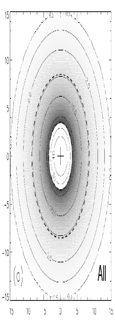
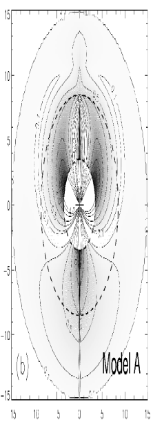
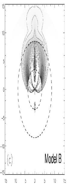
Figure 2: Expected surface density (kpc^-2) distribution of (a) all Hi SNRs ($p_{\rm B}=p_{\rm T}=1$), (b) observable Hi SNRs in Model A ($p_{\rm T}=1$), and (c) observable Hi SNRs in Model B ($A_{\rm eff,6}/\Delta T_{A,-1}=3.0$). The inner and outer circles marked by dashed lines are at $r=3.5$ kpc and 8.5 kpc, respectively. In our model, the region inside the inner circle is devoid of the ISM and there the SNe explosion do not produce Hi SNRs.

Figure 3: Expected distribution of Hi SNRs in: (left-hand panel) expansion velocities; (right-hand panel) distances.

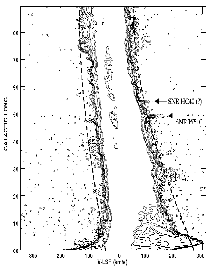
Figure 8: ($\ell,v$) diagram of Hi 21-cm emission at $b=-0.^{\circ}5$. Contour levels start at 0.1 K and end at 10 K. Note the spatially-confined, faint extended wings at forbidden velocities (FV wings). Some of them are associated with SNRs, e.g., the one between $v_{\rm LSR}=80$ and 140 km s^-1 near $\ell=49^{\circ}$ (SNR W51C) and also, possibly, the one between $v_{\rm LSR}=80$ and 110 km s^-1 near $\ell=54^{\circ}$ (SNR HC 40). But the others are not related to the known SNRs. The dashed lines are the same as those in Fig. 1.

Figure 9: Galactic longitude distribution of FV wings compared to the expected distribution of Hi SNRs.

References

- Assousa & Erkes (1973) Assousa, G. E., & Erkes, J. W. 1973, AJ, 78, 885
- Binney & Merrifield (1998) Binney, J., & Merrifield, M. 1998, Galactic Astronomy (Princeton: Princeton Univ. Press)
- Blondin et al. (1998) Blondin, J. M., Wright, E. B., Borkowski, K. J., & Reynolds, S. P. 1998, ApJ, 500, 342
- Braun & Strom (1986) Braun, R., & Strom, R. G. 1986, A&AS, 63, 345
- Cappellaro et al. (1999) Cappellaro, E., Evans, R., & Turatto, M. 1999, A&A, 351, 459
- Chevalier (1974) Chevalier, R. A. 1974, ApJ, 188, 501
- Cioffi et al. (1988) Cioffi, D. F., McKee, C. F., & Bertschinger, E. 1988, ApJ, 334, 252
- Colomb & Dubner (1980) Colomb, F. R., & Dubner, G. 1980, A&A, 82, 244
- Colomb & Dubner (1982) ——. 1982, A&A, 112, 141
- Cowie et al. (1981) Cowie, L. L., McKee, C. F., & Ostriker, J. P. 1981, ApJ, 247, 908
- Cox (1972) Cox, D. P. 1972, ApJ, 178, 159
- Dawson, & Johnson (1994) Dawson, P. C., & Johnson, R. G. 1994, J. R. Astron. Soc. Can., 88, 369
- DeNoyer (1978) DeNoyer, L. K. 1978, MNRAS, 183, 187
- Dickey & Lockman (1990) Dickey, J. M., & Lockman, F. J. 1990, ARAA, 28, 215
- Drimmel, & Spergel (2001) Drimmel, R., & Spergel, D. N. 2001, ApJ, 556, 181
- Falle (1981) Falle, S. A. E. G. 1981, MNRAS, 195, 1011
- Ferriére (1995) Ferriére, K. M. 1995, ApJ, 441, 281
- Field et al. (1969) Field, G. B., Goldsmith, D., & Habing, H. 1969, ApJ, 15, L49
- Freudenreich (1998) Freudenreich, H. T. 1998, ApJ, 492, 495
- Gies (1987) Gies, D. R. 1987, ApJS, 64, 545
- Gies & Bolton (1986) Gies, D. R., & Bolton, C. T. 1986, ApJS, 61, 419
- Giovanelli & Haynes (1979) Giovanelli, R., & Haynes, M. P. 1979, ApJ, 230, 404
- Green (2001) Green, D. A. 2001, ‘A Catalogue of Galactic Supernova Remnants (2001 December version)’, Mullard Radio Astronomy Observatory, Cavendish Laboratory, Cambridge, United Kingdom (available on the World-Wide-Web at ”http://www.mrao.cam.ac.uk/surveys/snrs/”)
- Hartmann & Burton (1997) Hartmann, D., & Burton, W. B. 1997, Atlas of Galactic Neutral Hydrogen (Cambridge: Cambridge Univ. Press)
- Hatano et al. (1998) Hatano, K., Branch, D., & Deaton, J. 1998, ApJ, 502, 177
- Heiles (1987) Heiles, C. 1987, ApJ, 315, 555
- Heiles & Troland (2003) Heiles, C., & Troland, T. H. 2003, ApJ, 586, 1067
- Humphreys & McElroy (1984) Humphreys, R. M., & McElroy, D. B. 1984, ApJ, 284, 565
- Kang et al. (2003) Kang, J., Koo, B.-C., & Heiles, C. 2003, in preparation
- Kent et al. (1991) Kent, S. M., Dame, T. M., & Fazio, G. 1991, ApJ, 378, 131
- Kimoto & Chernoff (1997) Kimoto, P. A., & Chernoff, D. F. 1997, ApJ, 485, 274
- Knapp & Kerr (1974) Knapp, G. R., & Kerr, F. J. 1974, A&A, 33, 463
- Koo (2003) Koo, B.-C. 2003 in ASP Conf. Ser. 289, IAU 8th Asian-Pacific Regional Meeting Proceedings Volume I, ed. S. Ikeuchi, J. Hearnshaw, & T. Hanawa (San Francisco: ASP), 199
- Koo & Heiles (1991) Koo, B.-C., & Heiles, C. 1991, ApJ, 382, 204
- Koo & Heiles (1995) Koo, B.-C., & Heiles, C. 1995, ApJ, 442, 679
- Koo et al. (2003) Koo, B.-C., Kang, J., & McClure-Griffiths, N. M. 2003, in preparation
- Koo & Moon (1997) Koo, B.-C., & Moon, D.-S. 1997, ApJ, 475, 194
- Koo et al. (1990) Koo, B.-C., Reach, W. T., Heiles, C., Fesen, R. A., & Shull, J. M. 1990, ApJ, 364, 178
- Kulkarni et al. (1982) Kulkarni, S. R., Blitz, L., & Heiles, C. 1982, ApJ, 259, L63
- Kulkarni & Heiles (1987) Kulkarni, S. R., & Heiles, C. 1987, in Interstellar Processes, ed. D. J. Hollenbach & H. A. Thronson, Jr. (Dordrecht: D. Reidel) 87
- Landecker et al. (1980) Landecker, T. L., Roger, R. S., & Higgs, L. A. 1980, A&AS, 39, 133
- Lizano et al. (1988) Lizano, S., Heiles, C., Rodríguez, L. F., Koo, B.-C., Shu, F., H., Hasegawa, T., Hayashi, S., & Mirabel, I. F. 1988, ApJ, 328, 763
- Lockman (1984) Lockman, F. J. 1984, ApJ, 283, 90
- López-Corredoira et al. (2002) López-Corredoira, M., Cabrera-Lavers, A., Garzón, F., & Hammersley, P. L. 2002, A&A, 394, 883
- Mansfield & Salpeter (1974) Mansfield, V. N., & Salpeter, E. E. 1974, ApJ, 190, 305
- McClure-Griffiths (2001) McClure-Griffiths, N. 2001, PhD thesis (University of Minnesota)
- McKee (1990) McKee, C. F. 1990 in ASP Conf. Ser. 12, The Evolution of the Interstellar Medium, ed. L. Blitz (San Francisco: ASP), 3
- McKee (1995) McKee, C. F. 1995 in ASP Conf. Ser. 80, The Physics of the Interstellar Medium and Intergalactic Medium, ed. A. Ferrara, C. F. McKee, C. Heiles, & P. R. Shapiro (San Francisco: ASP), 292
- McKee et al. (1987) McKee, C. F., Hollenbach, D. J., Seab, C. G., & Tielens, A. G. G. M. 1987, ApJ, 318, 674
- McKee & Ostriker (1977) McKee, C. F., & Ostriker, J. P. 1977, ApJ, 218, 148
- McKee et al. (1984) McKee, C. F., Van Buren, D., & Lazareff, B. 1984, ApJ, 278, L115
- Mdzinarishvilli & Dzigvashvilli (2001) Mdzinarishvilli, T., & Dzigvashvilli, R. 2001, Astrophysics, 44, 463
- Ojha (2001) Ojha, D. K. 2001, MNRAS, 322, 426
- Ostriker & McKee (1988) Ostriker, J. P., & McKee, C. F. 1988, Rev. Mod. Phys., 60, 1
- Slavin & Cox (1992) Slavin, J. D., & Cox, D. P. 1992, ApJ, 392, 131
- Spitzer (1978) Spitzer, L. I. 1978, Physical Processes in the Interstellar Medium (New York: Wiley)
- Trimble (2000) Trimble, V. 2000, in Allen’s Astrophysical Quantities, ed. A. N. Cox (New York: AIP Press)
- van den Bergh (1988) van den Bergh, S. 1988, Comments Astrophys., 12, 131
- van den Bergh (1997) van den Bergh, S. 1997, AJ, 113, 197
- van den Bergh & Tammann (1991) van den Bergh, S., & Tammann, G. A. 1991, ARA&A, 29, 363
- van den Bergh & McClure (1994) van den Bergh, S., & McClure, R. D. 1994, ApJ, 425, 205
- Wang et al. (1997) Wang, L., Höflich, P., & Wheeler, J. C. 1997, ApJ, 483, L29