Coronal Heating and Acceleration of the High/Low-Speed Solar Wind by Fast/Slow MHD Shock Trains

Abstract

We investigate coronal heating and acceleration of the high- and low-speed solar wind in the open field region by dissipation of fast and slow magnetohydrodynamical (MHD) waves through MHD shocks. Linearly polarized Alfvén (fast MHD) waves and acoustic (slow MHD) waves travelling upwardly along with a magnetic field line eventually form fast switch-on shock trains and hydrodynamical shock trains (N-waves) respectively to heat and accelerate the plasma. We determine one dimensional structure of the corona from the bottom of the transition region (TR) to 1AU under the steady-state condition by solving evolutionary equations for the shock amplitudes simultaneously with the momentum and proton/electron energy equations. Our model reproduces the overall trend of the high-speed wind from the polar holes and the low-speed wind from the mid- to low-latitude streamer except the observed hot corona in the streamer. The heating from the slow waves is effective in the low corona to increase the density there, and plays an important role in the formation of the dense low-speed wind. On the other hand, the fast waves can carry a sizable energy to the upper level to heat the outer corona and accelerate the high-speed wind effectively. We also study dependency on field strength, $B_{0}$, at the bottom of the TR and non-radial expansion of a flow tube, $f_{\rm max}$, to find that large $B_{0}/f_{\rm max}\;\buildrel>\over{\sim}\;2$ but small $B_{0}\simeq 2$G are favorable for the high-speed wind and that small $B_{0}/f_{\rm max}\simeq 1$ is required for the low-speed wind.

1 Introduction

The problems of the coronal heating and the solar wind acceleration should be investigated simultaneously since they are very closely related, although they have been often discussed separately. Even combined models, taking into account them together, usually adopt too simplified heating and acceleration law: they adopt unspecified mechanical energy and momentum inputs of the exponential type, $\propto\exp(\frac{-(r-R_{\odot})}{l_{\rm m}})$, with an assumed constant dissipation length, $l_{\rm m}$, for lack of an alternative (e.g.Sandbæk & Leer 1994), although the constant $l_{\rm m}$ is poorly supported by fundamental physical processes. Therefore, it is required to treat the energy transfer and momentum transfer simultaneously in the broad corona including the solar wind with realistic heating and acceleration functions.

The origin of the energy to heat the corona and accelerate the solar wind is generally believed to lie in the turbulent convective motions beneath the photosphere. The major difficulties in understanding the problems are how to lift up the energy to the corona and let it dissipate at the appropriate locations. Various modes of waves are supposed to play important roles in these processes (see Roberts 2000 for recent review). Not only the surface granulations but also dynamical activities such as the small magnetic reconnection events (Tsuneta, 1996; Tarbell, Ryutova, & Covington, 1999; Sakai et al., 2000; Katsukawa & Tsuneta, 2001) excites the waves from at the photospheric level to in the corona (Sturrock, 1999). MHD waves have been studies long as reliable heating and acceleration sources of the solar coronal plasma (e.g. Barnes 1969; Belcher 1971). Many groups have examined advanced properties on the wave propagation and damping such as non-WKB effects (MacGregor & Charbonneau, 1994; Ofman & Davila, 1998), steepening of slow (Ofman, Nakariakov, & Shegal, 2000) and fast (Nakariakov, Ofman & Arber, 2000) MHD waves, and shock formation (Hollweg, 1992) to study the wave heating. As an effect beyond the MHD, resonant dissipation of ion-cyclotron waves (Dusenbery & Hollweg, 1981; Marsch, Coertz, & Richter, 1982) has also been highlighted as a heating source of the heavy ions in the high-speed solar wind (Cranmer, Field, & Kohl, 1999; Hu & Habbal, 1999). However, because of the too high resonant frequencies, the protons and electrons, underlying the coronal plasma, are expected to be mainly heated by the MHD waves with lower frequency in which the most of the wave energy is contained. Signatures of such MHD waves have been observed in various portions of the solar corona (Hassler et al., 1990; Banerjee et al., 1998; Ofman, Nakariakov, & DeDorest, 1999; O’Shea, Mulglach, & Fleck, 2002), whereas dominant processes in the wave heating yet remain to be determined.

When one considers the MHD waves travelling along with a magnetic field line in the low-$\beta$ plasma, they can be divided in two types in the linear regime where the wave amplitude is sufficiently smaller than the phase speed. One is slow-mode wave which is longitudinal wave and essentially identical to the acoustic wave. The other is Alfvén wave which is transverse wave. When the non-linear terms are taken into account, the degeneracy of the transverse waves is removed; they can be divided into circularly polarized Alfvén wave classified as the MHD intermediate-mode, and linearly polarized Alfvén wave classified as the MHD fast-mode. Among these three types of the MHD waves, the fast-mode and slow-mode waves nonlinearly steepen their shapes through propagation to eventually form the MHD fast shocks and slow shocks respectively. Suzuki (2002; hereafter S02) investigated the dissipation of the N-wave which is a special case of the slow-shock trains propagating along the field line. S02 also inspected the consequent heating in self-consistent modelling to conclude that the N-waves can heat the inner corona effectively though they cannot heat the entire corona. The heating by the dissipation of the switch-on shock trains, a special case of the fast shock trains, was proposed by Hollweg (1982; hereafter H82). He studied the problem on fixed coronal structures to conclude that it can be a reliable process of the coronal heating. However, the self-consistent treatment of their propagation and dissipation has not been performed so far.

In this paper, we investigate the coronal heating and the solar wind acceleration by the switch-on shock trains as well as the N-waves in a self-consistent manner. First, by extending the formulation introduced by H82, we derive an equation describing variation of the switch-on shock trains in the similar way to that adopted by Stein & Schwartz (1972) and S02 for the N-waves. We solve these equations for the shock trains simultaneously with the equations of the momentum transfer and energy transfer to determine the unique structure of the corona and solar wind from the bottom of the transition region (TR) to 1AU for given wave energy flux of the linearly polarized Alfvén waves, $F_{\rm w,\perp,0}$, and acoustic waves, $F_{\rm w,\parallel,0}$, at the coronal base. The heating and the acceleration by the dissipation of the shock trains are explicitly taken into account. Therefore, we do not have to take the phenomenological approach adopting the exponential type of the heating law. Conversely, we can test the validity of the assumption of the constant dissipation length for our processes.

We further explore possibilities whether our model can account for the difference between the high-speed solar wind ($\;\buildrel>\over{\sim}\;700$km/s) from the polar coronal holes and the low-speed solar wind ($\;\buildrel<\over{\sim}\;400$km/s) in the equatorial region during the low solar activity phase. We adopt various field strength at the bottom of the TR and non-radial expansion factor as well as $F_{\rm w,\perp,0}$ and $F_{\rm w,\parallel,0}$ to study which parameter plays a role in exhibiting the distinctive difference between the two types of the solar wind.

2 Variation of Shock Amplitude

2.1 N-waves

Acoustic waves have not been considered as a major heating source of the solar corona for several decades, because those generated by the granule motions at photospheric level cannot reach the corona (Stein & Schwartz, 1972). However, recent observations have revealed dynamical natures of the corona; a lot of transient events such as microflares constantly occur. Some models (Sturrock, 1999; Kudoh & Shibata, 1999) describing those events predict excitation of acoustic waves, or equivalently slow-mode MHD waves, not at the photosphere but in the corona. Moreover, Ofman et al.(1999) identified slow MHD waves propagating in polar plumes. If one considers such waves travelling along with the magnetic field line in the open flux tube region, they eventually form shocks and propagate upwardly as the N-waves (Fig.1), a special case of the slow-shock trains, with heating the surrounding plasma. For example, the waves of sinusoidal shape with period, $\tau_{\parallel}\sim 100$s, steepen their wave fronts to form the shocks after propagation by a distance of $\sim 10^{4}$km in the corona, provided that the initial wave amplitude is $\;\buildrel>\over{\sim}\;10$% of the sound speed (S02).

A model for the N-waves was developped for propagation in the chromosphere by Stein & Schwartz (1972), and generalized for propagation in the corona by S02. Now, we briefly summarize the derivation of an equation for variation of amplitude of the N-waves by following S02. We assume the shock amplitude, $\delta v_{\rm sh,\parallel}$, is sufficiently smaller than ambient sound speed, $c_{\rm s}$ (weak-shock approximation). Then, entropy generation at each shock front is given by the jump condition across the shock as

$$\frac{\Delta s_{\parallel}}{R}=\frac{\gamma+1}{12\gamma^{2}}(\frac{\Delta p}{p})^{3}=\frac{2\gamma(\gamma+1)}{3}\alpha_{\rm sh,\parallel}^{3},$$ (1)

(Landau & Lifshitz, 1959), where $R$ is the gas constant, $\gamma$ is a ratio of the specific heat, $\Delta p$ denotes pressure difference at the front, $p$ is pressure in the upstream region, and $\alpha_{\rm sh,\parallel}(\equiv\delta_{\rm sh,\parallel}/c_{\rm s})$ is the normalized shock amplitude. Using the perfect gas law, $T=p/(\rho R)$, the energy loss rate $-Q_{\parallel}$ per volume (erg cm^-3s^-1) at the shocks for the waves with period $\tau_{\parallel}$ is derived from eq. (1):

$$-Q_{\parallel}=-\rho_{0}T\Delta s_{\parallel}/\tau_{\parallel}=-\frac{2\gamma(\gamma+1)p_{0}\alpha_{\rm sh,\parallel}^{3}}{3\tau_{\parallel}}.$$ (2)

Divergence of wave energy, $E_{\lambda_{\parallel}}=\frac{1}{\varsigma_{\parallel}}\gamma p\alpha_{\rm sh,\parallel}^{3}\lambda_{\parallel}$, per wavelength, $\lambda_{\parallel}$, for a shape constant, $\varsigma_{\parallel}$($=3$ for the N-waves illustrated in Fig.1), can be written as

$$\mbox{\boldmath${\nabla\cdot E_{\lambda_{\parallel}}}$}=\frac{dE_{\lambda_{\parallel}}}{dr}+\frac{E_{\lambda_{\parallel}}}{A}\frac{dA}{dr}=-Q_{\parallel}\tau_{\parallel},$$ (3)

where $A$ is a cross section of a flow tube. Substitution of eq.(3) into the logarithmic derivative of $E_{\lambda_{\parallel}}$ gives variation of the shock amplitude in the static media as follows (S02) :

$$\frac{d\alpha_{\rm sh,\parallel}}{dr}=\frac{\alpha_{\rm sh,\parallel}}{2}(-\frac{1}{\rho}\frac{d\rho}{dr}-\frac{\varsigma_{\parallel}}{3}\frac{2(\gamma+1)\alpha_{\rm sh,\parallel}}{c_{\rm s}\tau_{\parallel}}-\frac{1}{A}\frac{dA}{dr}-\frac{3}{c_{\rm s}}\frac{dc_{\rm s}}{dr}).$$ (4)

This equation determines the variation of the shock amplitude of the N-waves in the solar corona according to the physical properties of the background coronal plasma. The first term in the right-hand side denotes the amplification in the stratified atmosphere, and the second term indicates the loss by the shock heating. In the $(1-2)R_{\odot}$ region, where the dissipation is important to heat the corona, these two terms always dominate the other terms, the third term arising from the geometrical expansion and the fourth from temperature variation.

Figure 1: Schematic picture of the steepening of acoustic waves (top) and linearly polarized Alfvén waves (bottom).

2.2 Switch-on Shock Trains

The various dynamical activities on the solar surface are expected to continuously produce transverse waves. Some of them would be linearly polarized Alfvén waves propagating upwardly. Phase speed of the linearly polarized Alfvén waves varies as a function of fluctuating field, $\delta B_{\perp}$, normal to the background field, $B_{\parallel}$(Kulikovskiy & Lyubimov, 1965):

$$v_{\rm p}=\frac{\sqrt{B_{\parallel}^{2}+\delta B_{\perp}^{2}}}{\sqrt{4\pi\rho}}.$$ (5)

The above equation also satisfies the requirement of the plasma compressibility (Montgomery, 1959),

$$\frac{(B_{\parallel}^{2}+\delta B_{\perp}^{2})^{1/2}}{\rho}\simeq{\rm const.}$$ (6)

Equations (5) and (6) shows that both the wave crest and the wave trough overtake the wave front with a speed,

$$\frac{\sqrt{B_{\parallel}^{2}+\delta B_{\perp}^{2}}}{\sqrt{4\pi\rho}}-\frac{B_{\parallel}}{\sqrt{4\pi\rho_{0}}}=v_{\rm A}[(\frac{B_{\parallel}^{2}+\delta B_{\perp}^{2}}{B_{\parallel}^{2}})^{\frac{1}{4}}-1],$$ (7)

where we here define Alfvén velocity, $v_{\rm A}\equiv B_{\parallel}/\sqrt{4\pi\rho_{0}}$ for the ambient density $\rho_{0}$ at the wave fronts. Then two shock fronts are formed per wavelength as illustrated in Fig. 1, which is also seen in results of time-dependent calculations by Nakariakov et al.(2000). The figure also displays that as moving from the upstream region to the downstream region, $\delta B_{\perp}$ and $\delta v_{\perp}$ ’switch-on’ from zero to finite values. Therefore, it is called switch-on shock, a special case of the fast shocks. Periodic trains of the switch-on shocks propagate upwardly with a speed $\simeq v_{\rm A}$, similarly to the usual Alfvén waves except that they dissipate the wave energy at each shock.

Let us estimate a distance the sinusoidal wave travels till the formation of the shock fronts. We can categorize these transverse waves into two types in terms of location of the wave generation. First type is the wave generated by the granule motions at the photosphere. Since the Alfvén velocity in the photosphere and low chromosphere is quite small, the sinusoidal waves steepen to form the shock trains before reaching the corona. This is seen in recent time-dependent calculation by Kudoh & Shibata (1999), illustrating that the transverse waves created at the photosphere propagate into the corona as the fast shocks.

Second type is the wave excited by transient events such as microflares in the corona. To form the front, the wave crest or trough have to overtake the wave front by a quarter of a wave length, $\lambda_{\perp}$. If we set that the sinusoidal waves are generated at time $t_{0}$ and position $R_{0}$, time $t$ and position $R$, at which the waves steepen to form the fronts, satisfy the conditions below in a static atmosphere.

$$\int_{t_{0}}^{t}dt^{\prime}v_{\rm A}[(\frac{B_{\parallel}^{2}+\delta B_{\perp}^{2}}{B_{\parallel}^{2}})^{\frac{1}{4}}-1]=\int_{R_{0}}^{R}dr[(\frac{B_{\parallel}^{2}+\delta B_{\perp}^{2}}{B_{\parallel}^{2}})^{\frac{1}{4}}-1]=\frac{\lambda_{\perp}}{4}$$ (8)

If we consider wave with period, $\tau_{\perp}=120$s, generated at $R_{0}=R_{\odot}+1\times 10^{4}$km, substitution of typical values in the corona of $B_{\parallel}\sim 5$G, $\delta B_{\perp}\sim 1$G, and density scale height, $H\simeq 6\times 10^{4}(\frac{T}{10^{6}{\rm K}})$km, into eq.(8) gives $R\simeq 1.3R_{\odot}$. It indicates that even if the linearly polarized Alfvén waves are excited in the corona, they form the fast shocks in the low corona. Moreover, the assumption of the generation of the sinusoidal waves is idealistic and the initial wave shape is supposed to be more or less out of shape in the real solar corona. In a such case the distance till the formation of the shocks should become shorter.

From now, we would like to derive an equation describing variation of amplitude of the switch-on shock trains by extending the formulation by H82. From the jump conditions across the switch-on shock front (Boyd & Sanderson, 1969), entropy generation $\Delta s_{\perp}$ at the shock can be expressed as

$$\frac{\Delta s_{\perp}}{R}\simeq\frac{B_{\parallel}^{2}}{8\pi p}(\sigma-1)^{2}$$ (9)

for the weak-shock condition of $\sigma-1\ll 1$ (H82), where $p$ is pressure in the upstream region and $\sigma$ is a ratio of the downstream density to the upstream density. Field strength, $\delta B_{\perp}$, in the downstream region perpendicular to the underlying field, $B_{\rm\parallel}$, can also be derived from the shock conditions:

$$\delta B_{\perp}^{2}\simeq 2(\sigma-1)B_{\parallel}^{2}(1-c_{\rm s}^{2}/v_{\rm A}^{2}),$$ (10)

where $c_{\rm s}$ and $v_{\rm A}$ is the sound speed and Alfvén speed in the upstream region. Eliminating $(\sigma-1)$ from eqs.(9) and (10), $\Delta s_{\perp}$ is rewritten as a function of $\delta B_{\perp}$ or $\delta v_{\perp}$:

$$\frac{\Delta s_{\perp}}{R} \simeq \frac{B_{\parallel}^{2}}{32\pi p(1-c_{\rm s}^{2}/v_{\rm A}^{2})^{2}}(\frac{\delta B_{\perp}}{B_{\parallel}})^{4}$$ (11)

$$= \frac{B_{\parallel}^{2}}{32\pi p_{1}(1-c_{\rm s}^{2}/v_{\rm A}^{2})^{2}}(\frac{\delta v_{\perp}}{v_{A}})^{4}$$ (12)

$$\equiv \frac{B_{\parallel,1}^{2}}{32\pi p_{1}(1-c_{\rm s,1}^{2}/v_{\rm A,1}^{2})^{2}}(\alpha_{\rm sh,\perp})^{4},$$ (13)

where we have used the relation of $\delta v_{\perp}=\delta b_{\perp}/\sqrt{4\pi\rho}$ in the downstream region. Recalling that the two shock fronts form per wavelength in this case (H82; Fig.1), energy loss rate $-Q_{\perp}$(erg cm^-3s^-1) for the waves with period $\tau_{\perp}$ becomes

$$-Q_{\perp}=-\rho T\Delta s_{\perp}/(\frac{1}{2}\tau_{\perp})=-\frac{B_{\parallel,1}^{2}}{16\pi\tau_{\perp}}\frac{\alpha_{\rm sh,\perp}^{4}}{(1-c_{\rm s}^{2}/v_{\rm A}^{2})^{2}},$$ (14)

It should be noted that the heating, $Q_{\perp}$, is proportional to $\alpha_{\rm sh,\perp}^{4}$, which is a higher order term with respect to $\alpha_{\rm sh}$ compared to the case of the N-waves giving $Q_{\parallel}\propto\alpha_{\rm sh,\parallel}^{3}$ (eq.(2)), since the liberated energy at the switch-on shocks is transfered to magnetic field as well as heat. This fact implies that the damping by the switch-on shocks is weaker and the periodic trains could travel to a more distant region than the N-waves to contribute to the heating in the outer region.

Now we derive the equation for $\alpha_{\rm sh,\perp}$ by using eq.(14) under the WKB approximation. In moving media with velocity $v$, even though the dissipation does not occur, the wave energy flux is not conserved. Instead, one can have a new conserved quantity of wave action constant which is defined as (Jacques, 1977)

$$\mbox{\boldmath${S_{\rm w,\perp}}$}\equiv\frac{\rho\alpha_{\rm sh,\perp}^{2}v_{\rm A}(v+v_{\rm A})(\mbox{\boldmath${v+v_{\rm A}}$})}{\varsigma_{\perp}},$$ (15)

where $\varsigma_{\perp}$ is a shape constant for the switch-on shock trains. In our calculations we set $\varsigma_{\perp}=3$, corresponding to the wave illustrated in Fig.1. Although ${S_{\rm w,\perp}}$ is the conserved quantity without dissipation, we have to take into account the energy loss at the shocks for the switch-on shock trains. Then, an equation governing variation of ${S_{\rm w,\perp}}$ becomes

$$\frac{v_{\rm A}}{v_{\rm A}+v}\mbox{\boldmath${\nabla\cdot S_{\rm w,\perp}}$}=-Q_{\perp}=-\frac{B_{\parallel}^{2}}{16\pi\tau_{\perp}}\frac{\alpha_{\rm sh,\perp}^{4}}{(1-c_{\rm s}^{2}/v_{\rm A}^{2})^{2}}.$$ (16)

Since the left-hand side of eq.(16) is rewritten in terms of wave energy flux, ${F_{\rm w,\perp}}$, and wave pressure, $p_{\rm w,\perp}$, as $\frac{v_{\rm A}}{v_{\rm A}+v}\mbox{\boldmath${\nabla\cdot S_{\rm w,\perp}}$}=\mbox{\boldmath${\nabla\cdot F_{\rm w,\perp}}$}-\mbox{\boldmath${v\cdot\nabla}$}p_{\rm w,\perp}$, eq.(16) essentially indicates variation of the wave energy flux. In eq.(16) wave period, $\tau_{\perp}$, is measured from the observer moving with the flow. It is more useful to consider the period,

$$\tau_{\rm\perp,i}=\tau_{\perp}v_{\rm A}/(v_{\rm A}+v),$$ (17)

as seen by the stationary inertial observer, since it is a constant along with a given field line (H82). Therefore, eq.(16) is rewritten as

$$\frac{1}{A}\frac{d}{dr}(AS_{\rm w,\perp})=-\frac{B_{\parallel}^{2}}{16\pi\tau_{\rm\perp,i}}\frac{\alpha_{\rm sh,\perp}^{4}}{(1-c_{\rm s}^{2}/v_{\rm A}^{2})^{2}},$$ (18)

where we here assume ${S_{\rm w,\perp}}$ has the only radial variation: $\mbox{\boldmath${\nabla\cdot S_{\rm w,\perp}}$}=\frac{1}{A}\frac{d(AS_{\rm w,\perp})}{dr}$; $S_{\rm w,\perp}\equiv|\mbox{\boldmath${S_{\rm w,\perp}}$}|$. The logarithmic derivative of $S_{\rm w,\perp}$ (eq.(15)) gives

$$\frac{1}{S_{\rm w,\perp}}\frac{dS_{\rm w,\perp}}{dr}=\frac{1}{\rho}\frac{d\rho}{dr}+\frac{2}{\alpha_{\rm sh,\perp}}\frac{d\alpha_{\rm sh,\perp}}{dr}$$

$$\hskip 56.9055pt+\frac{3v_{\rm A}+v}{v_{\rm A}(v_{\rm A}+v)}\frac{dv_{\rm A}}{dr}+\frac{2}{v_{\rm A}+v}\frac{dv}{dr}.$$ (19)

Then, an equation describing variation of the shock amplitude in the steady flow is derived from eqs. (18) and (19):

$$\frac{d\alpha_{\rm sh,\perp}}{dr}=\frac{\alpha_{\rm sh,\perp}}{2}[-\frac{1}{\rho}\frac{d\rho}{dr}-\frac{\varsigma_{\perp}B_{\parallel}\alpha_{\rm sh,\perp}^{2}}{8\tau_{\rm\perp,i}\sqrt{\pi\rho}(v_{\rm A}+v)^{2}(1-c_{\rm s}^{2}/v_{\rm A}^{2})^{2}}$$

$$-\frac{1}{A}\frac{dA}{dr}-\frac{3v_{\rm A}+v}{v_{\rm A}(v_{\rm A}+v)}\frac{dv_{\rm A}}{dr}-\frac{2}{v_{\rm A}+v}\frac{dv}{dr}].$$ (20)

We would like to emphasize that eq.(20) is derived for the first time, whereas eq.(18) is directly solved in the fixed background structures in H82. An advantage of using eq.(20) instead of eq.(18) is that we can directly get the shock strength, $\alpha_{\rm sh,\perp}$, when performing the numerical integration.

In the static limit ($v\ll v_{\rm A}$), eq.(20) shows an analogous form to eq.(4) for the N-waves:

$$\frac{d\alpha_{\rm sh,\perp}}{dr}=\frac{\alpha_{\rm sh,\perp}}{2}[-\frac{1}{\rho}\frac{d\rho}{dr}-\frac{\varsigma_{\perp}\alpha_{\rm sh,\perp}^{2}}{4\tau_{\perp}v_{\rm A}(1-c_{\rm s}^{2}/v_{\rm A}^{2})^{2}}-\frac{1}{A}\frac{dA}{dr}-\frac{3}{v_{\rm A}}\frac{dv_{\rm A}}{dr}].$$ (21)

In the square brackets of the right-hand side, the 1st and 3rd terms are identical to those in eq.(4), and in the 4th term $v_{\rm A}$ appears instead of $c_{\rm s}$. An important difference is seen in the 2nd term denoting the dissipation at the shocks. The variation of the amplitude is proportional to $\alpha_{\rm sh,\perp}^{3}$ in the case of the switch-on shocks, while that to $\alpha_{\rm sh,\parallel}^{2}$ in the N-wave case, which reflects the different dependencies of the entropy generation on $\alpha_{\rm sh}$ (eqs.(1) & (13)). This also shows that the switch-on shock trains are less dissipative.

2.3 Limitations in Our Modelling

We had better comment on the limitation when using eqs.(4) and (20) for the analysis of the propagation of the shock trains. An interaction between the N-waves and the switch-on shock trains is supposed to give little influence, since it is purely the non-linear effect. Our calculations show that the shock strength is finite but still small ($\alpha_{\rm sh}<1$) (§5). Consequently, the two modes of the shock trains can travel almost independently, hence, it is justified to solve eqs.(4) and (20) separately.

The first limitation on the propagation of the N-waves is that it is valid only in the static media. However, this is accomplished in our calculation since the N-waves with $\tau_{\parallel}\sim 100$s mostly dissipate in the low corona where the static approximation is sufficient (§5). The second limitation is that it does not take into account the effect of the gravity. This is also negligible for the waves with $\tau_{\parallel}\sim 100$s, because the acoustic cut-off period for the acoustic gravity wave is much greater $(\tau_{\rm ac}\;\buildrel>\over{\sim}\;1000{\rm s})$ in the corona. The third limitation is that $\alpha_{\rm sh,\parallel}$ should be less than 1, since eq.(4) is derived under the weak shock approximation. As shown in the results, our model does not break this limitation either, whereas the condition at the coronal base is almost marginal, $\alpha_{\rm sh,\parallel}\simeq 0.8$ (Fig.4). The final limitation is that we do not take into account viscosity explicitly. Although we consider viscosity implicitly through the shock, compressive viscosity, which is not negligible in the corona, may make the acoustic waves dissipate even when they mildly steepen before the shock formation (Ofman et al.2000). However, this effect dose not affect the coronal structure, since the dissipated energy from the acoustic waves is mainly lost as the downward thermal conduction, unrelated to how rapidly they dissipate (see §4).

As for the switch-on shock trains, we do not have to consider the problem in the static media as eq.(20) has been derived with taking into account the steady flow. The effect of the gravity is negligible, since the switch-on shock trains are basically transverse. The condition of the weak shock, $\alpha_{\rm sh,\perp}<1$, is also accomplished (Fig.4). The necessary condition for the WKB approximation is that the scale height of the Alfvén speed, $H_{\rm A}$, is sufficiently larger than the wavelength. The condition is easiest to be violated in the low corona where $H_{\rm A}\sim 2\times 10^{5}$km and $v_{\rm A}\sim 10^{3}$km/s. Therefore, the WKB approximation becomes marginal there for the waves with $\tau_{\perp}\simeq 200$s, while it is reasonable for those with $\tau_{\perp}\;\buildrel<\over{\sim}\;100$s. In more sophisticated models dynamical treatments (e.g. Ofman & Davila 1997; 1998) are required for those low-frequency waves. The most severe limitation is that we assume that the transverse waves dissipate only through the switch-on shocks. Although taking into account multi-dimensional effects is beyond the scope of this paper, transverse variation of the field strength leads to the dissipation by the phase mixing (Heyvaerts & Priest, 1983; Sakurai & Granik, 1984) and through the mode conversion (Nakariakov, Roberts, & Murawski, 1997). If the waves are not coherent and show more or less turbulent-like natures, the turbulent cascade might occur (e.g. Hollweg 1986; Hu, Habbal, & Li 1999). To determine the dominant process(es) in the solar corona and the solar wind is an important task. By comparing our results with those considering the other processes, we can proceed a further step to understand the coronal heating and the solar wind acceleration.

3 Model for Corona and Solar Wind

3.1 Basic Equations

In this study, the solar corona and wind are assumed to be fully ionized MHD plasma consisting of protons and electrons. The fluid (MHD) treatment might be controversial especially in the outer region ($r\;\buildrel>\over{\sim}\;10R_{\odot}$) as the plasma becomes collisionless with respect to the Coulomb collision, and the kinetic treatment would be required in more realistic models. However, randomness of the magnetic fields may operate to let them exhibit the MHD characteristics.

We here present basic equations to describe coronal wind structure in a flow tube with a cross-section of $A$ under a steady state condition. The equation of mass conservation is written as

$$\rho vA={\rm const.},$$ (22)

where mass density, $\rho$, is related to proton and electron number density, $n_{\rm p}$ and $n_{\rm e}$, and proton and electron mass, $m_{\rm p}$ and $m_{\rm e}$, as $\rho=n_{\rm p}m_{\rm p}+n_{\rm e}m_{\rm e}\simeq n_{\rm p}m_{\rm p}$. We assume $n_{\rm e}=n_{\rm p}\equiv n$, and the proton and electron components have the equal outflow velocity in the solar wind. Then, the equation of momentum conservation becomes

$$v\frac{dv}{dr}=-\frac{GM_{\odot}}{r^{2}}-\frac{1}{\rho}\frac{dp}{dr}-\frac{1}{\rho}\frac{dp_{\rm w,\perp}}{dr}-\frac{1}{\rho}\frac{dp_{\rm w,\parallel}}{dr},$$ (23)

where $p_{\rm w,\perp}$ is the wave pressure of the switch-on shock trains and $p_{\rm w,\parallel}$ is that of the N-waves. Gas pressure, $p$, is related to $\rho$ and temperature of the protons, $T_{\rm p}$, and the electrons, $T_{\rm e}$ by an equation of state for an ideal gas:

$$p=\rho\frac{k_{\rm B}}{m_{\rm p}}(T_{\rm p}+T_{\rm e}),$$ (24)

where $k_{\rm B}$ is the Boltzmann constant.

As for the energy transfer, the protons and electrons are allowed to have different temperature. The energy equation for the protons is

$$\frac{n^{\gamma}}{\gamma-1}v\frac{d}{dr}(\frac{k_{\rm B}T_{\rm p}}{n^{\gamma-1}})=-\mbox{\boldmath${\nabla\cdot F_{\rm c,p}}$}+C_{\rm pe}+Q_{\perp,{\rm p}}+Q_{\parallel,{\rm p}},$$ (25)

and that for the electrons is

$$\frac{n^{\gamma}}{\gamma-1}v\frac{d}{dr}(\frac{k_{\rm B}T_{\rm e}}{n^{\gamma-1}})=-\mbox{\boldmath${\nabla\cdot F_{\rm c,e}}$}+C_{\rm ep}+Q_{\perp,{\rm e}}+Q_{\parallel,{\rm e}}-n^{2}\Phi(T_{\rm e}),$$ (26)

where $C_{\rm pe}=-C_{\rm ep}$ indicate energy exchange between the electrons and protons by Coulomb collision(Braginskii, 1965; Sandbæk & Leer, 1994), $Q_{\perp,{\rm p}}$ and $Q_{\perp,{\rm e}}$ denote heating from the switch-on shock trains to the protons and electrons, $Q_{\parallel,{\rm p}}$ and $Q_{\parallel,{\rm e}}$ are heating from the N-waves to the protons and electrons, and $\Phi(T_{\rm e})$ is radiative loss function by Landini & Monsignori-Fossi (1990). ${F_{\rm c,p}}$ and ${F_{\rm c,e}}$ is thermal conduction taken by the protons and electrons, whereas we here use the classical Spitzer conductivity by the Coulomb collisions:

$$F_{\rm c,p}=-\kappa_{\rm p}\frac{dT_{\rm p}}{dr}=-\kappa_{\rm p,0}T_{\rm p}^{5\over{2}}\frac{dT_{\rm p}}{dr},$$ (27)

$$F_{\rm c,e}=-\kappa_{\rm e}\frac{dT_{\rm e}}{dr}=-\kappa_{e,0}T_{\rm e}^{5\over{2}}\frac{dT_{\rm e}}{dr},$$ (28)

where $\kappa_{p,0}=3.2\times 10^{-8}$ and $\kappa_{e,0}=7.8\times 10^{-7}$(erg cm^-1s^-1K^-7/2) (Braginskii, 1965). It should be noted that adoption of the above classical forms of thermal conduction is controversial especially in the outer corona and the solar wind region, since the plasma becomes collisionless there (e.g. Hollweg 1976).

In the very inner corona where the collisional coupling between the protons and electrons is satisfied, we use one-fluid approximation for the energy transfer. The energy equation for the one-component plasma can be obtained by combining eqs.(25) and (26):

$$\frac{2n^{\gamma}}{\gamma-1}v\frac{d}{dr}(\frac{k_{\rm B}T}{n^{\gamma-1}})=-\mbox{\boldmath${\nabla\cdot F_{\rm c}}$}+Q_{\perp}+Q_{\parallel}-n^{2}\Phi(T_{\rm e}),$$ (29)

where $T\equiv(T_{\rm p}+T_{\rm e})/2$, $F_{\rm c}\simeq-(\kappa_{\rm p,0}+\kappa_{\rm e,0})T^{5\over{2}}\frac{dT}{dr}$, $Q_{\perp}=Q_{\rm\perp,p}+Q_{\rm\perp,e}$, and $Q_{\parallel}=Q_{\rm\parallel,p}+Q_{\rm\parallel,e}$. Please note that total number density becomes $2n(=n_{\rm p}+n_{\rm e})$. A practical way to connect the coronal wind structures of the two-component plasma to those of the one-component plasma will be described in next subsection.

For the wave pressure terms in eq.(23), we take the WKB approximation. Wave pressure of the switch-on shock trains is essentially identical to that of the usual Alfvén waves. Then, the term as to the wave pressure gradient in eq.(23) can be written as

$$\frac{dp_{\rm w,\perp}}{dr}=\frac{d}{dr}(\frac{\delta B_{\perp}^{2}}{8\pi\varsigma_{\perp}})=\frac{d}{dr}(\frac{\alpha_{\rm sh,\perp}^{2}B_{\parallel}^{2}}{8\pi\varsigma_{\perp}})$$ (30)

(Jacques, 1977). Although the wave pressure term for the N-waves can be found in S02, we neglect it since inclusion of this term does not affect the results at all (S02):

$$\frac{dp_{\rm w,\parallel}}{dr}=0.$$ (31)

The heating terms, $Q_{\perp}$ and $Q_{\parallel}$, have been already derived in eqs.(18) and (2). Distribution of the dissipated energy at the shocks to the protons and electrons is unclear. Therefore, we use following parameterization :

$$Q_{\perp/\parallel,{\rm p}}=(1-h_{\perp/\parallel})Q_{\perp/\parallel}$$ (32)

$$Q_{\perp/\parallel,{\rm e}}=h_{\perp/\parallel}Q_{\perp/\parallel}.$$ (33)

We perform our calculation for two extreme cases of $h_{\perp/\parallel}=0.5$ and 0, whereas we mainly discuss model results adopting $h_{\perp/\parallel}=0.5$.

Since the switch-on shock trains travel in the very similar manner to the usual Alfvén waves except the shock dissipation, wave energy flux, ${F_{\rm w,\perp}}$, is explicitly expressed, following Jacques (1977), as

$${F_{\rm w,\perp}} = \frac{1}{\varsigma_{\perp}}\rho\alpha_{\rm sh,\perp}^{2}v_{\rm A}^{2}[\mbox{\boldmath${v}$}_{\rm A}(1+\alpha_{\rm sh,\perp}^{2})^{\frac{1}{4}}+\frac{3}{2}\mbox{\boldmath${v}$}]$$ (34)

$$\simeq \frac{1}{\varsigma_{\perp}}\rho\alpha_{\rm sh,\perp}^{2}v_{\rm A}^{2}[\mbox{\boldmath${v}$}_{\rm A}+\frac{3}{2}\mbox{\boldmath${v}$}].$$

For the N-waves, we use a form in the static media (S02),

$$\mbox{\boldmath${F_{\rm w,\parallel}}$}\simeq\frac{1}{\varsigma_{\parallel}}\rho\alpha_{\rm sh,\parallel}^{2}c_{\rm s}^{2}\mbox{\boldmath${c}$}_{\rm s}(1+\frac{\gamma+1}{2}\alpha_{\rm sh,\parallel}),$$ (35)

since they dissipate quickly (§5.2) and work effectively only in the low corona where the static approximation is fulfilled.

To take into account the non-radial expansion of the flow tube due to configurations of the magnetic field, the cross-sectional area, $A$, is modeled as

$$A=r^{2}\frac{f_{\rm max}e^{(r-r_{1})/\sigma}+f_{1}}{e^{(r-r_{1})/\sigma}+1}$$ (36)

where

$$f_{1}=1-(f_{\rm max}-1)e^{(1-r_{1})/\sigma}$$

(Kopp & Orrall, 1976; Withbroe, 1988). The cross section expands from unity to $f_{\rm max}$ most drastically between $r=r_{1}-\sigma$ and $r_{1}+\sigma$. Of the three input parameters, $f_{\rm max}$ is the most important in determining the solar wind structure. In this paper, we consider cases between $f_{\rm max}=1$ and $f_{\rm max}=20$. As for the other two parameters, we employ $r_{1}=1.25R_{\odot}$ and $\sigma=0.1R_{\odot}$ (Withbroe, 1988).

The geometrical expansion of the flow tubes is subject to the open magnetic field lines. Conservation of magnetic fields, $\mbox{\boldmath${\nabla\cdot B}$}=0$, gives a condition for radial magnetic field, $B_{\parallel}$, as

$$B_{\parallel}A={\rm const.}$$ (37)

In our modelling, we leave the radial field strength, $B_{0}$, at the inner boundary located at the bottom of the TR as an input parameter, and determine $B_{\parallel}(r)$ according to eq.(37). Note that $B_{0}$ is supposed to be smaller than the field strength at the photosphere, since the field lines are supposed to open out with height even in the chromosphere (e.g. Giovanelli 1980).

3.2 Boundary Conditions and Numerical Method

Now we would like to explain the practical aspects of our method of constructing a unique coronal wind structure with respect to various input properties of the linearly polarized Alfvén waves and the acoustic waves. In order to solve both the heating of the corona (energy transfer) and the acceleration of the solar wind (momentum transfer) consistently, our calculation is performed in a broad region from the bottom of the TR where temperature, $T_{\rm p}=T_{\rm e}=T_{\rm in}=2\times 10^{4}$K, located at $r_{\rm in}=1.003R_{\odot}$ (e.g. Golub & Pasachoff 1997) to an arbitrary outer boundary at $r_{\rm out}=215R_{\odot}(=1{\rm AU})$.

Only transonic solutions are allowed for the flow speed, $v$. Numerical integration of eqs.(4),(20), (23), (25), and (26) is carried out simultaneously from the critical point, $r=r_{\rm cr}$, defined below by Rosenbrock method, which adopts implicit spatial grids to keep the numerical stability (Press et al., 1992). When we perform the integration of the energy equations (25) and (26), isothermal sound velocities for the protons, $a_{\rm p}^{2}=\frac{k_{\rm B}T_{\rm p}}{m_{\rm p}}$, and for the electrons, $a_{\rm e}^{2}=\frac{k_{\rm B}T_{\rm e}}{m_{\rm e}}$, are used. To start the integration, we set seven initial guesses, $\rho_{\rm cr}$, $a_{\rm p,cr}^{2}$, $a_{\rm e,cr}^{2}$, $(da_{\rm p}^{2}/dr)_{\rm cr}$, $(da_{\rm e}^{2}/dr)_{\rm cr}$, $\alpha_{\rm sh,\perp,cr}$, and $\alpha_{\rm sh,\parallel,cr}$ (subscript, ’cr’ denotes the ’critical’ point). $r_{\rm cr}$ and $v_{\rm cr}$ are automatically derived from conditions that the numerator and denominator of a transformed form of the momentum equation (23),

$$\frac{dv}{dr}=[v-\frac{a^{2}}{v}-\frac{\alpha_{\rm sh,\perp}^{2}}{4\varsigma_{\perp}}\frac{v_{\rm A}^{2}(v_{\rm A}+3v)}{(v_{\rm A}+v)v}]^{-1}$$

$$[(a^{2}+\frac{\alpha_{\rm sh,\perp}^{2}}{4\varsigma_{\perp}}\frac{v_{\rm A}^{2}(v_{\rm A}+3v)}{v_{\rm A}+v})\frac{1}{A}\frac{dA}{dr}-\frac{da^{2}}{dr}-\frac{GM_{\odot}}{r^{2}}$$

$$+\frac{\alpha_{\rm sh,\perp}^{4}v_{\rm A}^{3}}{8\tau_{\rm\perp,i}(v+v_{\rm A})^{2}(1-c_{\rm s}^{2}/v_{\rm A}^{2})^{2}}],$$ (38)

should become zero at $r=r_{\rm cr}$, where $a^{2}\equiv a_{\rm p}^{2}+\frac{m_{\rm e}}{m_{\rm p}}a_{\rm e}^{2}$. $(dv/dr)_{\rm cr}$ is also obtained by differentiating both the numerator and denominator of eq.(38) (De l’Hopital’s rule; see e.g. Lamers & Cassinelli 1999).

The integration is firstly carried out to outward direction to satisfy following outer boundary conditions by tuning $(da_{\rm p}^{2}/dr)_{\rm cr}$ and $(da_{\rm e}^{2}/dr)_{\rm cr}$:

$$\mbox{\boldmath${\nabla\cdot F}$}_{\rm c,p}(r_{\rm out})=0,$$ (39)

$$\mbox{\boldmath${\nabla\cdot F}$}_{\rm c,e}(r_{\rm out})=0.$$ (40)

Although the integration is to be carried on to $r\rightarrow\infty$ idealistically, we have to stop it at $r=r_{\rm out}$. The above conditions are requirements to keep further outward integration stably without divergent behaviors of $T\rightarrow 0$ or $T\rightarrow\infty$. When performing the outward integration, we have to be careful when solving eq. (20) for the switch-on shocks, since it is only valid in the low-$\beta$ plasma ($v_{\rm A}>c_{\rm s}$). (Note that the second term of the right-hand side includes $1/(1-c_{\rm s}^{2}/v_{\rm A}^{2})$.) The condition of $v_{\rm A}>c_{\rm s}$ holds in a range of $r\;\buildrel<\over{\sim}\;(40-120)R_{\odot}$ in our calculations. We firstly solve eq.(20), and once the condition of the low-$\beta$ breaks, we set $\alpha_{\rm sh,\perp}=0$ instead of solving eq. (20). This ad hoc treatment can be justified, since the wave energy of the switch-on shocks is almost completely dissipated in the low-$\beta$ region.

After fulfilling the outer boundary conditions, eqs.(39) and (40), the inward integration is followed. If our initial guesses are good, $T_{\rm p}$ and $T_{\rm e}$ approach each other as $r$ decreases. Therefore, to satisfy the condition of

$$T_{\rm p}=T_{\rm e}\;\;{\rm for}\;\;n>n_{\rm c},$$ (41)

we look for the correct $a_{\rm p,cr}^{2}$ and $a_{\rm e,cr}^{2}$, where $n_{\rm c}(\simeq 3\times 10^{7}{\rm cm}^{-3})$ is coupling density above which the thermal coupling between the protons and electrons is well-achieved. When $n>n_{\rm c}$ is realized, the term for the energy exchange between the protons and electrons dominates the other terms in eqs.(25) and (26). The solar corona is treated as the one-component plasma in the inner part. In our calculations, the two-component plasma is converted to the one-component plasma around $1.1-1.4R_{\odot}$.

Then, we integrate eq.(29) inwardly instead of eqs.(25) and (26) to $r=r_{\rm in}$ to satisfy the inner boundary conditions below:

$$F_{\rm w,\perp}(r_{\rm in})=F_{\rm w,\perp}(r_{\rm\perp,d})=F_{\rm w,\perp,0}$$ (42)

$$F_{\rm w,\parallel}(r_{\rm in})=F_{\rm w,\parallel}(r_{\rm\parallel,d})=F_{\rm w,\parallel,0}$$ (43)

$$T(r_{\rm in})=T_{\rm in},$$ (44)

$$|F_{\rm c}(r_{\rm in})|(\simeq 0)\ll|F_{\rm c,max}|,$$ (45)

where $F_{\rm c,max}$ in eq.(45) is the maximum value of the downward conductive flux in the inner corona. The first and second conditions denote that the wave energy flux of the linearly polarized Alfvén waves (transverse mode) and acoustic waves (longitudinal mode) must agree with the given values when the waves start to dissipate. $r_{\rm\perp,d}$ and $r_{\rm\parallel,d}$ are locations where the waves start to dissipate. For the acoustic waves, we set $r_{\rm\parallel,d}=R_{\odot}+2\times 10^{4}$km, focusing on the waves with $\tau_{\parallel}\sim 100$s excited at $R_{\odot}+10^{4}$km in the corona by some dynamical events (S02). For the linearly polarized Alfvén waves, we choose $r_{\rm\perp,d}=r_{\rm in}$, which corresponds to the case that the waves are generated at the photosphere and start to dissipate from the bottom of the corona. If one takes the waves excited in the corona, larger $r_{\rm\perp,d}$ should be adopted. For example, $r_{\rm\perp,d}\simeq 1.3R_{\odot}$ for the sinusoidal waves with $\tau_{\perp}=120$s (§2.2). However, the dissipation of the switch-on shock trains in the low corona ($r\;\buildrel<\over{\sim}\;1.5R_{\odot}$) is not significant (Fig.4), hence, the choice of different $r_{\rm\perp,d}$s affects the results little.

The third condition, eq.(44), is straightforward; the temperatures have to coincide with the fixed value at the inner boundary. The fourth condition, eq.(45), is the requirement that the downward thermal conductive flux should radiate away and become sufficiently small at the bottom of the TR ($T=2\times 10^{4}$K), diminishing from its enormous value at the coronal base ($T\sim 10^{6}$K). Practically, we continue calculations iteratively until $F_{\rm c}(r_{\rm in})/F_{\rm c,max}<1\%$ is satisfied. Note that thanks to this condition, the coronal base density, which is poorly determined from the observations, does not have to be used as a boundary condition (Hammer, 1982a, b; Withbroe, 1988). The density at the coronal base or the TR is calculated as an output; a larger input energy increases downward conductive flux from the lower corona to the chromosphere, demanding a larger density in the coronal base and TR to enhance radiative cooling to balance with the increased conductive heating.

Unless the above boundary conditions of eqs.(42) – (45) are simultaneously satisfied, one returns to the outward integration with preparing an improved set of initial guesses and iteratively determine the unique coronal wind structure on the given wave energy flux. Physically, the conditions of the wave flux (eqs. (42) and (43)) regulates $\alpha_{\rm sh,\perp,cr}$ and $\alpha_{\rm sh,\parallel,cr}$, those of the temperature (eqs.(41) and (44)) regulates $a_{\rm p,cr}^{2}$ and $a_{\rm e,cr}^{2}$, and that of the conductive flux (eq.(45)) regulates $\rho_{\rm cr}$. These relations guide the improvement of the respective initial guesses, though they are not independently approved. Finally, we can determine the unique coronal wind structure by iteratively improving the seven initial guesses to fulfill the seven conditions of eqs.(39)-(45).

4 Dependency on Input Parameters

We inspect dependency of the results on the input parameters, $F_{\rm w,\perp,0}$, $F_{\rm w,\parallel,0}$, $\tau_{\perp}$, $\tau_{\parallel}$, $f_{\rm max}$ and $B_{0}$ to prepare for the next section in which we explore the model parameters explaining the observed high- and low-speed solar wind. From now, we express period of the switch-on shock trains seen by the stationary observer just as $\tau_{\perp}$ instead of $\tau_{\rm\perp,i}$. We show dependencies of six characteristic properties, proton flux, $(n_{\rm p}v)_{\rm 1AU}$, at 1AU, solar wind speed, $v_{\rm 1AU}$, at 1AU, peak temperature of the protons, $T_{\rm p,max}$, and electrons, $T_{\rm e,max}$, radiative flux, $F_{\rm rad}$, integrated in the entire corona, and gas pressure, $p_{\rm tr}$, at location where $T=10^{5}$K in the TR. The physical interpretations of these six properties can be given as follows (e.g. Lamers & Cassinelli 1999): $(n_{\rm p}v)_{\rm 1AU}$ is determined by the momentum and heat input in the subcritical region, $r<r_{\rm cr}$. $v_{\rm 1AU}$ reflects the momentum and heat input in the supercritical region. $T_{\rm p,max}$ and $T_{\rm e,max}$ are determined by the heating from the wave dissipation and also by the collisional coupling between the protons and electrons. $p_{\rm tr}$ is essentially the same as the density at the inner boundary. $F_{\rm rad}$ reflects the density at the coronal base, since the radiative flux is $\propto\rho^{2}$ for the optically thin plasma and the most of the radiation comes from the dense inner corona ($<1.5R_{\odot}$).

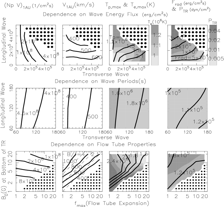
Figure 2: Contours showing dependency of output properties of the solar corona and the solar wind on the input parameters. Panels on the top show dependency on $F_{\rm w,\perp,0}$ and $F_{\rm w,\parallel,0}$, those on the middle show dependency on $\tau_{\perp}$ and $\tau_{\parallel}$, and those on the bottom show dependency on $f_{\rm max}$ and $B_{0}$. Panels on the first column present $(n_{\rm p}v)_{\rm 1AU}(10^{8}{\rm cm^{-2}s^{-1}})$, those on the second column present $v_{\rm 1AU}$(km/s), those on the third column show $T_{\rm p,max}(10^{6}{\rm K})$ (solid lines) and $T_{\rm e,max}(10^{6}{\rm K})$ (filled contours in gray scale), and those on the fourth column show $F_{\rm rad}(10^{5}{\rm erg\;cm^{-2}s^{-1}})$ (solid lines) and $p_{\rm tr}$(dyn cm^-2) (gray contours). Thick dots indicate the parameter sets for which we fail to integrate the energy equations due to too low temperature in the outer region. Dashed lines in panel in the second column on the bottom indicate constant $B_{0}/f_{\rm max}=$4, 2, & 1.

As for parameters, $h_{\perp}$ and $h_{\parallel}$, which control the energy distribution to the protons and electrons from the wave dissipation, we only present the results of the equipartition case adopting $h_{\perp}=h_{\parallel}=0.5$. This must be reasonable for the N-waves, since they work only in the inner corona where the protons and electrons are sufficiently coupled. On the other hand, the approximation might be incorrect for the switch-on shock trains travelling in the outer region ($r>2R_{\odot}$). More energy is injected to the much more massive protons, while the lighter electrons move across the shocks transparently without getting so much energy. Consequently, $h_{\perp}$ might be smaller, though it is inevitable to perform the kinetic simulation to determine $h_{\perp}$ correctly. We have performed the calculation for several models by adopting the extreme value of $h_{\perp}=0$, corresponding to the situation that all the dissipated energy is supplied to the protons. Although these calculations yields larger proton temperature and smaller electron temperature than the equipartition cases, they give quite similar structures of the density and the wind velocity.

Figure 2 illustrates dependency of the output properties on the input parameters in contours. The fiducial values are set as $(F_{\rm w,\parallel,0},F_{\rm w,\perp,0},\tau_{\perp},\tau_{\parallel},f_{\rm max},B_{0})=(3.0\times 10^{5},2.0\times 10^{5},120,120,5,5)$, where $F_{\rm w,\perp,0}$ and $F_{\rm w,\parallel,0}$ in erg cm^-2s^-1, $\tau_{\perp}$ and $\tau_{\parallel}$ in second, and $B_{0}$ in Gauss. Four panels on the top show dependence on $0.5\times 10^{5}\leq F_{\rm w,\perp,0},F_{\rm w,\parallel,0}\leq 5.5\times 10^{5}$, those on the middle show dependence on $60\leq\tau_{\perp},\tau_{\parallel}\leq 180$, and those on the bottom show dependence on $1\leq f_{\rm max}\leq 20$ and $1\leq B_{0}\leq 20$. The first column presents contours of $(n_{\rm p}v)_{\rm 1AU}$, the second column presents those of $v_{\rm 1AU}$, the third column shows those of $T_{\rm p,max}$ and $T_{\rm e,max}$, and the fourth column shows those of $F_{\rm rad}$ and $p_{\rm tr}$. Thick dots in panels on the top and bottom denote models for which we cannot determine the unique coronal structure because we fail to integrate stably the second order derivative of the thermal conduction term due to too low temperature in the outer region.

Four panels on the middle indicate that dependence on the wave periods is quite weak within a range of $60\leq\tau_{\perp},\tau_{\parallel}\leq 180$. In particular almost no dependence results in with respect to $\tau_{\parallel}$ because the most of the energy of the acoustic waves is lost as the downward thermal conduction, being unrelated to $\tau_{\parallel}$. Weak but finite dependences on $\tau_{\perp}$ are consistent with the results obtained by Nakariakov et al.(2000).

Dependency of $(n_{\rm p}v)_{\rm 1AU}$ can be understood in terms of the energy and momentum deposition in the subcritical region. Larger input of $F_{\rm w,\perp,0}$ and $F_{\rm w,\parallel,0}$ directly enhances the energy and momentum inputs to raise $(n_{\rm p}v)_{\rm 1AU}$ (panel in the first column on the top). Smaller $B_{0}$ makes the switch-on shocks dissipate more quickly, since the shock strength, $\alpha_{\rm sh,\perp}$, (eq.(20)), is scaled as $\propto v_{\rm A}^{-3/2}\propto B_{\parallel}^{-3/2}$ (we neglect $v$ in eq.(34)) for fixed $F_{\rm w,\perp}$. As a result, small $B_{0}$ increase the energy and momentum injection in the subcritical region to enhance $(n_{\rm p}v)_{\rm 1AU}$ (panel in the first column on the bottom).

A panel in the second column on the top shows that higher $v_{\rm 1AU}$ is achieved by models with smaller $F_{\rm w,\parallel,0}$. This is because smaller input wave energy flux gives less dense corona and the smaller amount of coronal gas can be effectively accelerated to higher velocity. One of the most important panels is that in the second column on the bottom which illustrates that $v_{\rm 1AU}$ is well correlated with $B_{0}/f_{\rm max}$. $B_{0}/f_{\rm max}$ determines $B_{\parallel}$ in the outer region of $r>r_{1}+\sigma$ where the flow tube expands almost radially (eq.(37)). In models adopting larger $B_{0}/f_{\rm max}$ the acceleration and heating occurs more in the supercritical region than in the subcritical region because $\alpha_{\rm sh,\perp}\propto B_{\parallel}^{-3/2}$, and larger $v_{\rm 1AU}$ yields. Interestingly, the nice correlation between $v_{\rm 1AU}$ and $B_{0}/f_{\rm max}$ is also obtained in recent observation (Hirano et al., 2003), which might be explained by the similar discussion.

Comparison of panels in the third column with those in the first column show that correlation between $T_{\rm e,max}$ and $(n_{\rm p}v)_{\rm 1AU}$ is good. This indicates that $T_{\rm e,max}$ is mainly determined by the energy input in the subcritical region. On the other hand, $T_{\rm p,max}$ is regulated not only by the energy deposition but by the coupling with the electrons; too large input of energy in the subcritical region decreases $T_{\rm p,max}$ since more energy is transfered to the cooler electrons due to the larger density.

Three panels in the fourth column illustrate that $F_{\rm rad}$ and $p_{\rm tr}$ are determined almost solely by $F_{\rm w,\parallel,0}$. The N-waves rapidly dissipate and the heating occurs mainly in the inner corona ($\;\buildrel<\over{\sim}\;1.5R_{\odot}$). The dissipated energy is mostly lost as the downward conduction which finally radiates away in the TR (Hammer, 1982a, b). The radiative loss is determined by the density there according to $\propto\rho^{2}$. Hence, the energy from the N-wave dissipation controls the density at the coronal base and the TR. In other words, larger input of the energy in the inner corona can heat the plasma deeply down to the chromosphere.

Before closing this section, we summarize several important points with respect to the dependency on the input parameters.

1. $F_{\rm rad}$ and $p_{\rm tr}$, or equivalently the density at the coronal base, is mostly determined by $F_{\rm w,\parallel,0}$.

2. The solar wind speed, $v_{\rm 1AU}$, is well correlated with $B_{0}/f_{\rm max}$, whereas it is anticorrelated with $F_{\rm w,\parallel,0}$.

3. Within a range of $60{\rm s}\leq\tau_{\perp},\tau_{\parallel}\leq 180{\rm s}$ the coronal wind structures are affected by $\tau_{\perp}$ and $\tau_{\parallel}$ little.

4. $(n_{\rm p}v)_{\rm 1AU}$, mass flux of the solar wind, depends on all the parameters.

5 Comparison with the Observed High/Low-Speed Solar Wind

5.1 Structure of Corona and Solar Wind

To test reliability of our process in the real solar corona, we study whether our model can account for the difference between the high-speed solar wind from the polar coronal holes and the low-speed solar wind in the equatorial region during the low solar activity phase. The aim of this section is not to show superiority of our process to other heating and acceleration sources but to explore possibilities whether our process can become one of the reliable mechanisms. Recently, two or three dimensional structures have been investigated extensively by numerical simulations (e.g. Roussev et al.2003). However, the self-consistent treatment of the wave propagation is still difficult in such multi-dimensional calculations. Therefore, our one dimensional studies play a complementary role with them.

As we saw in Fig.2, the variation of the wave periods, $60{\rm s}\leq\tau_{\perp},\tau_{\parallel}\leq 180{\rm s}$, affects the results little. Therefore, we look for the model parameters, $F_{\rm w,\perp,0}$, $F_{\rm w,\parallel,0}$, $B_{0}$, and $f_{\rm max}$, for fixed $\tau_{\perp}=\tau_{\parallel}=120$s for simplicity. We summarize below how we determine the input parameters, $F_{\rm w,\perp,0}$, $F_{\rm w,\parallel,0}$, $B_{0}$, and $f_{\rm max}$, which reproduce the data best, based on the arguments in the previous section.

Table 1: Models for the high/low-speed solar wind; $F_{\rm w,\perp,0}$, $F_{\rm w,\parallel,0}$, and $F_{\rm rad}$ in ($10^{5}$erg cm^-2s^-1), $B_{0}$ in Gauss, $(n_{\rm p}v)_{\rm 1AU}$ in $10^{8}$cm^-2s^-1, $v_{\rm 1AU}$ in km/s, $T_{\rm p,max}$ and $T_{\rm e,max}$ in $10^{6}$K, and $p_{\rm tr}$ in $10^{-2}$dyn cm^-2. Note that $B_{0}$ is field strength at the bottom of the TR and $f_{\rm max}$ is also normalized there.

	$F_{\rm w,\perp,0}$	$F_{\rm w,\parallel,0}$	$f_{\rm max}$	$B_{0}$(G)	$(n_{\rm p}v)_{\rm 1AU}$	$v_{\rm 1AU}$	$T_{\rm p,max}$	$T_{\rm e,max}$	$F_{\rm rad}$	$p_{\rm tr}$
High-Speed Wind	2.4	0.36	1	2	3.9	881	2.6	1.2	.42	.38
Low-Speed Wind	4.4	7.2	8	10	4.2	312	1.4	1.4	5.5	5.0

1. The density in the inner corona is regulated almost solely by $F_{\rm w,\parallel,0}$. The observed density in the inner corona ($\;\buildrel<\over{\sim}\;1.2R_{\odot}$) can be explained by $F_{\rm w,\parallel,0}\simeq 3-5\times 10^{4}$erg cm^-2s^-1 for the less dense polar holes and $F_{\rm w,\parallel,0}\simeq 7-9\times 10^{5}$erg cm^-2s^-1 for the denser streamer region (Fig.3).

2. Since the solar wind speed at 1AU is well correlated with $B_{0}/f_{\rm max}$, larger $B_{0}({\rm G})/f_{\rm max}\;\buildrel>\over{\sim}\;2$ is required for the high-speed wind ($v_{\rm 1AU}\;\buildrel>\over{\sim}\;700$km/s) and smaller $B_{0}({\rm G})/f_{\rm max}\simeq 1$ is favorable for the low-speed wind ($v_{\rm 1AU}\;\buildrel<\over{\sim}\;400$km/s).

3. The observed velocity profile in the polar coronal holes shows high outflow speed in the low corona, while the low-speed wind appeared to be accelerated gradually (bottom panel of Fig.3). Jumping to the conclusion, smaller $B_{0}$ is required to reproduce larger $v$ in the inner corona. Since the flow tube does not completely open to $f_{\rm max}$ in the inner corona, smaller $B_{0}$ results in smaller field strength, $B_{\parallel}$, there. Smaller $B_{\parallel}$ anticipates larger $\alpha_{\rm sh,\perp}$ for fixed $F_{\rm w,\perp}$, which let the transverse wave dissipate more in the inner corona. The input of more energy in the subcritical region enhances mass flux, $\rho v$. On the other hand, $\rho$ in the inner corona is independently determined by $F_{\rm w,\parallel,0}$. Consequently, a model adopting smaller $B_{0}$ with identical $F_{\rm w,\perp,0}$, $F_{\rm w,\parallel,0}$, and $B_{0}/f_{\rm max}$ gives larger $v$ in the inner corona.

4. From the above restrictions of (i)-(iii), $F_{\rm w,\parallel,0}$, $B_{0}$, and $f_{\rm max}$ are fixed. The last parameter, $F_{\rm w,\perp,0}$, is tuned to explain the density and the temperature in the intermediate region, $2R_{\odot}\;\buildrel<\over{\sim}\;r\;\buildrel<\over{\sim}\;6R_{\odot}$; too much input of the transverse waves gives too high temperature and also too high density due to too large density scale height, and vice versa.

We tabulate the adopted model parameters and the results of the physical properties of the corona and the solar wind in Tab.1. The structures of the corona and the solar wind in both models are presented in Fig.3 with the observational data.

Figure 3: Comparison of our results of the high-speed solar wind (solid lines) and the low-speed solar wind (dashed lines) with the observed data. In top and middle panels, open symbols are data in the polar coronal holes during the low activity phase and filled symbols are data in the equator or mid-latitude region where the low-speed solar wind is supposed to originates from. Top : Distribution of electron density. Middle : Distribution of proton and electron temperature. Note that proton temperature is higher than electron temperature in both models. bottom : Outflow velocity of the solar wind. Shaded region is observational data in the streamer belt (Sheeley et al., 1997). Data with error bars are outflow speed based on observation of the interplume region in the polar holes (Teriaca et al., 2003)

As shown in Tab.1 we have adopted larger $F_{\rm w,\parallel,0}$ by a factor of 20 in the low-speed wind model than in the high-speed wind model based on the condition (i). This directly leads to larger radiative flux in the low-speed wind model by a factor of 13, which is consistent with observational result that X-ray flux in the quiet-Sun in the low latitude exceed that in the polar coronal holes by more than an order of magnitude (e.g. §1 of Golub and Pasachoff 1999). Accordingly, the transverse waves become relatively important against the slow waves ($F_{\rm w,\perp,0}/F_{\rm w,\parallel,0}\gg 1$) in the high-speed wind, while the longitudinal waves dominant ($F_{\rm w,\perp,0}/F_{\rm w,\parallel,0}<1$) in the dense low-speed wind. Table 1 also shows that the comparable order of the mass flux is realized in the high-speed wind model in spite of smaller input of $F_{\rm w,\perp,0}+F_{\rm w,\parallel,0}$, since smaller $f_{\rm max}$ is adopted and the effect of the adiabatic expansion of the flow tube is reduced.

From the restrictions (ii) and (iii), $B_{0}$ and $f_{\rm max}$ for the high-speed wind model is almost uniquely determined as $(B_{0}({\rm G}),f_{\rm max})=(2,1)$. We choose $(B_{0}({\rm G}),f_{\rm max})=(10,8)$ for the low-speed wind model which shows a little wider acceptable ranges, $6\;\buildrel<\over{\sim}\;B_{0}\;\buildrel<\over{\sim}\;12$ and $5\;\buildrel<\over{\sim}\;f_{\rm max}\;\buildrel<\over{\sim}\;10$. It should be noted that $B_{0}$, the field strength at the bottom of the TR, is smaller than the photospheric value which can be observed, provided that the field lines open out with height in the chromosphere. Although this ambiguity remains, our results of $B_{0}$ are qualitatively consistent with the empirical determination by Sittler & Guhathakurta (1999) giving surface field strength $\simeq 3$G at the pole and $\simeq 15$G at the equator. In a region of $r\;\buildrel>\over{\sim}\;2R_{\odot}$ the field strength ($\propto B_{0}/f_{\rm max}$) in the high-speed wind is lager than that in the low-speed wind, which is opposed to the situation in the low corona, due to the flow tube expansion.

The adopted value, $f_{\rm max}=1$, for the high-speed wind model corresponds to the case of the radial expansion of the flow tube in the corona, which is consistent with the observed radial structure around $1.15-5.5R_{\odot}$ in the polar coronal holes (Woo & Habbal, 1999). However, we would like to point out that our $f_{\rm max}$ is measured from the bottom of the TR, which may be smaller than the observed expansion factor normalized by the photospheric field strength. Our results could become consistent with a reported expansion factor $\simeq 4$ (Goldstein et al., 1996), if the flux divergence of a factor of 4 occurs mainly in the chromosphere.

On the other hand, our analysis has given relatively large $f_{\rm max}$ for the low-speed wind model, which means that the closed structures cover large fraction of the surface. There have been two origins considered with respect to the low-speed wind (see Wang et al.2000 for review). One is the acceleration due to the intermittent break-up of the cusp-shaped closed fields on the equatorial region (e.g. Endeve, Leer, & Holtzer 2003). The other is the acceleration in the open flux tube with large areal expansion in the low- and mid-latitude corona (e.g. Kojima et al.1999), which can be investigated by our modelling. Kojima et al. (1999) detected the low-speed wind with a single magnetic polarity, originating from the open structure region located near the active region. They showed the rapid expansion of the flow tube, being qualitatively consistent with our result, whereas $f_{\rm max}$ cannot be directly compared with the reported expansion factor $\;\buildrel>\over{\sim}\;50$ due to the same reason described above for the high-speed wind model.

The top panel of Fig.3 shows electron density of the high- and low-speed wind model, overlayed with observational data in the polar region (open circles are SUMER/SOHO data by Wilhelm et al. (1998); open stars are UVCS/SOHO data by Teriaca et al. (2003); open triangles and squares are LASCO/SOHO data by Teriaca et al. (2003) and Lamy et al. (1997)) and in the streamer region (filled diamonds and triangles are CDS/SOHO and UVCS/SOHO data at mid-latitude by Parenti et al. (2000); filled pentagons are LASCO/SOHO data at the equator by Hayes, Vourlidas, & Howard (2001)). As for the observations in the polar holes, we present data in the interplume regions when the plume and interplume are distinguished, according as Teriaca et al. (2003) reported a strong evidence in favor of the interplume regions as sources of the high-speed wind. The panel exhibits that our results can explain the trends of the observed electron density well in both models.

The middle panel of Fig.3 compares the results of proton and electron temperature with the observed proton temperature (data with error bars are by Esser et al. (1999); open squares are UVCS/SOHO observation by Antonucci, Dodero, & Giordano (2000)) and electron temperature (open circles are CDS/SOHO observation by Fludra, Del Zanna, & Bromage (1999)) in the polar holes and the observed electron temperature in the mid-latitude streamer (filled diamonds and triangles are CDS,UVCS/SOHO by Parenti et al. (2000)). Please note that the proton temperature is higher than the electron temperature in both models. The results of the proton and electron temperature for the high-speed solar wind show reasonable fits to the data. Our results appeared to be slightly lower than the observed kinetic temperature of the protons by Antonucci et al.(2000; open squares). These data indicate temperature perpendicular to the radial magnetic field. Although our model consider the isotropic distribution of the temperature, it is expected that the heating by the fast-shocks is anisotropic and more effective in the perpendicular direction to the field line (Lee & Wu, 2000). Therefore, our model could give better fitting to the data if taking into account the anisotropic temperature distribution. On the other hand, the temperature for the low-speed wind cannot reproduce the observed high temperature in a region of $1.3R_{\odot}\;\buildrel<\over{\sim}\;r\;\buildrel<\over{\sim}\;1.6R_{\odot}$. It is difficult to reproduce the observation only by adopting larger $\tau_{\perp}$ and $\tau_{\parallel}$ which give slower dissipation. Therefore, we have to say that some other heating mechanisms are required in this region.

The bottom panel of Fig.3 presents outflow velocity of the solar wind. The result of the outflow velocity for the low-speed wind is well inside of the obtained range by the observation of about 65 moving objects in the streamer. On the other hand, our result for the high-speed solar wind is marginally consistent with the data of the lower edge by Teriaca et al. (2003). A cooperation with an extra but less dominant acceleration process would explain the data completely.

5.2 Propagation of Shock Trains

Figure 4 compares the N-waves and the switch-on shock trains in the high- and low-speed wind models. It shows that the dissipation of the N-waves is much more rapid than that of the switch-on shock trains in both models. $\alpha_{\rm sh,\parallel}$ and $F_{\rm w,\parallel}$ is drastic decreasing functions of $r$, while $\alpha_{\rm sh,\perp}$ is more or less constant and $F_{\rm w,\perp}$ decreases gradually. Consequently, dissipation length, $|\mbox{\boldmath${F_{\rm w,\parallel}}$}/\mbox{\boldmath${\nabla\cdot F_{\rm w,\parallel}}$}|$, of the N-waves is very small, $\sim 0.01R_{\odot}$ in $r\;\buildrel<\over{\sim}\;1.5R_{\odot}$. These results indicate that the dissipation of the slow MHD waves is a powerful heating source in the inner corona, which is clearly illustrated in the top panel of Fig.5 comparing heating per unit mass, $Q_{\perp}/\rho$ and $Q_{\parallel}/\rho$. The role of the dissipation of the slow MHD waves is important even in the high-speed wind model, adopting the relatively small $F_{\rm w,\parallel,0}$, to sustain the moderate density at the coronal base through the downward conduction. The top panel of Fig.4 also shows that variations of $\alpha_{\rm sh,\parallel}$ are resemble each other in spite of the large difference of the input energy flux by a factor of 20. This is because the difference of the wave energy flux, $F_{\rm w,\parallel}\sim\rho\alpha_{\rm sh,\parallel}^{2}c_{\rm s}^{3}$, mainly attributes to variation of $\rho$; larger (smaller) input of $F_{\rm w,\parallel,0}$ requires larger (smaller) density through the energy balance between the downward thermal conduction and the radiative loss as discussed so far.

Figure 4: Comparison between the switch-on shock trains and the N-waves in the high-speed wind (solid lines) and low-speed wind (dashed lines). top: Variation of shock amplitudes, $\alpha_{\rm sh,\perp}$ and $\alpha_{\rm sh,\parallel}$, against radius, $r/R_{\odot}$. middle: Variation of wave energy flux, $F_{\rm w,\perp}$ and $F_{\rm w,\parallel}$. bottom: Variation of dissipation length. Total dissipation length, $|\frac{F_{\rm w,\perp}+F_{\rm w,\parallel}}{\mbox{\boldmath${\nabla\cdot(F_{\rm w,\perp}+F_{\rm w,\parallel})}$}}|$, (thick lines) is also displayed with dissipation length for the switch-on shock trains, $|\frac{F_{\rm w,\perp}}{\mbox{\boldmath${\nabla\cdot F_{\rm w,\perp}}$}}|$, and for the N-waves, $|\frac{F_{\rm w,\parallel}}{\mbox{\boldmath${\nabla\cdot F_{\rm w,\parallel}}$}}|$.

Figure 5: Comparison of heating and acceleration in the high-speed wind (Solid lines) and low-speed wind (dashed lines). top: Heating per unit mass from the switch-on shock trains, $Q_{\perp}/\rho$, and from the N-waves, $Q_{\parallel}/\rho$. bottom: Momentum input per unit mass from the switch-on shock trains, $dp_{\rm w,\perp}/(\rho dr)$, is compared with that from the gas pressure, $dp/(\rho dr)$.

The heating from the N-waves is soon dominated by the heating from the switch-on shocks at $\sim 1.1R_{\odot}$ in the high-speed wind model and $1.2R_{\odot}$ in the low-speed wind model. The heating from the switch-on shock trains keeps till a more distant region, which is seen in the top panel of Fig.5. Figure 4 further shows that the dissipation of the switch-on shock trains is more rapid in the low-speed wind model, since the shock amplitude, $\alpha_{\rm sh,\perp}$, is larger in the inner corona (the top panel). This is because $\alpha_{\rm sh,\perp}(\propto\sqrt{\rho^{1/2}B_{\parallel}^{-3}F_{\rm w,\perp}})$ becomes systematically larger in the dense low-speed wind with smaller $B_{0}/f_{\rm max}$.

The dissipation of the switch-on shock trains also contribute directly to the acceleration by the gradient of the wave pressure (eq.(30)). The bottom panel of Fig.5 presents the acceleration per unit mass, $dp_{\rm w,\perp}/\rho dr$, from the switch-on shocks compared with the acceleration from the gas pressure gradient, $dp/\rho dr$. Note that the acceleration from the N-waves is assumed to be zero as it is negligible. The panel indicates that the acceleration by the switch-on shock trains dominates that by the thermal pressure in a region of $3-10R_{\odot}$ in the high-speed wind model, while the gas pressure dominates in the entire region in the low-speed wind model. In summarize, the switch-on shock trains contribute both to the heating and to the acceleration in the high-speed wind, while the low-wind wind is basically driven by the thermal pressure of the coronal plasma which is originally heated by the dissipations of the switch-on shock trains and the N-waves.

The results shown in the bottom panel of Fig.4 allows us to check the validity of the conventional assumption of the constant dissipation length. Total dissipation lengths, $|(F_{\rm w,\perp}+F_{\rm w,\parallel})/(\mbox{\boldmath${\nabla\cdot(F_{\rm w,\perp}+F_{\rm w,\parallel})}$})|$, (thick lines) are at first subject to those of the N-waves in the low corona and eventually to those of the switch-on shock trains in the upper region ($\;\buildrel>\over{\sim}\;1.3R_{\odot}$). Because of the transition, the total dissipation lengths rapidly increase. Even in the outer region they are not constant; they vary $2-6R_{\odot}$ in the high-speed wind model and $0.4-2R_{\odot}$ in the low-speed wind model. Therefore, the assumption of the constant dissipation length is not adequate for our processes.

We would like to discuss the amplitudes, $\alpha_{\rm sh,\perp}$ and $\alpha_{\rm sh,\parallel}$, in connection with the observed non-thermal broadening. Velocity amplitude of the transverse mode in the high-speed wind model becomes $<\delta v_{\perp}>=\frac{1}{\sqrt{3}}\alpha_{\rm sh,\perp}v_{\rm A}\sim 1000({\rm km/s})\times 0.15/\sqrt{3}\simeq 90$(km/s) at its maximum level, where a factor, $\frac{1}{\sqrt{3}}$, comes in for the trains illustrated in Fig.1. On the other hand, the off-limb observation in the polar coronal holes gives non-thermal broadening of $\delta v_{\rm obs}\simeq 30-50$km/s (Banerjee et al., 1998; Doyle, Teriaca, & Banerjee, 1999), which shows that our $<\delta v_{\perp}>$ is not consistent with $\delta v_{\rm obs}$. However, since uncertainties of the projection effects might affect $\delta v_{\rm obs}$, it would be hasty to conclude that our model is ruled out by the observations. Velocity amplitude of the longitudinal mode is as large as $\delta v_{\parallel}=\frac{1}{\sqrt{3}}\alpha_{\rm sh,\parallel}c_{\rm s}\sim 50$km/s at the coronal base in both models, and it decreases to $\delta v_{\parallel}<10$km/s at $r=1.3R_{\odot}$. Nonthermal broadening of 20-40km/s is observed in the solar disk (Erdélyi et al., 1998). Our results are consistent with the observed result except at the coronal base. It is also uncertain whether the discrepancy at the coronal base is real or not, since the same ambiguity comes into the observations of the longitudinal mode.

6 Summary

We have investigated the coronal heating and the acceleration of the high- and low-speed solar wind in the open-field regions by the dissipation of the shock trains. The small reconnection events as well as the surface granulations excite MHD waves not only at the photospheric level but in the corona. Among these waves, the linearly polarized Alfvén waves and acoustic waves steepen through the upward propagation and travel as the switch-on shock trains and N-waves respectively.

Firstly, we derived evolutionary equations for the amplitudes of the shock trains under the WKB approximation by assuming that the dissipation occurs only through the shocks. While the assumptions are supposed to be reasonable for the longitudinal mode, we have to be careful in dealing with the transverse mode because other types of the dissipation mechanisms may be important as well as the WKB approximation becomes marginal in the low corona for the waves with periods of a few minutes. In the future studies, it is required to treat the transverse waves dynamically as taken in Ofman & Davila (1997, 1998); Grappin, Léorat, & Habbal (2002), whereas they consider the wave propagation under the one-fluid approximation.

We determined coronal wind structure consisting of the protons and electrons from the bottom of the TR to 1AU by solving the wave equations simultaneously with the momentum and energy equations. Studies on the dependency on the input parameters give the two important results:

1. $v_{\rm AU}$ has nice correlation with the field strength in the outer region which is proportional to $B_{0}/f_{\rm max}$.

2. The density at the coronal base is almost solely determined by $F_{\rm w,\parallel,0}$.

In the low-speed wind, the acoustic waves play a role to keep the dense corona and smaller $B_{0}/f_{\rm max}\simeq 1$ is required to hold the wind speed slow. On the other hand, in the high-speed wind the transverse waves become relatively important and larger $B_{0}/f_{\rm max}\;\buildrel>\over{\sim}\;2$ is favorable. The early onset of the acceleration in the high-speed wind also requires the weak field strength in the low corona. This accordingly leads to the radial expansion of the flow tube in the corona, though it is not inconsistent with the observed expansion factor $\simeq 4$ in the polar holes if the flux divergence occurs in the chromosphere.

Our model has reproduced the overall trend of the high- and low-speed solar wind except the observed high temperature in the mid-latitude corona connected with the low-speed solar wind. Therefore, our processes could be reliable heating and acceleration mechanisms, whereas contribution from other heating sources are required in the low-speed wind region.

References

- Antonucci, Dodero, & Giordano (2000) Antonucci, E., Dodero, M., A., & Giordano, S. 2000, Sol.Phys., 197, 115
- Banerjee et al. (1998) Banerjee, D., Teriaca, L., Doyle, J. G., & Wilhelm, K. 1998, A&A, 339, 208
- Barnes (1969) Barnes, A. 1969, ApJ, 155, 311
- Belcher (1971) Belcher, J. W. 1971, ApJ, 168, 509
- Boyd & Sanderson (1969) Boyd T. J. M. & Sanderson J. J. 1969, plasma Dynamics (New York: Barnes and Noble)
- Braginskii (1965) Braginskii, S. I. 1965, Rev.Plasma.Phys., 1., 205
- Cranmer, Field, & Kohl (1999) Cranmer, S. R., Field, G. B., & Kohl, J. L. 1999, ApJ, 518, 937
- Doyle, Teriaca, & Banerjee (1999) Doyle, J. G., Teriaca, L., & Banerjee, D. 1999, A&A, 349, 956
- Dusenbery & Hollweg (1981) Dusenbery, P. B. & Hollweg, J. V. 1981, JGR, 86, 153
- Endeve, Leer, & Holtzer (2003) Endeve, E., Leer, E., & Holtzer, T. E. 2003, 589, 1040
- Erdélyi et al. (1998) Erdélyi, R., Doyle, J. G., Perez, M. E., & Wilhelm, K. 1998, A&A, 337, 287
- Esser et al. (1999) Esser, R., Fineschi, S., Dobrzycka, D., Habbal, S. R., Edgar, R. J., Raymond, J. C., & Kohl, J. L. 1999, ApJL, 510, L63
- Fludra, Del Zanna, & Bromage (1999) Fludra, A., Del Zanna, G. & Bromage, B. J. I. 1999, Space Science Review, 87, 185
- Giovanelli (1980) Giovanelli, R. G. 1980, Sol.Phys., 68, 49
- Goldstein et al. (1996) Goldstein, B. E. et al.1996, A&A, 316, 296
- Golub & Pasachoff (1997) Golub, L. & Pasachoff, J. M. 1997, ’The Solar Corona’, Cambridge
- Grappin, Léorat, & Habbal (2002) Grappin, R., Léorat, J., & Habbal, S. R. 2002, JGR, 107, 1380
- Hammer (1982a) Hammer, R. 1982a, ApJ, 259, 767
- Hammer (1982b) Hammer, R. 1982b, ApJ, 259, 779
- Hassler et al. (1990) Hassler, D. M., Rottman, G. J., Shoub, E. C., & Holzer, T. E. 1990, ApJL, 348, L77
- Hayes, Vourlidas, & Howard (2001) Hayes, A. P., Vourlidas, A., & Howard, R. A. 2001, ApJ, 548, 1081
- Heyvaerts & Priest (1983) Heyvaerts, J. & Priest, E. R. 1983, A&A, 117, 220
- Hirano et al. (2003) Hirano, M., Kojima, M., Tokumaru, M., Fujiki, K., Ohmi, T., Yamashita, M, Hakamada, K., and Hayashi, K. 2003, , Eos Trans. AGU, 84(46), Fall Meet. Suppl., Abstract SH21B-0164
- Hollweg (1976) Hollweg, J. V. 1976, JGR, 81, 1649
- Hollweg (1982) Hollweg, J. V. 1982, ApJ, 254, 806 (H82)
- Hollweg (1986) Hollweg, J. V. 1986, JGR, 91, 4111
- Hollweg (1992) Hollweg, J. V. 1992, ApJ, 389, 731
- Hu & Habbal (1999) Hu, Y. Q. & Habbal, S. R. 1999, JGR, 104, 17045
- Hu, Habbal, & Li (1999) Hu, Y. Q., Habbal, S. R., & Li, X. 1999, JGR, 104, 24819
- Jacques (1977) Jacques, S. A. 1977, ApJ, 215, 942
- Katsukawa & Tsuneta (2001) Katsukawa, Y. & Tsuneta, S. 2001, ApJ, 557, 343
- Kojima et al. (1999) Kojima, M., Fujiki, K., Ohmi, T., Tokumaru, M., Yokobe, A., & Hakamada, K. 1999, JGR, 104, 16993
- Kopp & Orrall (1976) Kopp, R. A. & Orall, F. Q. 1976, A&A, 53,363
- Kudoh & Shibata (1999) Kudoh, T. & Shibata, K. 1999, ApJ, 514, 493
- Kulikovskiy & Lyubimov (1965) Kulikovskiy, A. G. & Lyubimov, G. A. 1965, Magnetohydrodynamics, (Addison-Wesley) p.70
- Lamers & Cassinelli (1999) Lamers, H. J. G. L. M. & Cassinelli, J. P. 1999, ’Introduction to Stellar Wind’, Cambridge
- Lamy et al. (1997) Lamy, P., Quemerais, E., Liebaria, A., Bout, M., Howard, R., Schwenn, R., & Simnett, G. 1997 in Fifth SOHO Worshop, The Corona and Solar Wind near Minimum Activity, ed A. Wilson (ESA-SP 404; Noordwijk:ESA), 491
- Landau & Lifshitz (1959) Landau, L. D. & Lifshitz, E. M. 1959, ’Fluid Mechanics’
- Landini & Monsignori-Fossi (1990) Landini, M. & Monsignori-Fossi, B. C. 1990, A&AS, 82, 229
- Lee & Wu (2000) Lee, L. C. & Wu, B. H. 2000, ApJ, 535, 1014
- Marsch, Coertz, & Richter (1982) Marsch, E, Coertz, C. K. & Richter, K. 1982, JGR, 87, 47
- Montgomery (1959) Montgomery, D. 1959, Phys.Rev.Lett., 2, 36
- Nakariakov, Roberts, & Murawski (1997) Nakariakov, V. M., Roberts, B., & Murawski, K. 1997, Sol.Phys., 175, 93
- Nakariakov, Ofman & Arber (2000) Nakariakov, V. M., Ofman, L., & Arber, T. D. 2000, A&A, 353, 741
- MacGregor & Charbonneau (1994) MacGregor, K. B. & Charbonneau, P. 1994, ApJ, 430, 387
- Ofman & Davila (1997) Ofman, L. & Davila, J. M. 1997, ApJ, 476, 357
- Ofman & Davila (1998) Ofman, L. & Davila, J. M. 1998, JGR, 103, 23677
- Ofman, Nakariakov, & DeDorest (1999) Ofman, L., Nakariakov. V. M., & DeDorest, C.E. 1999, ApJ, 514, 441
- Ofman, Nakariakov, & Shegal (2000) Ofman, L., Nakariakov, V. M., & Shegal, N. 2000, ApJ, 533, 1071
- O’Shea, Mulglach, & Fleck (2002) O’Shea, E., Mulglach, K., & Fleck, B. 2002, A&A, 387, 642
- Parenti et al. (2000) Parenti, S., Bromage, B. J. I., Poletto, G., Noci, G., Raymond, J. C., & Bromage, G. E. 2000, A&A, 363, 800
- Press et al. (1992) Press, W. H., Teukolsky, S. A., Vetterling, W. T., & Flannery, B. P. 1992, ’Numerical Recipes in Fortran 77’, Cambridge
- Roberts (2000) Roberts, B. 2000 Sol.Phys., 193, 139
- Roussev et al. (2003) Roussev, I.I., Gombpsi, T. I., Sokolov, I. V., Velli, M., Manchester IV, W., DeZeeuw, D. L., Liewer, P., Tóth, G., & Luhmann, J. 2003, ApJL, 595, L57
- Sakai et al. (2000) Sakai, J.I., Kawata, T., Yoshida, K., Furusawa, K., & Cramer, N. F. 2000, ApJ, 537, 1063
- Sakurai & Granik (1984) Sakurai, T. & Granik, A. 1984, ApJ, 277, 404
- Sandbæk & Leer (1994) Sandbæk, Ø. & Leer, E. 1994, ApJ, 423, 500
- Sheeley et al. (1997) Sheeley, N. R. Jr. et al. 1997, ApJ, 484, 472
- Stein & Schwartz (1972) Stein, R. F. & Schwartz, R. A. 1972, ApJ, 177, 807
- Sittler & Guhathakurta (1999) Sittler, E. C. Jr. & Guhathakurta, M. 1999, ApJ, 523, 812
- Sturrock (1999) Sturrock, P. A. 1999, ApJ, 521, 451
- Suzuki (2002) Suzuki, T. K. 2002, ApJ, 578, 598 (S02)
- Tarbell, Ryutova, & Covington (1999) Tarbell, T., Ryutova, M., & Covington, J. 1999, ApJL, 514, L47
- Teriaca et al. (2003) Teriaca, L., Poletto, G., Romoli, M., & Biesecker, D. A. 2003, ApJ, 588, 566
- Tsuneta (1996) Tsuneta, S. 1996, ApJL, 456, L63
- Wang & Sheeley (1990) Wang, Y.-M. & Sheeley, N. R., Jr. 1990, ApJ, 355, 726
- Wang et al. (2000) Wang, Y.-M., Sheeley, N. R., Socker, D. G., Howard, R. A., Rich, N. B. 2000, JGR, 105, 25133
- Wilhelm et al. (1998) Wilhelm, K., Marcsh, E., Dwivedi, B. N., Hassler, D. M., Lemaire, P., Gabriel, A. H., & Huber, M. C. E. 1998, ApJ, 500, 1023
- Withbroe (1988) Withbroe, G. L. 1988, ApJ, 325, 442
- Woo & Habbal (1999) Woo, R. & Habbal, S. R. 1999, Geo. Res. Lett., 26, 1793