Optimal Moments for Velocity Fields Analysis

We describe a new method of overcoming problems inherent in peculiar velocity surveys by using data compression as a filter with which to separate large–scale, linear flows from small–scale noise that biases the results systematically. We demonstrate the effectiveness of our method using realistic catalogs of galaxy velocities drawn from N–body simulations. Our tests show that a likelihood analysis of simulated catalogs that uses all of the information contained in the peculiar velocities results in a bias in the estimation of the power spectrum shape parameter $\Gamma$ and amplitude $\beta$, and that our method of analysis effectively removes this bias. We expect that this new method will cause peculiar velocity surveys to re–emerge as a useful tool to determine cosmological parameters.

We introduce a new method for the analysis of peculiar velocity surveys $\!{}^{{\bf?},{\bf?}}$ that is a significant improvement over previous methods. In particular, our formalism allows us to separate information about large–scale flows from information about small scales, the latter can then be discarded in the analysis. By applying specific criteria, we are able to retain the maximum information about large scales needed to place the strongest constraints, while removing the bias that small–scale information can introduce into the results.

To analyze the observed line–of–sight velocities we assume that N objects with positions $r_{i}$ and observed line–of–sight velocities $v_{i}$ can be modeled as

$$v_{i}=\vec{v}(\vec{r}_{i})\cdot\hat{r}_{i}+\delta_{i}$$ (1)

where $v(\vec{r}_{i})$ is the linear velocity field and $\delta_{i}$ is the noise which also accounts for the deviations from linear theory. Assume the noise is Gaussian with variance $\sigma_{i}^{2}+\sigma_{*}^{2}$ where $\sigma_{i}$ is the observational error and $\sigma_{*}$ is the contribution from nonlinearity and other things we neglected (see  $\!{}^{{\bf?}}$ for detail analysis). The covariance matrix can be written as

$$R_{ij}=\left\langle{v_{i}\,v_{j}}\right\rangle=R_{ij}^{(v)}+\delta_{ij}\left({\sigma_{i}^{2}+\sigma_{*}^{2}}\right)\qquad{\rm where}\qquad R_{ij}^{(v)}=\left\langle{\vec{v}(\vec{r}_{i})\cdot\hat{r}_{i}\,\,\,\vec{v}(\vec{r}_{j})\cdot\hat{r}_{j}\,}\right\rangle\,.$$ (2)

In linear theory we can express the velocity power spectrum in terms of the density power spectrum and thus rewrite the above as

$$R_{ij}^{(v)}={{H^{2}f^{2}\left({\Omega_{0}}\right)}\over{2\pi^{2}}}\int{P(k)W_{ij}^{2}(k)dk}\,.$$ (3)

The covariance matrix is a convolution of the density power spectrum and the squared tensor window function.

The probability distribution for the line–of–sight peculiar velocities is

$$L\left({v_{1},\cdots,v_{N};P(k)}\right)=\sqrt{\left|{R^{-1}}\right|}\exp\left({{{-v_{i}R_{ij}^{-1}v_{j}}\over 2}}\right)$$ (4)

Alternately, given a set of velocities $\left({v_{1},\cdots,v_{N}}\right)$ we can have $L\left({v_{1},\cdots,v_{N};P(k)}\right)$ to denote the likelihood functional for the power spectrum. Given a power spectrum parameterized by some vector $\Theta=\left({\theta_{1},\cdots,\theta_{s}}\right)$ then $L\left({v_{1},\cdots,v_{N};\Theta}\right)$ is the likelihood functional for the parameter $\Theta.$ The value of the parameter vector that maximizes the likelihood we call $\Theta_{ML}$.

Given a set of true parameter $\Theta_{0}$, we want a maximum likelihood estimator $\langle\Theta_{ML}\rangle=\Theta_{o}$ then $\Theta_{ML}$ will vary over different realizations of $\left({v_{1},\cdots,v_{N}}\right)$. We may characterized our parameters with the Mean $\langle(\theta_{ML})_{i}\rangle$ and the variance $\Delta(\theta_{ML})^{2}_{i}=\langle(\theta_{ML})^{2}_{i}\rangle-\langle(\theta_{ML})_{i}\rangle^{2}$ In the limit of large N: $\langle\Theta_{ML}\rangle=(\Theta_{o})_{i}$ and the variances are minimal.The variances for an unbiased estimators are:

$$\Delta\left({\theta_{ML}}\right)_{i}\geq\left({F_{ii}}\right)^{-1/2}$$ (5)

which is the Cramér–Rao inequality. In the limit of large N this becomes an equality, here we assume that this limit is satisfied. $F_{ii}$ is the trace of the Fisher matrix

$$F_{ij}=\left.{\left\langle{{{\partial^{2}\left({-\ln L}\right)}\over{\partial\theta_{i}\partial\theta_{j}}}}\right\rangle}\right|_{\Theta=\Theta_{0}}$$ (6)

If the velocities are Gaussianly distributed then the maximum likelihood estimator $\Theta_{ML}$ is unbiased. However, actual peculiar velocities contain non–Gaussian contributions, nonlinear contributions will lead to $\Theta_{ML}$ being biased in an unpredictable way. In order to recover an unbiased estimator we utilize data compression methods. We use these methods to filter out unwanted information.

The main purpose of the formalism we presented here and was to allow the removal or filtering of small–scale noise while keeping the large–scale signal. To test the success of the formalism we have created synthetic surveys from simulations with known parameters, specifically, $\Gamma$, the CDM power spectrum shape parameter, and $\beta$, its amplitude. To compare our method with the usual maximum likelihood analysis method, we reemphasize that the optimal moment analysis presented here allows for two semi–independent methods of cleaning up a survey: a) Ordering the moments by their eigenvalues and removing those with the largest eigenvalues b) Removing the noisiest moments. In Fig. 1 we show the comparison between choosing the modes least susceptible to small–scale signal; those that are least susceptible to small–scale signal and are not noisy; and the full analysis (that is, estimating the parameters using all the information). We see that the full analysis fails to recover the “true” parameters by a significant amount ($\approx 4\sigma$ for no errors and $>2\sigma$ for 10% errors). In contrast, the mode analysis recovers the values of the parameters very well, with or without the removal of the noisy moments.

In Fig. 2 we show the value of the estimated parameters as a function of the $\Sigma\lambda^{2}$ where $\lambda$ is the eigenvalue, we see that as the number of modes is increased, we get closer and closer to the “true” value. When we keep more than the number of moments that corresponds to the fulfillment of our criterion (solid vertical lines), the values start diverging systematically from the “true” results. This is due to the fact that small–scale modes that have become nonlinear are introducing a systematic bias. This tendency of the full analysis to systematically overestimate the parameter values can be seen for all values of the parameters.

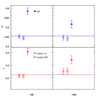
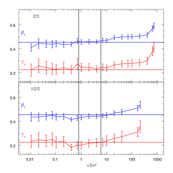
Figure 1: (left panel) A comparison between the mode analysis presented in this paper and the usual full analysis. In the top two panels are the mean values and standard deviations of the mean of $\beta$, the amplitude of the power spectrum. The bottom panels are the results for estimating $\Gamma$, the shape parameter. In the left panels we have the results for the analysis for a survey with no errors whereas the right panels show the results for 10% errors. The solid symbols are the full analysis results and the empty ones are the mode analysis. The triangles are the results without removing the noisy moments, the rectangles are those where we removed the noisiest moments. The horizontal lines are the “true” values of the parameters. Figure 2: (right panel) The mean value of the estimated parameters from 81 catalogs extracted from the simulations as a function of the number of modes we keep. The top panel shows results for survey with no errors, the bottom panel shows the results with distance errors of 10%. As the number of modes kept increases beyond the criteria set, the estimators become systematically biased. The horizontal lines are the “true” values of the parameters.

As was discussed in the text, the reason for the full analysis failure to recover the “true” parameters when the mode analysis succeeds so well can be shown by looking at the window functions themselves. In Fig. 3 we show the normalized window functions $W_{n}(k)$ in arbitrary units vs. $k$, the wave number corresponding to the five lowest eigenvalues and lowest noise (lower left panel). As we move up the panels we see the window functions with larger noise components not removed, whereas when we move to the right we see window functions corresponding to larger eigenvalues. Here the reasons for the particular choices for our criteria become clear. As the eigenvalues or the noise level become large, the window functions generally probe more small–scale and less of large–scale modes. Since we are primarily interested in large–scale information, discarding the noisy, high $\lambda$ modes allows us to remove small–scale signal that might, and generally does, interfere with with our analysis.

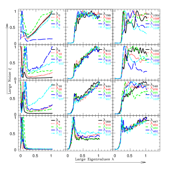
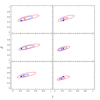
Figure 3: (left panel) The window functions $W_{n}(k)$ in arbitrary units, from top to bottom corresponding to noise in the ranges of $0.98<\xi$, $0.95<\xi<0.98$, $0.9<\xi<0.95$ and $\xi<0.9$ respectively, and across from left low, medium and high eigenvalues $\lambda$ respectively. We can clearly see that the low eigenvalue low noise window functions (lower left panel) probe large scale (small $k$), whereas higher noise, larger eigenvalue window functions (up and to the right) correspond to smaller scales probes. Figure 4: (right panel) The maximum likelihood contours from six typical mock catalogs. The contours are the 68% and 94% likelihood lines. In most cases the uncertainties in the estimated values of the parameters $\Gamma$ and $\beta$ are of comparable sizes to the monte carlo errorbars presented in figures 1

In Fig. 4 we show the contours that contain 68% and 94% of the total likelihood for six typical catalogs. The diamond shows the maximum likelihood results, whereas the asterisk in each panel shows the “true” values of the parameters. These contours allow us to estimate the uncertainty in the maximum likelihood values obtained from the analysis of a single catalog, as is the case when analyzing observational data. From the figures it is clear that the uncertainties obtained in this way are comparable to those we get from the Monte–Carlo simulations. In general, when we try to test the reliability of results from an observational data set, we apply our formalism to mock catalogs extracted from N–body simulations as was done here. This compatibility between the uncertainties obtained in two different ways gives us confidence that using the likelihood contours will give us an accurate assessment of the uncertainties of our maximum likelihood values when we apply our method to real catalogs.

We have described the power and elegance of a new statistic that was designed and formulated in order to address a crisis in the analysis of proper distance cosmological surveys. We have shown that our formalism mostly overcomes the problems with the traditional analysis of the data. Whereas the full maximum likelihood analysis tends to systematically overestimate the values of the parameters that describe the power distribution on large scale, our mode analysis makes very accurate estimates of these parameters.

As was shown in our recent publications $\!{}^{{\bf?},{\bf?}}$, the formalism is highly adaptive and versatile. It can be applied surveys with any geometry and density, and since it retains maximum information should be particularly useful for sparse data such as that obtained in cluster peculiar velocity surveys. Overall, we consider this method to be a significant improvement over previous methods used for the analysis of peculiar velocity data.

References

References

- [1] Watkins, R., Feldman, H. A., Chambers, W., Gorman, P. & Melott, A., 2002, ApJ 564 534–541
- [2] Feldman, H. A., Watkins, R., Melott, A. & Chambers, W., 2003, astro–ph/0304316
- [3] Feldman, H. A. & Watkins, R., 1994, ApJ Lett. 430 L17–20.