Infrared Spectroscopic Study of 8 Galactic Globular Clusters

Abstract

We have obtained medium-resolution infrared $K$ band spectra of 44 giants in seven heavily reddened clusters in the Galactic bulge, as well as 12 giants in $\omega$ Centauri. We measure the equivalent widths of the Na doublet, the Ca triplet, and the CO band head, and then apply the new technique of Frogel et al.to determine the metallicity of each star. Averaging these values, we estimate the metallicity for each cluster, and compare our new [Fe/H] values with previous determinations from the literature. Our estimates for each cluster are: NGC 6256 ($-1.35$), NGC 6539 ($-0.79$), HP 1 ($-1.30$), Liller 1 ($-0.36$), Palomar 6 ($-0.52$), Terzan 2 ($-0.87$), and Terzan 4 ($-1.62$). We briefly discuss differences between the various [Fe/H] scales on which it was possible to base our calibration, which is found to be the largest uncertainty in using this technique to determine metallicities.

1. Introduction

The globular clusters of the Milky Way consist of two distinctly separated groups, each with approximately Gaussian metallicity ([Fe/H]) distributions. This bimodality was first quantified by Freeman & Norris (1981), Zinn (1985), and Armandroff & Zinn (1988). The mean [Fe/H] values for the two groups are approximately $-0.5$ and $-1.6$. As detailed by these authors and many others since then, the bimodality is not confined just to the distribution over [Fe/H]. The two groups have quite distinct spatial distributions and kinematical properties as well. The metal-poor group contains classical, population II halo objects in terms of their location and space motions, in addition to their low metallicities. Clusters in the metal-rich group, on the other hand, are mostly confined to the same volume of space as the Galactic bulge. Of the 33 clusters with [Fe/H] $\geq-0.7$ (data from Harris (1996) as updated in 2003 February), three-quarters of them lie within 20° of the Galactic center, and half lie within 10° of the center. Not surprisingly, these clusters are also heavily reddened; the average $E(B-V)$ of the sample that lies within 10° of the Center is 1.41, which is equivalent to an average visual extinction ($A_{V}$) of 4.4 mag. The problems associated with optical studies of these clusters are further compounded by the fact that many of them lie in very crowded fields and are not themselves of high surface brightness or concentration.

An obvious question to ask concerning the metal-rich globular clusters is whether they are in some way physically associated with the bulge, sharing a common origin and evolution, as has been argued by many authors (e.g. Minniti, 1995b; Côté, 1999); or is the similarity in spatial distribution of the clusters and bulge stars merely coincidental and due simply to the influence of the same gravitational potential. If the former is the case, then knowledge of these metal-rich clusters would be particularly relevant in enhancing our understanding of the formation and evolution of the bulge itself. Accurate abundance determinations for these clusters would be of particular importance. However, because of the difficulties associated with observing these clusters in the optical, spectroscopic abundances based on observations of individual stars are available for only a small fraction of those that lie closer than 15° from the Galactic center. The situation is somewhat better in terms of deriving physical parameters from optical color-magnitude diagrams (CMDs); of particular note is the program being carried out by Ortolani and his collaborators (Ortolani, Bica & Barbuy, 1997a, and references therein).

In working toward this goal of learning more about these heavily reddened bulge clusters, we have recently developed a new method for the determination of [Fe/H] for globular clusters based on the measurement of absorption features due to Ca, Na, and CO in the $K$ band spectra of a few of the brightest giants in each cluster (Frogel et al., 2001, hereafter Paper I). The practical advantages of the near-IR technique we have developed are several and important. The necessary spectroscopic observations are at a resolution of only $\approx 1500$ and need only be obtained for the brightest half-dozen or so giants in a cluster. Knowledge of cluster reddening or distance is not needed, although if dereddened colors and absolute $K$ band magnitudes are known, the accuracy of the resulting [Fe/H] value is further improved. Furthermore, because of the close coupling between [Fe/H] and the location and morphology of a cluster’s red giant branch (RGB), our technique is largely insensitive to the choice of stars so long as they are on the upper 3 or 4 mag ($K$ band) of the RGB. This advantage was also demonstrated in our study of giants in the field of the Galactic bulge (Ramírez et al., 2000). In the $K$ band the giants near the top of a cluster’s RGB are very bright in contrast to their relative faintness in $V$, which is due to severe molecular blanketing. And, finally, a consequence of the previous fact is that the effects of crowding and confusion with field stars are significantly reduced.

2. Selection of Clusters, Observations, Data Reduction

For this paper we chose seven poorly studied globular clusters located in or near the Galactic bulge, which are believed to have [Fe/H] $\geq-1.0$ and/or are heavily reddened. For five of these clusters, our work is the first detailed spectroscopic study of individual cluster stars. Table 1 summarizes some of the properties of these clusters.

Table 1Clusters observed & some previous metallicity determinations

Cluster	l	b	$E(B-V)$	[Fe/H]ZW84	[m/H]W85	[Fe/H]AZ88	[$Z/Z_{\odot}$]B98	[Fe/H]H03
NGC 6256	$-12.2$	3.3	1.03	…	$-1.56$	…	$-1.01$	$-0.70$
NGC 6539	20.8	6.8	0.97	$-0.66$	$-1.05$	…	…	$-0.66$
HP 1	$-2.6$	2.1	0.74	…	$-1.68$	$-0.56$	$-1.09$	$-1.55$
Liller 1	$-5.2$	$-0.2$	3.06	$-0.21$	$-0.29$	$+0.20$	$+0.08$	$+0.22$
Palomar 6	2.1	1.8	1.46	$-0.74$	$+0.22$	…	$-0.09$	$-1.09$
Terzan 2	$-3.7$	2.3	1.57	$-0.47$	$-0.54$	$-0.25$	$-0.26$	$-0.40$
Terzan 4	$-4.0$	1.3	2.35	$-0.21$	$-0.29$	$-0.94$	$-0.61$	$-1.60$
$\Delta$[Fe/H]				$0.37\pm 0.62$	$0.23\pm 0.62$	$0.64\pm 0.08$	$0.50\pm 0.28$	$0.14\pm 0.45$

Most previous estimates of [Fe/H] values for these seven clusters are from the characteristics of their optical or near-IR CMDs, or from integrated spectroscopy. Integrated spectroscopy of globular clusters that are in the very crowded Galactic bulge region, especially optical spectroscopy, will almost always tend to overestimate [Fe/H] because of contamination from metal-rich bulge giants (see the discussion in Section 6).

Our spectroscopic data were obtained on the Blanco 4 m telescope at the Cerro Tololo Inter-American Observatory (CTIO) with either CTIO’s near-IR spectrometer (IRS; R=1650, DePoy et al., 1990) or with the Ohio State InfraRed Imager/Spectrograph (OSIRIS; R=1380, DePoy et al., 1993). Spectral coverage was generally between 2.17 and $2.34\mu$m. Most of our observations were made on the same nights as those for the calibration clusters (Paper I); details of the observations and data reduction for these seven clusters are identical to those described in Paper I, and so will be only briefly described here.

Each spectrum begins as a set of $\sim 10$ individual spectra taken by stepping the star along the slit to eliminate the effects of uneven slit illumination, bad pixels, and fringing. The slit is several arc minutes long, which permits simultaneous star and sky measurements. The array response signature is first removed by dividing each of the individual frames by a dome flat field. The sky frame for each star is formed by median-combining the individual frames in each set, thus removing all traces of the star itself, and then subtracting it from each spectral frame. Each spectra in a set is then extracted using the IRAF apall routine. The final spectrum for a star is the average of the extracted individual spectra.

The wavelength calibration for each star is determined by fitting to approximately 12 atmospheric OH lines (Oliva & Origlia, 1992) visible on a sky spectrum, where the sky spectrum is extracted from the sky frame using the program star as an extraction template. We fit the observed wavelengths to the laboratory ones with a second order Legendre polynomial.

To remove telluric absorption features from each final stellar spectrum, we divide them by a normalized standard star spectrum to correct for telluric absorption features and then multiply by a 10,000 K blackbody spectrum to restore the over all shape of the spectrum. These standard stars are of early A spectral type or hotter, with no significant spectral features in the observed wavelength regime, except for Brackett $\gamma$ at 2.16 $\mu$m. They are observed as close in time and air mass as practical to the observations of each cluster star.

The technique we use to measure the equivalent widths (EWs) of the spectral features – EW(Na), EW(Ca), and EW(CO) – is described in Paper I. Table 2 gives the continuum and line regions over which we integrate. Note that EW(CO) does not include any contribution from the ¹³CO band head. EW(Ca) and EW(Na) have continuum regions on either side of the line absorption region and thus are independent of changes in the spectral slope due to reddening. There is no viable continuum region to the red of the CO band head, so instead we extrapolate a linear fit to the continuum blueward of the feature and integrate the depth of the absorption under this extrapolated continuum. Although the slope of the fitted continuum will change with reddening, the integrated absorption equivalent width under the continuum should stay constant.

Table 2Equivalent Width Measurement Intervals

Feature	Wavelengths (µm)
Na I feature	2.2040 - 2.2107
Na I continuum	2.1910 - 2.1966
Na I continuum	2.2125 - 2.2170
Ca I feature	2.2577 - 2.2692
Ca I continuum	2.2450 - 2.2560
Ca I continuum	2.2700 - 2.2720
12CO(2,0) band	2.2915 - 2.3025
12CO(2,0) continuum	2.1900 - 2.2010
12CO(2,0) continuum	2.2110 - 2.2220
12CO(2,0) continuum	2.2330 - 2.2600
12CO(2,0) continuum	2.2680 - 2.2800
12CO(2,0) continuum	2.2860 - 2.2910

Table 3 gives the observed spectroscopic indices for each star, and when available, colors and magnitudes. The photometry is from Frogel, Kuchinski & Tiede (1995) for Liller 1, Kuchinski et al. (1995) for Terzan 2, and Frogel & Sarajedini (1998, private communication) for Terzan 4. Measurement uncertainties for the spectroscopic indices are typically 0.3, 0.4, and 0.6 Å for Na, Ca, and CO, respectively, calculated from the errors associated with fitting the continuum. However, an analysis of duplicate measurements taken over several years and with different instruments yields slightly higher values (see Table 3 of Paper I).

Table 3Near-IR Spectral Indices, Colors, and Luminosities

				EW (Å)
Cluster	Star	$M_{K0}$	$(J-K)_{0}$	Na	Ca	CO	[Fe/H]
NGC 6256	51	…	…	0.60	0.71	6.52	-1.37
NGC 6256	93	…	…	0.67	0.85	5.51	-1.37
NGC 6256	95	…	…	0.79	0.37	3.37	-1.41
NGC 6256	162	…	…	1.01	0.40	4.20	-1.31
NGC 6256	B	…	…	0.71	0.46	8.05	-1.29
NGC 6539	1	…	…	1.99	2.84	16.83	-0.67
NGC 6539	2	…	…	1.88	2.35	15.27	-0.76
NGC 6539	3	…	…	1.85	2.71	16.45	-0.72
NGC 6539	4	…	…	1.31	1.55	12.34	-0.99
HP 1	46	…	…	0.63	0.93	5.73	-1.38
HP 1	57	…	…	4.80	4.30	22.69	-0.25
HP 1	191	…	…	4.63	4.01	21.35	-0.29
HP 1	435	…	…	0.62	1.21	11.92	-1.22
HP 1	A	…	…	4.03	2.98	21.14	-0.42
HP 1	B	…	…	2.83	3.22	18.50	-0.48
Liller 1	6	-6.50	1.17	3.57	4.63	21.43	-0.16
Liller 1	7	-6.45	1.13	2.35	5.34	14.53	-0.59
Liller 1	157	-6.80	0.93	4.22	5.62	21.23	-0.23
Liller 1	158	-6.62	1.13	3.15	4.32	20.93	-0.32
Liller 1	160	-6.50	1.27	2.22	2.04	12.28	-0.66
Liller 1	162	-6.05	1.16	2.46	3.27	18.00	-0.45
Liller 1	166	-5.47	0.95	3.07	3.16	11.58	-0.56
Liller 1	299	-6.73	1.38	3.93	5.34	21.88	0.07
Palomar 6	1	…	…	3.81	4.71	21.42	-0.16
Palomar 6	2	…	…	2.65	2.94	18.01	-0.54
Palomar 6	3	…	…	0.97	-1.14	12.64	-1.03
Palomar 6	4	…	…	1.11	-1.94	17.02	-0.85
Palomar 6	5	…	…	4.64	3.04	22.40	-0.43
Palomar 6	11	…	…	4.55	4.75	18.54	-0.16
Palomar 6	14	…	…	2.78	1.77	17.33	-0.63
Terzan 2	1	-5.82	0.82	1.37	2.18	12.45	-1.07
Terzan 2	2	-5.78	0.95	1.02	2.39	17.15	-0.83
Terzan 2	3	-5.73	0.99	4.86	4.03	22.39	0.27
Terzan 2	4	-5.72	0.85	1.93	2.36	18.16	-0.74
Terzan 2	5	-5.46	0.97	0.83	2.85	16.67	-0.79
Terzan 2	7	-5.36	0.88	1.32	3.23	16.58	-0.76
Terzan 2	8	-5.33	0.87	0.82	1.83	11.67	-1.04
Terzan 4	185	-6.44	0.74	0.97	0.91	6.28	-1.49
Terzan 4	333	-6.25	0.84	1.16	-0.15	7.67	-1.33
Terzan 4	399	-6.69	0.73	-0.07	1.96	-0.78	-1.90
Terzan 4	424	-6.11	0.69	-0.01	2.02	1.45	-1.77
Terzan 4	453	-6.61	0.85	0.01	0.85	8.70	-1.57
Terzan 4	461	-5.92	0.70	-0.33	0.31	3.18	-1.80
Terzan 4	474	-6.22	0.78	0.35	0.89	9.20	-1.48

Column 2 of Table 3 lists the stars observed in each cluster. The identifications for Liller 1 are from Frogel, Kuchinski & Tiede (1995), and the identifications for Terzan 2 are from Kuchinski et al. (1995). The numbering schemes for the remaining clusters are completely arbitrary. We therefore provide finding charts for NGC 6256 in Figure 1, NGC 6539 in Figure 2, HP 1 in Figure 3, Palomar 6 in Figure 4, and Terzan 4 in Figure 5. The last column of Table 3 lists the metallicity derived for each star as discussed in the next section.

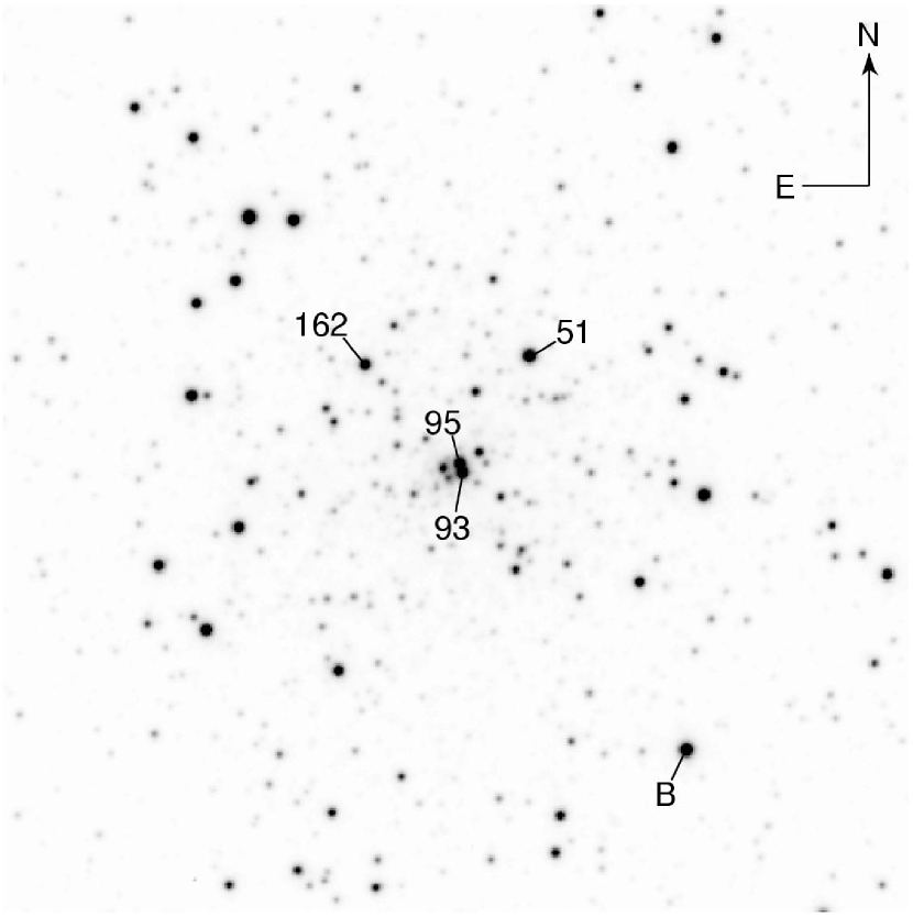
Figure 1.— The $2^{\prime}\times 2^{\prime}$ $I$ band finder chart for the stars observed in NGC 6256.

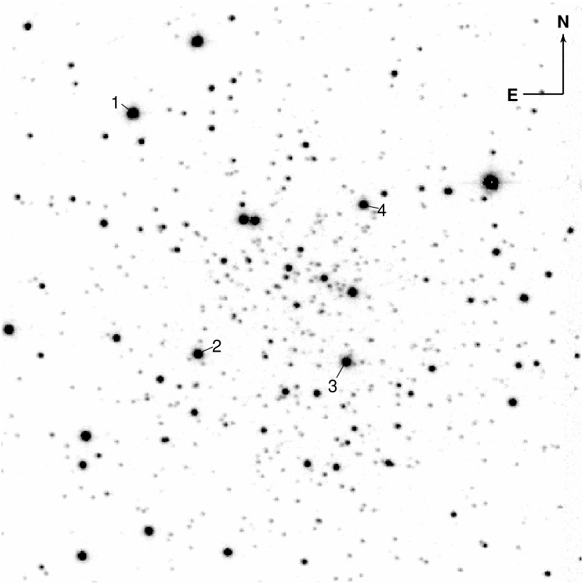
Figure 2.— The $2^{\prime}\times 2^{\prime}$ $K$ band finder chart for the stars observed in NGC 6539.

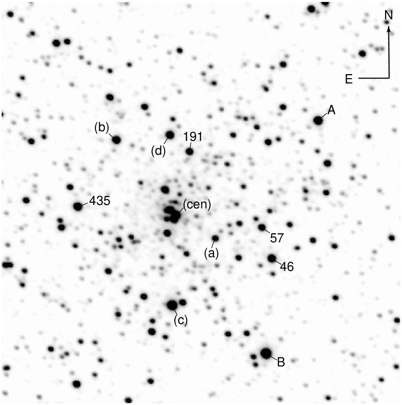
Figure 3.— The $1.5^{\prime}\times 1.5^{\prime}$ $I$ band finder chart for the stars observed in HP 1. The letters in parentheses mark stars observed spectroscopically by Minniti (1995a)(a,b,c,d,cen).

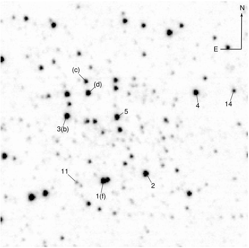
Figure 4.— The $2^{\prime}\times 2^{\prime}$ $K$ band finder chart for the stars observed in Palomar 6. The letters in parentheses mark stars observed spectroscopically by Lee & Carney (2002) (a-g), and by Minniti (1995a)(b,c,d,f).

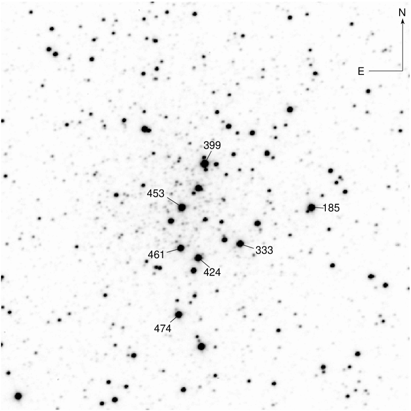
Figure 5.— The $1^{\prime}\times 1^{\prime}$ $I$ band finder chart for the stars observed in Terzan 4.

For clusters without calibrated near-IR photometry (either our own or that of others), we constructed instrumental color-magnitude diagrams from new $JK$ images taken under non-photometric conditions, and chose the brightest stars near the cluster centers with colors and magnitudes consistent with membership. For clusters that physically lie within particularly crowded bulge fields, this may still not preclude the inclusion of non-members, since bulge giants will suffer from the same degree of reddening and will have colors and magnitudes similar to those of giants in the clusters, especially the metal rich clusters. Table 4 gives the cluster mean values for the indices and photometric parameters, along with the star-to-star intra cluster dispersions. The two entries for HP 1 will be explained later.

Table 4Cluster Mean Values and Dispersions for Observed Parameters

		EW(Na)		EW(Ca)		EW(CO)		$M_{K0}$		$(J-K)_{0}$
Cluster	$N_{stars}$	mean	$\sigma$	mean	$\sigma$	mean	$\sigma$	mean	$\sigma$	mean	$\sigma$
NGC 6256	5	0.76	0.16	0.56	0.21	5.53	1.86	…	…	…	…
NGC 6539	4	1.76	0.30	2.36	0.58	15.22	2.03	…	…	…	…
HP 1 weak	2	0.63	0.01	1.07	0.20	8.83	4.38	…	…	…	…
HP 1 strong	4	4.07	0.89	3.63	0.63	20.92	1.75	…	…	…	…
Liller 1	8	3.12	0.75	4.21	1.28	17.73	4.33	-6.39	0.44	1.14	0.15
Palomar 6	5	3.15	1.48	2.11	2.50	18.66	2.17	…	…	…	…
Terzan 2	7	1.74	1.43	2.70	0.74	16.44	3.60	-5.60	0.21	0.90	0.07
Terzan 4	7	0.30	0.56	0.97	0.80	5.10	3.86	-6.32	0.27	0.76	0.06

Note. — Pal 6 Excludes the 2 known non-members.

Figure 6 illustrates, for each cluster except HP 1, the average of the individual stellar spectra. Here we have indicated the three features measured, the Na i doublet, the Ca i triplet, and the first band head of CO. For reference, we have also marked a strong Fe i line and the second band head of CO.

Figure 6.— Average of the individual stellar spectra for each cluster observed, except for HP 1 (see Fig. 7). The positions of the Na i doublet, a strong Fe i line, the Ca i triplet, and the first two band heads of CO are indicated. Only the ¹²CO(2,0) band is used for determining EW(CO). Note the relative absence of spectral features in NGC 6256 and Terzan 4. The high S/N of the spectra is also evident.

Figure 7 shows the individual stellar spectra for all stars observed in HP 1. Note that the first two of the HP 1 stars have significantly weaker absorption features than the other four stars. For comparison, we also show the spectrum of a low-latitude Galactic bulge star with similar colors and indices as the “strong” HP 1 stars from Ramírez et al. (2000).

Figure 7.— $K$ band spectra of the six stars observed in HP 1, and the spectrum of an inner galactic bulge star with similar colors and luminosity for comparison (Ramírez et al., 2000). The first two stars, 46 and 435, clearly have much weaker features than the other four stars in HP 1. These first two stars are therefore referred to as the “weak” group, while the latter four are referred to as the “strong” group.

3. Derivation of Cluster Metallicities

Paper I investigated techniques to use spectroscopic features measured in medium-resolution infrared spectra to measure globular cluster metallicities. The three strongest features in the $K$ band spectrum are the Na i doublet, the Ca i triplet, and the first band head of CO.

It is well known that each of these features has its own problems as a metallicity indicator. [Na/Fe] can show significant star-to-star variations within a single cluster; Sneden, Pilachowski, & Kraft (2000) have measured $\sigma$[Na/Fe]$\simeq 0.25$ dex in M15 and M92. Calcium is an $\alpha$-element, and thus suffers from $\alpha$-enhancement, which varies from cluster to cluster and systematically with overall abundance (Carney, 1996). The first-overtone CO band heads in the $K$ band saturate at high metallicities, making them less sensitive to carbon abundance and more dependent on the microturbulent velocity.

While each of these features has its own shortcomings as a metallicity indicator, taken together and averaged over several stars in a cluster, we have demonstrated that they nonetheless provide a precise metallicity determination (Paper I). Including stellar luminosities and colors, which help constrain the stellar temperature and gravity, improves the technique even further.

Taking advantage of these facts, in Paper I we derived four equations with which one can calculate [Fe/H] for globular cluster giants. These equations use either linear or quadratic combinations of the measured equivalent widths of Na, Ca, and CO, and, optionally, the infrared color and luminosity (Table 10 of Paper I). These equations are applied to each observed star in a cluster to predict [Fe/H] for that star. The unweighted average of these values is then the [Fe/H] assigned to the cluster. Solutions LL3 and QQ3, linear and quadratic, respectively, use only the three spectroscopic indices; therefore, they are independent of reddening and distance to the clusters. Solutions LLA9 and QQA9 also incorporate the $(J-K)_{0}$ colors and $M_{K}$ magnitudes. Thus, while [Fe/H] estimates from LLA9 and QQA9 use more information and can be more precise, they are also affected by uncertainties in the reddening and distance estimates. Table 5 lists the coefficients for the four equations; it is an abbreviated version of Table 10 from Paper I. The last line of Table 5 is our estimate of the typical uncertainty of the metallicity derived from each solution. It is based on the scatter of the individual stellar determinations in each of the calibrating clusters with six to nine stars observed per cluster. It does not include any uncertainties introduced by the observations of clusters to which the calibration is being applied, $e.g.$ errors in calculating the distance modulus or reddening for the solutions that employ colors and absolute magnitudes. Nor does it include the absolute uncertainty of the metallicity scale, which is discussed in section 3.2.

Table 5The Linear and Quadratic Solutions for [Fe/H]

	LL3		LLA9		QQ3		QQA9
variable	coef	$\sigma$	coef	$\sigma$	coef	$\sigma$	coef	$\sigma$
const	-1.663	0.057	-1.451	0.18	-1.811	0.074	1.097	1.16
EW(Na)	0.182	0.029	0.202	0.036	0.389	0.065	0.130	0.091
EW(Na)2	…	…	…	…	-0.047	0.013	0.016	0.020
EW(Ca)	0.057	0.025	0.025	0.026	-0.030	0.051	0.058	0.056
EW(Ca)2	…	…	…	…	0.024	0.012	-0.004	0.014
EW(CO)	0.027	0.005	0.026	0.005	0.043	0.013	0.028	0.016
EW(CO)2	…	…	…	…	-0.001	0.000	0.000	0.001
$(J-K)_{0}$	…	…	0.749	0.23	…	…	5.240	1.84
$(J-K)_{0}^{2}$	…	…	…	…	…	…	-2.313	0.93
$M_{K}$	…	…	0.151	0.033	…	…	1.812	0.40
$M_{K}^{2}$	…	…	…	…	…	…	0.147	0.034
$\sigma$ (est)	0.11		0.07		0.09		0.06

Table 6 lists the average abundances calculated for each cluster from the four solutions in Table 5. The second column indicates the number of stars observed in each cluster. The sigma is the star-to-star scatter for each cluster. While there are no significant differences in the means between the [Fe/H] values from any of the solutions, based on the estimated error and the observed star to star scatter for each solution, we choose a “best” metallicity for each cluster and give the results in Table 8. These are computed on a cluster-by-cluster basis, as described in section 4. The metallicity of each star, as used in the calculation of the “best” value for each cluster, is also listed in the last column of Table 3.

Table 6Cluster Abundances

		LL3		LLA9		QQ3		QQA9
Cluster	$N_{stars}$	[Fe/H]	$\sigma$	[Fe/H]	$\sigma$	[Fe/H]	$\sigma$	[Fe/H]	$\sigma$
NGC 6256	5	-1.34	0.04	…	…	-1.35	0.05	…	…
NGC 6539	4	-0.80	0.14	…	…	-0.79	0.14	…	…
HP 1 weak	2	-1.25	0.13	…	…	-1.30	0.11	…	…
HP 1 strong	4	-0.15	0.24	…	…	-0.36	0.11	…	…
Liller 1	8	-0.38	0.29	-0.36	0.25	-0.31	0.28	-0.30	0.29
Palomar 6	5	-0.47	0.44	…	…	-0.52	0.25	…	…
Terzan 2	7	-0.75	0.38	-0.77	0.40	-0.83	0.27	-0.71	0.45
Terzan 4	7	-1.42	0.15	-1.62	0.21	-1.53	0.28	-1.60	0.23

Note. — Pal 6 Excludes the 2 known non-members.

3.1. How many Stars are Enough?

One may ask how many stars are required to obtain a reliable measure of the metallicity of a cluster. In the clusters presented here we have tried to obtain spectra of more than 5 stars in each; however, because of time or weather constraints, this may not always have been possible; for example, in NGC 6539 we only have spectra of four stars. In such cases, where only a few stars have been measured, it becomes desirable to know with what accuracy and precision one can determine the cluster metallicity. Is it possible, for example, to get away with only measuring one or two or three stars with our technique?

One important consideration is the potential contamination from superposed field stars. With a large sample of spectra it is possible to effectively reject a few non-members if their metallicities are sufficiently different from that of the cluster. However, with a reduced sample size it becomes impossible to distinguish between members and nonmembers.

A way to test the robustness of our metallicity determinations against small sample sizes is to run Monte Carlo simulations on some of the clusters that have larger samples, and therefore relatively well-determined metallicities. To simulate the results of only measuring $N$ stars in a cluster, we randomly select stars from the observed sample and average their metallicities to determine that of the cluster. By repeating this process $100,000$ times, we accumulate the distribution of errors, and can therefore estimate the accuracy and precision with which one can determine the cluster metallicity using only a sample of $N$ stars.

Two illustrative examples are the spectra of the clusters Terzan 2 and Terzan 4. In Terzan 4 we measured seven stars that have a reasonably narrow distribution of metallicities; therefore, picking even a few stars gives a reasonable result for the cluster. On average, only measuring one star will give the correct answer, but the distribution of results has a sigma of 0.19 dex. Averaging the results from two stars, the width of the distribution is reduced to 0.12 dex, and with three stars it drops to 0.09 dex.

Terzan 2 also has a relatively narrow distribution of metallicities, except that, of the seven measured stars, one appears to be a field star with a much higher metallicity. In our analysis in Sec 4.6 we recognize this fact, and disregard the outlier when determining our “best” value for the cluster. However, with a smaller sample, it would be much more difficult to recognize contaminants. This is shown in the simulations, where on average, the deviation from the “best” value is 0.16 dex. Only measuring one star yields a distribution with a sigma of 0.42 dex; the mean of two stars give a sigma of 0.27 dex, three a width of 0.20 dex, etc.

Thus, the appropriate number of spectra for an accurate measure of the cluster metallicity (where accurate means to within the accuracy of the technique) appears to be most dependant on the severity of the non-member contamination. If one expects no contaminants, e.g. an isolated cluster, three stars are sufficient to reduce the stochastic noise inherent when using spectra of the signal-to-noise ratio (S/N) presented here (consistent with what was found in Paper I). However, in more polluted regions, such as the Galactic disk or bulge, more stars are required to be able to effectively reject non-members. Furthermore, the number of stars required increases as the difference between the cluster metallicity and the contaminating population decreases.

3.2. The Metallicity Scale

The calibration of the current technique used the metallicities listed in the 1999 version of the Harris catalog (Harris, 1996) of Galactic globular clusters, which is a continually changing average of parameters taken from literature. Thus, while Harris started out on the Zinn & West (1984) scale, the catalog has been evolving as more and more values from high-resolution spectroscopy are incorporated. However there exist significant discrepancies observed between metallicities obtained with various techniques, and on the absolute calibration of the metallicity scale itself.

The Zinn & West (1984, hereafter ZW84) metallicity scale was one of the first such metallicity scales. Calibrated primarily from the spectroscopy of Cohen (see Cohen, 1983, and references therein), it used photometric indices measured from cluster integrated light, and was applied to a total of 121 clusters. This scale has been updated by Rutledge, Hesser & Stetson (1997) using low-resolution spectroscopic measurements of the red Ca II triplet in individual giants.

The Carretta & Gratton (1997, hereafter CG97) [Fe/H] scale is based on a uniform analysis of high-resolution spectra of more than 160 bright red giants in 24 globular clusters. Figure 5 of CG97 shows a comparison between their system and that of ZW84: a nonlinear relation where the ZW84 values are $\sim 0.1$ dex too high at the metal-rich end ([Fe/H]$>-1$), and $\sim 0.2$ dex too low for clusters of intermediate metallicity ($-2<$[Fe/H]$<-1$).

The recent work by Kraft & Ivans (2003, hereafter KI03), using measurements of Fe II in high-resolution spectra of giants in 16 clusters, confirms that the ZW84 [Fe/H] scale is nonlinear with respect to the true [Fe/H] scale. Their Figure 3 shows the clearly nonlinear relation between theirs and the ZW84 scale, regardless of the model atmosphere they choose. However, Figure 2 of KI03 illustrates the comparison of their scale with that of CG97, showing that the CG97 values are too high, with an offset of $\sim 0.2$ dex at the lowest metallicities ([Fe/H]$=-2.4$), and agreement at the highest ([Fe/H]$=-0.7$).

Since our calibration is not strictly based on any one of these three different metallicity scales, we have performed a comparison of the metallicities of the 15 clusters used to calibrate our technique. The results of this comparison are shown in Figure 8. This shows that at low metallicities, CG97 gives values that tend to be higher than our calibration, and KI03 gives values that tend to be lower than our calibration. At higher metallicities, we are lower than ZW84, but not as low as KI03.

Figure 8.— Comparison of our calibration globular cluster metallicities as derived on different scales, as a function of the metallicity used in the calibration of our infrared spectroscopic technique. The difference is in the sense that if a cluster has a higher metallicity compared with what we used in our calibration, it will show a positive $\Delta$ [Fe/H]. The crosses represent the clusters listed in Zinn & West (1984), the triangles are clusters from Rutledge, Hesser & Stetson (1997), the circles are from Carretta & Gratton (1997), and the stars are from Kraft & Ivans (2003).

Table 7 summarizes the data in Figure 8; it includes the metallicity scale, the number of calibrating clusters measured on each system, the mean difference in metallicity, and the dispersion of the difference in columns (1) through (4) respectively. In the mean, our values lie closest to those of ZW84 and Rut97, while they are intermediate between those of CG97 and KI03.

Table 7Comparison of Calibrating Clusters

Scale	N	$\Delta$ [Fe/H]	$\sigma$
ZW84	15	$+0.013$	0.123
Rut97	12	$-0.014$	0.122
CG97	6	$+0.090$	0.121
KI03	9	$-0.076$	0.110

Thus, although we can reproduce the metallicities of our calibration stars to better then $\pm 0.1$ dex, in Table 8 we formally quote our uncertainty as $\pm 0.2$ dex to remind the reader that this technique is only as good as the metallicity scale of the calibrating clusters.

Table 8Best Values

Cluster	[Fe/H]
NGC 6256	$-1.35\pm 0.20$
NGC 6539	$-0.79\pm 0.20$
HP 1	$-1.30\pm 0.20$
Liller 1	$-0.36\pm 0.20$
Palomar 6	$-0.52\pm 0.20$
Terzan 2	$-0.87\pm 0.20$
Terzan 4	$-1.62\pm 0.20$

4. Notes on Individual Clusters

4.1. NGC 6256

Bica et al. (1998) have determined [$Z/Z_{\odot}$] for a number of metal rich clusters based on measurements of the infrared Ca ii triplet in integrated spectra. However, due to $\alpha$-element enhancement in metal-rich clusters, their $Z$ values are expected to be greater than the true [Fe/H]. For NGC 6256 they derive [$Z/Z_{\odot}$]= $-1.01\pm 0.15$, but also note that this may only be an upper limit due to contamination of the integrated spectrum by metal-rich bulge stars.

Ortolani, Barbuy & Bica (1999) measured the optical CMD of NGC 6256, and noted that it appears to have an extended blue horizontal branch and an RGB similar to that of NGC 6752 ([Fe/H]$=-1.54$). Based on these features, and taking into account the high Bica et al. value, they estimate [Fe/H]$\approx-1.3$.

Using infrared spectra of five giants, we apply the metallicity solutions based on only the equivalent widths as there is no calibrated photometry for this cluster. LL3 gives $-1.34$ with a dispersion of 0.04, and QQ3 gives $-1.35$ with a dispersion of 0.05. In this case the error of the mean metallicity will not be set by the dispersion of observed values ($\sigma/N^{1/2}$), but rather by the accuracy of the metallicity solution (see Table 5). We therefore choose the QQ3 solution, which has a slightly smaller estimated error, and assign [Fe/H]$=-1.35\pm 0.09$ to NGC 6256.

Ortolani’s estimate of [Fe/H]$\approx-1.3$ is in excellent agreement with our value, and the Bica et al. measurement is also within range of our value given their quoted caveats (i.e. that their value of $-1.01$ is an upper limit). However, the value of $-0.70$ listed in the Harris catalog appears to be in need of revision downward.

4.2. NGC 6539

The only two metallicity determinations for NGC 6539 are those of Zinn & West (1984), who found [Fe/H]$=-0.66\pm 0.15$ based on integrated optical spectra, and Webbink (1985), who estimated [m/H]$=-1.05\pm 0.28$ from dereddened subgiant colors.

Our new measurement is based on spectra of four stars in NGC 6539. As there is no calibrated infrared photometry, we measure metallicities using only the equivalent widths. The LL3 solution yields $-0.80$ with a dispersion of 0.14, and the QQ3 solution gives $-0.79$ with a dispersion of 0.14. These star-to-star dispersions are very small, and the error of the mean metallicity is therefore set by the estimated accuracy of the technique. Taking the QQ3 value, we assign [Fe/H]$=-0.79\pm 0.09$ to NGC 6539.

Both the Zinn & West and Webbink measurements agree with our value, as well as the Harris catalog value of $-0.66$.

4.3. HP 1

Webbink (1985) first estimated the metallicity of HP 1 to be [m/H]$=-1.68\pm 0.28$ based on dereddened subgiant colors. Soon thereafter Armandroff & Zinn (1988) found the metallicity to be more than 10 times higher, [Fe/H]$=-0.56\pm 0.12$, from the strength of the infrared Ca ii triplet in an integrated spectrum of HP 1. Minniti (1995a) measured an even higher value of [Fe/H]$=-0.30\pm 0.20$ based on the strength of several Mg and Fe features in six bright cluster giants (indicated in Figure 3) chosen on the basis of their position in the IR CMD. Unfortunately, there is no overlap between Minniti’s sample and our own; however, it is worthwhile to note that based on his radial velocities, stars c and d are non-members, while a and b have velocities similar to that of the central grouping of stars (“cen”).

Ortolani, Bica & Barbuy (1997a) claim that these very high metallicities are due to contamination by metal-rich bulge giants. Using $VI$ CMDs they find that HP 1 has an extended blue HB and a CMD that resembles that of NGC 6752, and they estimate [Fe/H]$\approx-1.5$ for HP 1.

Bica et al. (1998, see note under NGC 6256) agree that contamination from metal-rich bulge giants is very important in HP 1. Their integrated spectrum of the central $10^{\prime\prime}$ yields a low metallicity of [$Z/Z_{\odot}$]$=-1.09\pm 0.15$, while the spectrum covering the whole cluster yields a much higher metallicity of [$Z/Z_{\odot}$]$=-0.37$.

Using a CO filter to isolate cluster members, Davidge (2000) found that the RGB of HP 1 is very similar to that of M 13 in a $K$, $J-K$ CMD, implying [Fe/H]$\sim-1.6$.

Our infrared spectroscopic analysis uses six stars measured in HP 1. As mentioned earlier, we have divided the HP 1 spectra into “weak” and “strong” groups based on the strengths of their absorption features (see Figure 7). Identification of these stars in the Ortolani et al. CMD shows that stars 57, 191, and A are very red, with $V-I\gtrsim 4$, and lie on the curved RGB of the metal-rich bulge. Stars 46, 435, and B are not as red, with $V-I\lesssim 3$, and appear to lie on the more vertical RGB of HP 1. Therefore, we conclude that the two “weak” stars, 46 and 435, are the true HP 1 members, while the other “strong” stars are surrounding bulge stars.

Based on the weak group, consisting of only stars 46 and 435, we estimate the cluster metallicity using only the measured equivalent widths: $-1.25$ with a dispersion of 0.13 from the LL3 solution, and $-1.30$ with a dispersion of 0.11 from the QQ3 solution. The dispersions are so small that the error of the mean is determined by the accuracy of the technique, and we assign a metallicity of [Fe/H]$=-1.30\pm 0.09$ for HP 1.

It seems clear that HP 1 has a low metallicity, and higher estimates were due to contamination by metal-rich bulge stars. The measurements of Ortolani et al.($\approx-1.5$), Bica et al. ($-1.09\pm 0.15$), and Davidge ($\sim-1.6$), as well as the Harris catalog value of $-1.55$, are all in reasonable agreement with our new measurement.

4.4. Liller 1

Malkan (1982) first estimated the metallicity of Liller 1 to be just below solar, [Fe/H]$=-0.21$, based on integrated near-IR photometry (also listed in Zinn & West, 1984; Zinn, 1985). Armandroff & Zinn (1988) later raised the value to above solar, [Fe/H]$=+0.20\pm 0.12$, from their measurement of the integrated Ca ii triplet.

Studies based on the CMD morphology seemed to confirm the near-solar, or even supersolar metallicity of Liller 1. The optical RGB measured by Ortolani, Bica & Barbuy (1996) shows strong curvature and indicates that Liller 1 is considerably more metal-rich than NGC 6528, i.e. [Fe/H]$>-0.17$. The slope of the giant branch in the infrared also gives a high metallicity, [Fe/H]$=+0.25\pm 0.30$ (Frogel, Kuchinski & Tiede, 1995), although this is an extrapolation of an empirical relation that has only been calibrated for [Fe/H]$<-0.3$.

The first suggestion of a significantly sub-solar metallicity came from medium-resolution $H$ and $K$ band spectra of the central $4.4^{\prime\prime}\times 6.6^{\prime\prime}$ of Liller 1 obtained by Origlia et al. (1997). They calculated [Fe/H] for the integrated light based on the strength of the CO(6,3) absorption feature at 1.62 $\mu$m and found [Fe/H] = $-0.29\pm 0.3$. Although soon thereafter Bica et al. (1998, see note under NGC 6256) derived [$Z/Z_{\odot}$]$=+0.08\pm 0.15$ for this cluster based on the integrated Ca ii triplet.

Most recently, Davidge (2000) has estimated that the metallicity of Liller 1 is comparable to, or slightly less than that of NGC 6528 ([Fe/H]$\lesssim-0.17$) based on filter determined CO band strengths and infrared colors, and Origlia, Rich & Castro (2002) have used high-resolution infrared $H$ band spectra of two bright giants to measure an abundance of [Fe/H]$=-0.3\pm 0.2$.

We have obtained spectra of eight stars in Liller 1. Using only the equivalent widths, we find a metallicity of $-0.38$ with a dispersion of 0.29 with LL3 and $-0.31$ with a dispersion of 0.28 with QQ3. However, including the stellar luminosities and colors from Frogel, Kuchinski & Tiede (1995), assuming$(m-M)_{0}=14.91$ and $E(B-V)=3.06$ (Harris, 1996), we obtain $-0.36$ with a dispersion of 0.25 with LLA9 and $-0.30$ with a dispersion of 0.29 with QQA9. These values are all consistent with one another, and we choose the LLA9 solution, which has the smallest dispersion, giving [Fe/H]$=-0.36\pm 0.09$ as our best metallicity measurement for Liller 1.

The recent medium- and high-resolution spectroscopic measurements of individual giants by Origlia et al. are in perfect agreement with our value, although the estimates based on the CMD morphology or integrated spectra seem to give values which are too high. Harris’s value of $+0.22$ also needs revision downwards.

4.5. Palomar 6

The first estimate of the metallicity of Palomar 6 came from the integrated infrared photometry of Malkan (1982), who found [Fe/H]$=-0.74$. Over a decade later, Ortolani, Bica & Barbuy (1995) published the first optical CMD and estimated that its metallicity is comparable to NGC 6356, i.e. [Fe/H]$\sim-0.4$, based on the GB morphology.

The highest metallicity estimates come from Minniti (1995a) and Bica et al. (1998). Minniti measured [Fe/H]=$+0.20\pm 0.30$ based on optical spectroscopy of four giants selected via IR photometry and marked with letters b,c,d,f in Figure 4. Bica et al. found [$Z/Z_{\odot}$]$=-0.09\pm 0.15$ based on integrated spectra of the infrared Ca ii triplet.

Most recently, Lee & Carney (2002) measured a very low [Fe/H]$=-1.19\pm 0.18$ based on the slope of the infrared GB, and $-1.08\pm 0.06$ from high-resolution IR spectra of three giants. They also measured radial velocities from high-resolution IR echelle spectra of seven giants, marked with letters a-f in Figure 4. Their radial velocities indicate that star 2(g) is a member, while stars 1(f) and 3(b) are nonmembers. We thus exclude stars 1 and 3 from our analysis of the cluster metallicity.

As no calibrated infrared photometry is available for Pal 6, our metallicity determinations are based on the solutions that use only the equivalent width measurements. With the five stars measured in Palomar 6, we find $-0.47$ with a dispersion of 0.44 using LL3 and $-0.52$ with a dispersion of 0.25 using QQ3. We choose the quadratic solution for our best value, as it has the smallest dispersion among the individual stars, assigning a metallicity of [Fe/H]$=-0.52\pm 0.11$ to Palomar 6.

This cluster has an exceptionally large range of metallicity measurements, ranging from $-1.2$ to $+0.2$, where the Harris catalog has recently adopted a value of $-1.09$, primarily from Lee & Carney (2002). Our measurement of $-0.52\pm 0.11$ falls in the middle of this range, but is much higher than that measured by Lee & Carney (2002). One possibility is that more of our stars are non-members, belonging instead to the metal-rich bulge population. If we make the assumption that stars 5 and 11, which have the strongest absorption features (see Table 3), are also non-members, keeping only stars 2, 4, and 14, the resulting metallicity would be $-0.7\pm 0.2$ (LL3), nearly consistent with that obtained by Lee & Carney (2002).

4.6. Terzan 2

Malkan (1982) first estimated the metallicity of Terzan 2 to be [Fe/H]$=-0.47$ from integrated infrared photometry (see also Zinn & West, 1984; Zinn, 1985). The ensuing two studies both found Terzan 2 to have a slightly higher metallicity of $-0.25$. Armandroff & Zinn (1988) measured [Fe/H]$=-0.25\pm 0.12$ from integrated spectroscopy of the Ca ii triplet. Kuchinski et al. (1995) measured [Fe/H]$=-0.25\pm 0.25$ based on the slope of the RGB in their infrared CMD.

Ortolani, Bica & Barbuy (1997b) estimated a slightly lower metallicity from their optical CMD. Measuring the difference in $V$ magnitude between the HB and the brightest part of the RGB, they concluded that the metallicity is between that of 47 Tuc and NGC 6356, or [Fe/H]$\sim-0.55$.

The most recent measurement is that of Bica et al. (1998), who find [$Z/Z_{\odot}$]$=-0.26\pm 0.15$ from integrated optical spectra (see note under NGC 6256).

From our infrared spectra, using only the equivalent widths measured in seven stars, we find a metallicity of $-0.75$ with a dispersion of 0.38 (LL3) and $-0.83$ with a dispersion of 0.27 (QQ3). Including the luminosities and colors from Kuchinski et al. (1995), assuming $(m-M)_{0}=14.70$ and $E(B-V)=2.35$ (Harris, 1996), we find $-0.77$ with a dispersion of 0.40 (LLA9) and $-0.71$ with a dispersion of 0.45 (QQA9).

Looking at the distribution of individual stellar metallicities (last column of Table 3), star 3 is a $\gtrsim 2\sigma$ outlier, regardless of which solution is employed. If we disregard star 3, assuming that it is a non-member, the dispersion of the metallicities is reduced significantly, and the error of each solution becomes the limiting factor determining the uncertainty in the metallicity of the cluster. We therefore choose the QQA9 solution as the “best” and assign a metallicity of [Fe/H]$=-0.87\pm 0.06$ to Terzan 2.

Our measurement is the lowest to date, significantly lower than the Harris catalog value of $-0.40$. Only the work of Ortolani et al. is consistent with our determination.

4.7. Terzan 4

Because of its crowded, metal-rich environment of the Galactic bulge, integrated studies of Terzan 4 tend to yield artificially high metallicities. Based on integrated infrared photometry Malkan (1982) measured [Fe/H]$=-0.21$. Using integrated spectroscopy of the infrared Ca ii triplet Armandroff & Zinn (1988) measured [Fe/H]$=-0.94\pm 0.12$, and from the integrated spectra of Ter 4 Bica et al. (1998) found [$Z/Z_{\odot}$]$=-0.61\pm 0.15$.

However, studying the optical CMD of Terzan 4, Ortolani, Barbuy & Bica (1997) point out its similarity to M30, in particular the presence of a blue horizontal branch, which implies that Terzan 4 could be as metal-poor as [Fe/H]$\sim-2$.

Our spectroscopic analysis, using only the equivalent widths of the seven measured stars, yields metallicities of $-1.42$ with a dispersion of 0.15 (LL3) and $-1.53$ with a dispersion of 0.28 (QQ3). Including colors and magnitudes from Frogel & Sarajedini (1998, private communication), assuming a distance modulus of $(m-M)_{0}=14.795$ and an extinction of $E(B-V)=2.35$ (Harris, 1996), we find $-1.62$ with a dispersion of 0.21 (LLA9) and $-1.60$ with a dispersion of 0.23 (QQA9). The error of the mean of the LL3 solution is limited by the accuracy of the solution (0.11 dex), and therefore the LLA9 value gives the smallest error, and we assign [Fe/H]$=-1.62\pm 0.08$ to Terzan 4.

The Harris catalog value of $-1.60$ is in perfect agreement with our new measurement, and the Ortolani et al. estimate of $\gtrsim-2$ is also consistent.

5. $\omega$ Centauri

It has been long known that $\omega$ Centauri is unique among Galactic globular clusters in that it exhibits a substantial spread in stellar abundances. This was first seen in the breadth of the giant branch in early optical (Woolley, 1966; Dickens & Woolley, 1967; Cannon & Stobie, 1973; Lloyd Evans, 1977) and infrared (Persson et al., 1980) color-magnitude diagrams. Later spectroscopic studies of individual giants (Cohen, 1981; Mallia & Pagel, 1981; Gratton, 1982; Paltoglou & Norris, 1989; Brown & Wallerstein, 1993; Norris & Da Costa, 1995; Suntzeff & Kraft, 1996) showed the range to be approximately one dex. The most recent photometric and spectroscopic work shows evidence for three subpopulations in $\omega$ Cen. The largest is a metal-poor group with a metallicity peak at [Fe/H] $\sim-1.6$, a moderately populated intermediate-metallicity group at [Fe/H]$\sim-1.2$, and a small number of metal-rich stars with [Fe/H]$\leq-0.5$, which make up about $\sim$ 5% of the population (Norris, Freeman, & Mighell, 1996; Pancino et al., 2000; Origlia et al., 2003).

We have obtained infrared spectra of 12 $\omega$ Centauri giants, selected from the photometry of Persson et al. (1980). Figure 9 shows the individual spectra, indicating the wavelengths of some of the strongest absorption features. A mere visual inspection of these spectra reveals that most are quite metal-rich, while V162 is quite metal-poor.

Figure 9.— Spectra of the 12 $\omega$ Centauri giants. V164 is the average of two spectra taken on different nights.

Table 9 lists the infrared photometry from Persson et al. (1980) assuming $(m-M)_{0}=13.62$ and $E(B-V)=0.12$ (Harris, 1996), measured equivalent widths, and derived metallicities using each of the four equations from Paper I. We note that several of our stars appear to fall into the “anomalously metal-rich” population, which only accounts for $\sim 5$% of cluster (Origlia et al., 2003), while V162 is the only star measured from the predominant metal-poor population.

Table 9Observations and Analysis of $\omega$ Centauri Giants

	Photometry		EW			[Fe/H]IR				[Fe/H]optical
Star	$M_{K0}$	$(J-K)_{0}$	Na	Ca	CO	LL3	LLA9	QQ3	QQA9	ND95	SK96	other
84	-5.78	0.85	1.14	1.27	17.56	-0.91	-0.97	-0.98	-0.96	-1.36	-1.16	-1.34
179	-5.66	0.92	1.50	1.64	19.12	-0.78	-0.78	-0.86	-0.74	-1.10	-0.80	…
201	-5.71	0.93	1.25	1.94	21.80	-0.74	-0.75	-0.90	-0.69	-0.85	…	…
219	-5.20	0.85	0.83	1.21	15.95	-1.01	-0.99	-1.09	-0.94	-1.25	-1.01	-1.39
248	-5.42	0.94	0.89	0.93	9.39	-1.19	-1.12	-1.19	-1.08	-0.78	-1.03	…
270	-4.81	0.79	0.81	1.33	15.35	-1.03	-0.99	-1.10	-0.91	-1.22	-1.13	-1.58
425	-5.24	0.98	2.21	2.45	16.89	-0.67	-0.56	-0.67	-0.49	…	…	…
447	-5.13	0.99	2.53	2.12	14.56	-0.69	-0.54	-0.67	-0.47	…	-0.25	…
451	-4.50	0.87	1.58	2.01	12.99	-0.91	-0.77	-0.89	-0.57	…	…	…
513	-5.08	1.01	2.02	2.67	14.51	-0.75	-0.61	-0.71	-0.52	…	…	-0.90
V162	-5.54	0.75	0.40	0.81	0.55	-1.53	-1.61	-1.65	-1.69	…	…	…
V164	-5.44	0.93	1.61	1.58	12.80	-0.93	-0.88	-0.91	-0.85	…	…	…

Previous metallicity determinations of the stars measured here are also listed in the last three columns of Table 9. The Norris & Da Costa (1995) values were determined from high resolution optical echelle spectra. The Suntzeff & Kraft (1996) values are based on measurements of the red Ca ii triplet calibrated from the line strengths measured in Galactic globulars (ZW calibration; an alternate calibration is based on 24 stars in common with Norris & Da Costa (1995)). The “other” values are explained in the table notes.

On average, there is reasonable agreement between our values and those previously published. Taking the average of the four IR solutions listed in Table 9, the mean difference for the six stars in common with Norris & Da Costa (1995) is $-0.15\pm 0.27$ dex. Comparing with Suntzeff & Kraft (1996), the mean difference is either $0.02\pm 0.19$ or $-0.16\pm 0.11$, depending on whether we use their ZW or NDC calibration, respectively.

However, when comparing with the four “other” metallicity determinations listed in the last column of Table 9, most of which are from high-resolution spectroscopy, we seem to measure systematically higher values; the mean difference is $0.40\pm 0.13$ dex. At this time it is unclear what could be causing this offset, although it is most likely not due to $\alpha$-enhancement, since the stars in $\omega$ Cen have normal $\alpha$-enhancement compared with other globular clusters (e.g. Pancino et al., 2002).

Looking at the observed relations of the measured equivalent widths in $\omega$ Centauri, for example EW(CO) versus EW(Na), EW(CO) versus EW(Na), and EW(Ca) versus EW(Na), we find that they are completely consistent with what was seen in the calibrating clusters of Paper I (see for example Figure 6 in Paper I). This indicates that, at least to within our measurement accuracy, the abundance ratios seen in these $\omega$ Cen giants are not vastly different from what we measured for our calibrating Galactic clusters. This is consistent with what has been measured for various elements using high-resolution spectroscopy (e.g. Pancino et al., 2002; Origlia et al., 2003).

5.1. CO

In Paper I we observed a tight relationship between the spectroscopic CO equivalent width and the photometric CO index. Taking the measurements of the photometric CO index from Persson et al. (1980), we find the same relation also holds true in $\omega$ Centauri.

Figure 10 shows the spectroscopic EW(CO) as a function of the photometric CO index for all the stars measured in Paper I (dots) and the stars measured in $\omega$ Cen (open circles). Both sets of data clearly follow the same relationship and are well modeled by a simple linear least-squares fit. The solid line is the fit to only the data from Paper I, while the dashed line is to both data sets, except for the stars with overplotted $\times$’s, which are greater than $2.5\sigma$ outliers and are not included in the fits. The fit that includes both data sets has slightly smaller errors than what was derived in Paper I, and is given in Equation 1.

$$EW(CO)=2.97(\pm 0.47)+84.7(\pm 3.4)\times CO(index)$$ (1)

Figure 10.— Relationship between the spectroscopically determined EW(CO) and the photometric CO index for the stars measured in Paper I (dots) and $\omega$ Cen (open circles). The solid line shows the best-fit least-squares relation for the stars measured in Paper I only, and the dashed line is the best-fit relation including the stars measured in $\omega$ Cen, where in both cases stars with overplotted $\times$’s are $>2.5\sigma$ outliers, which are not included in the fits (three of which are known large-amplitude variables).

6. Discussion & Conclusions

In this paper we present new metallicities for seven heavily reddened bulge globular clusters using medium-resolution infrared spectroscopy. Table 8 summarizes these results. These clusters are some of the most difficult to study in the Galaxy, and comparing our new measurements with previous values, we find several systematic trends as well as a few significant discrepancies.

Figure 11 illustrates these differences and trends. Here we plot our new metallicity determinations from Table 8 with those from previous works listed in Table 1. The dots represent our measurements, where the uncertainties are taken to be $\pm 0.2$ dex, as discussed in Section 3.2.

Figure 11.— Comparison between previous metallicity determinations and our final [Fe/H] values determined in Section 4. The dots with error bars show our measurements (SF) and their absolute uncertainties. The previous measurements have been taken from Table 1, although for simplicity we have omitted their error bars. The vertical dashed line and shaded region illustrates the mean metallicity and the measured dispersion of the Galactic bulge ($-0.21\pm 0.30$; Ramírez et al., 2000).

The (Bica et al., 1998) measurements are based on the strength of the red Ca ii triplet in the integrated cluster light. However, since Galactic globulars are $\alpha$-enhanced (see Carney, 1996, for a review of $\alpha$-enhancement in globular clusters), the [$Z/Z_{\odot}$]values of Bica et al. (1998), which measure an overall metallicity, will be slightly higher than the iron abundance, [Fe/H]. Indeed, comparing with our final abundances, we find that in the mean, the Bica et al. (1998) values are systematically higher by $0.50\pm 0.28$ dex (see last row of Table 1).

The Armandroff & Zinn (1988, AZ88) measurements, also based on the strength of the red Ca ii triplet, also give a large deviation from our final values: $0.64\pm 0.08$ dex. There are several possible explanations for this large discrepancy. AZ88 calibrated their summed Ca ii equivalent width ($\Sigma W$) using a linear fit between $\Sigma W$ and [Fe/H], as measured by Zinn & West (1984) for seven clusters. However, it is now known that the strength of the Ca ii lines shows a non-linear relationship with [Fe/H]_ZW84, especially for [Fe/H]${}_{ZW84}\gtrsim-0.7$ (Rutledge, Hesser & Stetson, 1997; Kraft & Ivans, 2003, see also Section 3.2). This poor calibration could certainly lead to overestimates of the metallicity; however, the most likely explanation is simply contamination from surrounding metal-rich bulge stars.

The Harris catalog (Harris, 1996) is an average of globular cluster parameters taken from the literature. It is maintained on the web at http://physun.physics.mcmaster.ca/Globular.html. While originally on the Zinn & West (1984) scale, which appears slightly nonlinear and tends to overestimate the metallicities of the most metal-rich clusters, more recent versions of the catalog have incorporated many values from high-resolution spectroscopy and are thus closer to the Carretta & Gratton (1997) scale (see Section 3.2 for a discussion of the various metallicity scales, and how our technique compares).

In general, the comparison of our values with those in the 2003 version of the Harris catalog is very close; the mean difference between the two sets of measurements is $+0.14\pm 0.45$ dex (last line of Table 1), where the Harris values are slightly higher than ours. The explanation behind the higher metallicities found in previous studies seems to be primarily contamination by metal-rich bulge stars (see Figure 11). The combination of very crowded fields, low-concentration clusters, and similar stellar luminosities makes it very difficult to distinguish between cluster members and superposed bulge stars.

The largest discrepancies between our new values and those in the Harris catalog are those of NGC 6256 and Liller 1, which are listed with metallicities $0.65$ and $0.59$ dex higher than we measure, respectively. Our lower values for both clusters are in good agreement with other recent studies. The Harris catalog also lists Palomar 6 with a metallicity of $-1.09$, taken from the IR spectra of Lee & Carney (2002), which is $0.57$ dex lower than we measure. See Section 4.5 for a discussion of this cluster.

As a result of this study we have reduced by three the number of Galactic globular clusters that have [Fe/H]$\gtrsim-0.7$ according to the Harris catalog. The metallicity of NGC 6256 was lowered to $-1.35$ and NGC 6539 was decreased down to $-0.79$. Terzan 2, which lies within 10° of the Galactic center, was reduced to [Fe/H]=$-0.87$.

We have also observed 12 giants in the globular cluster $\omega$ Centauri, all except one of which appear to lie in the intermediate- or metal-rich regions of $\omega$ Cen’s tri-modal metallicity distribution. We compare our results for the eight stars that have previous metallicity determinations and find general agreement, although some of the most recent optical spectroscopy finds slightly lower metallicities than we predict.

References

- Armandroff & Zinn (1988) Armandroff, T. E., & Zinn, R. 1988, AJ, 96, 92
- Bica et al. (1998) Bica, E., Claria, J.J., Piatti, A.E., & Bonatto, C. 1998, A&AS, 131, 483
- Brown & Wallerstein (1993) Brown, J.A., & Wallerstein, G. 1993, AJ, 106, 133
- Cannon & Stobie (1973) Cannon, R.D., & Stobie, R.S. 1973, MNRAS, 162, 207
- Carney (1996) Carney, B. 1996, PASP, 108, 900
- Carretta & Gratton (1997) Carretta, E., & Gratton, R. G. 1997, A&AS, 121, 95 (CG97)
- Cohen (1981) Cohen, J.G. 1981, ApJ, 247, 869
- Cohen (1983) Cohen, J.G. 1983, ApJ, 270, 654
- Côté (1999) Côté, P. 1999, AJ, 118, 406
- Davidge (2000) Davidge, T.J. 2000, ApJS, 126, 105
- DePoy et al. (1990) DePoy, D.L., Gregory, B., Elias, J., Montange, A. & Perez, G. 1990, PASP, 102, 1433
- DePoy et al. (1993) DePoy, D.L., Atwood, B., Byard, P., Frogel, J.A., & O’Brien, T. 1993, SPIE, 1946, 667
- Dickens & Woolley (1967) Dickens, R. J.; Woolley, Richard van der Riet. 1967, RGOB, 128, 255
- Francois, Spite, & Spite (1988) Francois, P., Spite, M., & Spite, F. 1988, A&A, 191, 267
- Freeman & Norris (1981) Freeman, K. C., & Norris, J. 1981, ARA&A, 19, 319
- Frogel, Kuchinski & Tiede (1995) Frogel, J.A., Kuchinski, L.E., Tiede, G.P. 1995, AJ, 109, 1154
- Frogel et al. (2001) Frogel, J.A., Stephens, A.W., Ramírez, S.V., & DePoy, D.L. 2001, AJ, 122, 1896 (Paper I)
- Gratton (1982) Gratton, R.G. 1982, A&A, 115, 336
- Harris (1996) Harris, W.E. 1996, AJ, 112, 1487.
- Kraft & Ivans (2003) Kraft, R.P., & Ivans, I.I. 2003, PASP, 115, 143 (KI03)
- Kuchinski et al. (1995) Kuchinski, L.E., Frogel, J.A., Terndrup, D.M., & Persson, S.E. 1995, AJ, 109, 1131
- Lee & Carney (2002) Lee, J-W, & Carney, B.W. 2002, AJ, 123, 3305
- Lloyd Evans (1977) Lloyd Evans, T. MNRAS, 178, 345
- Malkan (1982) Malkan, M.A., 1982 in Astrophysical Parameters for Globular Clusters, IAU Coll. 68, Philip A.G.D., Hayes D.S. (eds.), (Davis:Schenectady), p.533
- Mallia & Pagel (1981) Mallia, E.A., & Pagel, B.E.J. 1981, MNRAS, 194, 421
- Minniti (1995b) Minniti, D. 1995, AJ, 109, 1663
- Minniti (1995a) Minniti, D. 1995, A&A, 303, 468
- Norris & Da Costa (1995) Norris, J.E., & Da Costa, G.S. 1995, ApJ, 447, 680
- Norris, Freeman, & Mighell (1996) Norris, J.E., Freeman, K.C., & Mighell, K.J. 1996, ApJ, 462, 241
- Oliva & Origlia (1992) Oliva, E. & Origlia, L., 1992, A&A, 254, 466
- Origlia et al. (1997) Origlia, L., Ferraro, F. R., Fusi Pecci, F., & Oliva, E. 1997, A&A, 321, 859
- Origlia, Rich & Castro (2002) Origlia, L., Rich, M.R., & Castro, S. 2002, AJ, 123, 1559
- Origlia et al. (2003) Origlia, L., Ferraro, F.R., Bellazzini, M., & Pancino, E. 2003, ApJ, 591, 916