The X-ray Variability of NGC 4945: Characterizing the Power Spectrum through Light Curve Simulations

Abstract

For light curves sampled on an uneven grid of observation times, the shape of the power density spectrum (PDS) includes severe distortion effects due to the window function, and simulations of light curves are indispensable to recover the true PDS. We present an improved method for comparing light curves generated from a PDS model to the measured data and apply it to a 50-day long RXTE observations of NGC 4945, a Seyfert 2 galaxy with well-determined mass from megamaser observations. The improvements over previously reported investigations include the adjustment of the PDS model normalization for each simulated light curve in order to directly investigate how well the chosen PDS shape describes the source data. We furthermore implement a robust goodness-of-fit measure that does not depend on the form of the variable used to describe the power in the periodogram. We conclude that a knee-type function (smoothly broken power law) describes the data better than a simple power law; the best-fit break frequency is $\sim 10^{-6}$ Hz.

1 Introduction and Observations

X-ray variability is a prevailing feature of active galactic nuclei (AGN). With long data sets from monitoring campaigns by X-ray missions such as Exosat, Ginga and especially RXTE, it became possible to study the shape of the power density spectrum (PDS) over many decades of temporal frequency. Locally, the PDS is well-described by a power law, but globally, a suppression of power on long time scales has been found in a number of AGN (Papadakis & McHardy, 1995; Edelson & Nandra, 1999; Chiang et al., 2000; Nowak & Chiang, 2000; Pounds et al., 2001). Because of the direct proportionality between the mass and the Schwarzschild radius of a black hole, the timescale at which this suppression becomes important is expected to obey a linear relationship with the mass. Evidence for such a correlation has indeed started to emerge (Markowitz et al., 2003; McHardy et al., 2003) and can be extended over several orders of magnitude to galactic black hole candidates in their low/hard states, suggesting that the X-ray emission mechanism is similar for both classes of objects.

Our method for analyzing unevenly sampled light curves is based on simulation techniques used by a number of researchers (Markowitz et al., 2003; Done et al., 1992; Uttley, McHardy & Papadakis, 2002; Czerny et al., 2003), but introduces significant changes. We apply it to the Seyfert 2 galaxy NGC 4945, which is unique among the AGN for which a break in the PDS has been detected in that the mass of the central black hole of $1.4\times 10^{6}$ M_⊙ is known fairly accurately from mapping the H₂O maser emission (Greenhill, Moran & Herrnstein, 1997). A precise knowledge of the break frequency in this source should thus enable us to calibrate the relationship between the break frequency and the mass of the black hole.

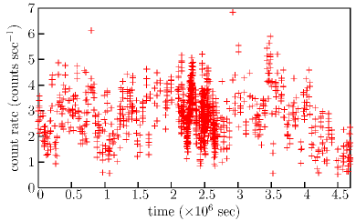
Figure 1: RXTE PCA light curve for NGC 4945 in the 8–30 keV band obtained in late 2002. Bin size is variable, with an average of 320 s. Error bars (not shown) are typically $\pm 0.3$ counts/s.

NGC 4945 was observed by RXTE in late 2002 for a period spanning a total of 50 days. A pointing of 1,400 seconds on average was scheduled approximately every 6 hours, while for 7 days centered within the total observation period the source was monitored intensively. Data from the Proportional Counter Array (PCA) were reduced using standard RXTE PCA analysis tools. The average count rate and the time-averaged photon spectrum are consistent with previous observations (Done, Madejski & Smith, 1996; Madejski et al., 2000). The nuclear flux below 8 keV is heavily absorbed at the source, presumably by the same material that is responsible for the megamaser activity. The counts from all three layers in PCU 0 and 2 corresponding to the nominal range of energies from 8 to 30 keV were added to produce a combined light curve (16 s intrinsic binning), resulting in a total of usable data of about 300 ks. The light curve is shown in figure 1.

2 Data analysis

The algorithm of Timmer & Koenig (1995) is used to generate simulated light curves based on a user-chosen PDS model that are then sampled to match the observation times of the source light curve. Further processing comprises subtracting the mean, scaling each light curve to the intrinsic variance of the source light curve, and adding random Gaussian numbers multiplied by the error bars of the source light curve. We then calculate the Lomb-Scargle periodogram (Lomb, 1976; Scargle, 1982) and re-bin it to 5 points per decade. Using the ensemble of (typically $>500$) simulated power density spectra, we fit the distribution of the periodogram power in each frequency bin with a stretched $\chi^{2}$ distribution: $p_{\nu}^{s}(\chi^{2},b)=b^{-1}p_{\nu}(\chi^{2}/b)$ where $p^{s}_{\nu}$ is the stretched, $p_{\nu}$ the regular $\chi^{2}$ distribution, $\nu$ is the number of DOF, and $b$ is the stretch factor. Finally, we compare the source periodogram to the fitted distributions, using a $\chi^{2}$-like statistic based on the likelihood ratio as the goodness-of-fit estimator (Baker & Cousins, 1984). The probability that an assumed model with the given set of parameters can be rejected is then the fraction of simulated light curves that have the likelihood ratio $\chi^{2}$ lower than the source light curve. The process is illustrated as a diagram in Fig. 2, but further explanation is outlined below.

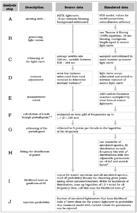
Figure 2: The diagram of the analysis steps used in the process of PDS characterization.
Footnotes to the diagram:
(1) error bar variance is calculated as the mean square of the source light curve error bars
(2) see Lomb (1976) and Scargle (1982)
(3) Since the rebinned light curve includes contiguous segments sampled at 320 sec resolution in the intensive section of the observation, information about the PDS shape can be extracted down to that timescale.
(4) We are only concerned here with finding a suitable parameterization of these distributions. $\chi^{2}$ distributions with a stretch factor are a natural choice since the power in the periodogram is drawn from $\chi^{2}$ distributions scaled by the power of the underlying PDS.

Scaling of simulated light curves to variance of source data (step D): In previous implementations of light curve simulations, the normalization of the PDS model was set to an arbitrary value at first. The best fit normalization was then determined by multiplying all simulated spectra by the same factor until the fit statistic was minimized (Markowitz et al., 2003; Uttley, McHardy & Papadakis, 2002). Due to the stochastic nature of the periodogram, the light curves simulated from a fixed normalization show a spread in variances (Vaughan et al., 2003), and the distribution of the power in each frequency bin will reflect this spread. By comparing the source data to a set of light curves simulated in this way, we are effectively asking the question: How well do the chosen shape and normalization of the PDS model describe the variability of the source? In reality, however, we are only interested in characterizing the shape of the periodogram. By allowing the normalization to vary from one light curve to the next, a slightly different question can be investigated: How likely is it that the source light curve was produced by a process that has the chosen PDS shape? By scaling each light curve to the intrinsic variance of the source light curve (and adding the Poisson noise level—see below), we ensure that the area under the curve for each simulated spectrum is equal to the one for the source.

Preservation of the Poisson noise level through the normalization of the PDS model (step E): The uncertainties in the source count rate are expected to contribute a constant level of power in the periodogram (usually called the Poisson noise level). Since the raw count rate in the RXTE PCA is dominated by the background for this source, the errors on the background-subtracted light-curve are approximately Gaussian. To mimic the effect of measurement errors in the simulated light curves, random Gaussian numbers multiplied by the error bars of the source light curve are added. This is done after the light curves have been scaled to the correct variance to ensure that the Poisson noise level in the simulated light-curves equals the one expected in the source data.

Use of robust fitting statistic to find best-fit parameters of the model PDS (steps H–J): A useful goodness-of-fit measure for non-Gaussian distributions is the rejection probability, calculated as the fraction of simulated light curves that have a value of the test statistic lower than the source data. The choice for test statistic is up to the investigator, and an obvious choice is the $\chi^{2}$ statistic, which uses the ensemble average and standard deviation of the power in each frequency bin for comparison to the source power. Because of the non-Gaussian nature of the distribution of power in each frequency bin, the applicability of the $\chi^{2}$ statistic is however severely limited: specifically, even small departures from Gaussian distributions have a marked effect on the standard deviation and thus on the rejection probability. Since the distribution of the power is more symmetric when plotted in the logarithm compared to the linear power, substantially different goodness-of-fit values can be obtained simply by a change of variable. The rejection probability, in effect, not only measures how well the model (and its associated parameters) describes the source data, but also the degree of non-Gaussianity. In contrast, by fitting the distributions of the power in each frequency bin with suitably parameterized functions (step H in the analysis), the effect of variable transformation on the fitting statistic is removed: If stretched $\chi^{2}$ distributions are an adequate description of the distribution of linear power, then under a change of variable the data can equally well be fit with the similarly transformed functions. The probability density for observing the source power as well as the value at the peak of the distribution is unchanged under these transformations. The likelihood ratio is thus an invariant quantity, i.e. independent of the chosen form of the variable used to describe the power in the periodogram.

3 Results

We investigated two models: the simple (unbroken) power law (power law slope as only parameter), and the knee model of Uttley, McHardy & Papadakis (2002) ($p(f)=A[1+(f/f_{b})^{2}]^{-\alpha/2}$; parameters: high frequency power law slope $\alpha$, break frequency $f_{b}$). Figures 3 and 4 show the rejection probabilities obtained. The unbroken power law results in a minimum rejection probability of 70% at a slope of 1.3, indicating a rather poor fit. The rejection probability is reduced to 40% by introducing a $10^{-6}$ Hz break at a high frequency slope of 1.5. It is clear that the exact location of the break is dependent on the particular PDS model used to characterize the source variability.

Uncertainty on rejection probability: To quantify the effect of simulating a finite number of light curves from which the goodness-of-fit statistic is estimated, we simulated more than 800,000 light curves using the unbroken power law model with a slope of 1.3. The process of fitting the distributions of power through calculating the rejection probability (steps H through J in Figure 2) was repeated for sets of light curves of increasing size. The mean of the distribution of rejection probabilities is consistent across the different sizes, while the standard deviation decreases from about 3% to 2.5% by going from 500 light curves to over 16,000. Assuming that the spread of rejection probabilities is only a weak function of the model and its associated parameters, we quote a characteristic uncertainty on our fitting statistic of about $\pm 3$%, based on 500 simulated light curves.

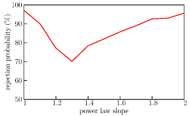
Figure 3: Rejection probability for the unbroken power law model, The best fit slope is 1.3, with a rejection probability of 70% indicating a poor fit.

Simple power law vs. knee model: The difference in rejection probability between the unbroken power law and the knee model is much larger than the above uncertainty. The flattening of the power towards low frequencies in NGC 4945 has thus been detected at a statistically significant level. The length of our observation is most likely not sufficient to distinguish between models that use different functional forms for the break in the PDS. In particular, the differences in rejection probabilities between the knee model and the broken power law model used in Uttley, McHardy & Papadakis (2002) is not expected to be statistically significant for the currently available light curve of NGC 4945.

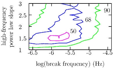
Figure 4: Rejection probability for the knee model, showing contours for 50, 68, and 90%. The best fit is obtained with a break frequency $f_{b}=10^{-6}$ Hz and a slope $\alpha=1.5$. The corresponding rejection probability is 40%.

References

- Papadakis & McHardy (1995) Papadakis, I., McHardy, I. 1995, MNRAS, 273, 923
- Edelson & Nandra (1999) Edelson, R., Nandra, K. 1999, ApJ, 514, 682
- Chiang et al. (2000) Chiang, J. et al. 2000, ApJ, 528, 292
- Nowak & Chiang (2000) Nowak, M., Chiang, J. 2000, ApJ, 531, L13
- Pounds et al. (2001) Pounds, K., Edelson, R., Markowitz, A., Vaughan, S. 2001, ApJ, 550, L15
- Markowitz et al. (2003) Markowitz, A. et al. 2003, ApJ, 593, 96
- McHardy et al. (2003) McHardy, I. M., Papadakis, I. E., Uttley, P., Page, M. J., Mason, K. O. 2003, MNRAS in press (astro-ph/0311220)
- Done et al. (1992) Done, C., Madejski, G. M., Mushotzky, R. F., Turner, T. J., Koyama, K., Kunieda, H. 1992, ApJ, 400, 138
- Uttley, McHardy & Papadakis (2002) Uttley, P., McHardy, I., Papadakis, I. 2002, MNRAS, 332, 231
- Czerny et al. (2003) Czerny, B., Doroshenko, V. T., Nikolajuk, M., Schwarzenberg-Czerny, A., Loska, Z., Madejski, G. 2003, MNRAS, 342, 1222
- Greenhill, Moran & Herrnstein (1997) Greenhill, L., Moran, J., Herrnstein, J. 1997, ApJ, 481, L23
- Done, Madejski & Smith (1996) Done, C., Madejski, G., Smith, D. 1996, ApJ 463, L63
- Madejski et al. (2000) Madejski, G., Zycki, P., Done, C., Valinia, A., Blanco, P., Rothschild, R., Turek, B. 2000, ApJ, 535, L87
- Timmer & Koenig (1995) Timmer, J., Koenig, M. 1995, A&A, 300, 707
- Lomb (1976) Lomb, N. R. 1976, Ap&SS, 39, 447
- Scargle (1982) Scargle, J. 1982, ApJ, 263, 835
- Baker & Cousins (1984) Baker, S., Cousins, R. D. 1984, Nucl. Instr. Meth. 221, 437
- Vaughan et al. (2003) Vaughan, S., Edelson, R., Warwick, R. S., Uttley, P. 2003, MNRAS, 345, 1271