Large-Scale Model of the Milky Way: Stellar Kinematics and Microlensing Event Timescale Distribution in the Galactic Bulge

Abstract

We build a stellar-dynamical model of the Milky Way barred bulge and disk, using a newly implemented adaptive particle method. The underlying mass model has been previously shown to match the Galactic near-infrared surface brightness as well as gas-kinematic observations. Here we show that the new stellar-dynamical model also matches the observed stellar kinematics in several bulge fields, and that its distribution of microlensing event timescales reproduces the observed timescale distribution of the MACHO experiment with a reasonable stellar mass function. The model is therefore an excellent basis for further studies of the Milky Way. We also predict the observational consequences of this mass function for parallax shifted events.

1 Introduction

It is now known, from several independent lines of evidence, that the Milky Way Galaxy (MWG) is barred (e.g., Gerhard (2001)). However, a comprehensive model consistent with the main observables – luminosity distribution, stellar-kinematics, gas-kinematics, and microlensing – has so far been still missing. Recently, Bissantz & Gerhard (2002) obtained a luminosity density model for the MWG from the dust-corrected $L$-band COBE/DIRBE map of Spergel, et al. (1995), through a non-parametric constrained maximum likelihood deprojection. This model (hereafter: COBE-$\rho$ model) is consistent also with the observed magnitude distributions of clump giant stars towards several bulge fields, and with the microlensing optical depth towards the bulge derived from these stars (Popowski, et al., 2003; Afonso, et al., 2003); see also Binney, et al. (2000) and Bissantz & Gerhard (2002). Furthermore Bissantz, et al. (2003) found that the hydrodynamical gas flow in the potential of the COBE-$\rho$ model matches the observed gas dynamics of the inner MWG well.

The structure of the inner MWG can also be constrained by observations of stellar kinematics along fixed lines of sight (Sharples, et al. (1990) [Sh90]; Spaenhauer, et al. (1992) [Sp92]; Minniti, et al. (1992) [Mi92]) and by the microlensing event timescale distribution (ETD) (Alcock, et al., 2000). The ETD has been studied largely with models which assume some distribution of disk and bulge kinematics (e.g. Han & Gould (1996); Peale (1998); Méra, et al. (1998)). An exception was Zhao, et al. (1996), who used the dynamical bar model of Zhao (1996) augmented by an analytic disk model, but failed to match the long duration ($\hat{t}>100$ days) tail of the ETD. In the present Letter we show that a full stellar-dynamical model based on the COBE-$\rho$ model is consistent with these independent data as well.

Dynamical models of the MWG have been generated using the Schwarzschild (1979) method, in which the distribution function (DF) of a galaxy is built from numerically integrated stellar orbits. Following earlier work by Zhao (1996), Häfner, et al. (2000) constructed a 22168-orbit dynamical model of the MWG. Dynamical models of the MWG have also been obtained by $N$-body methods (Fux, 1997). Syer & Tremaine (1996) [ST96] introduced a novel method for generating self-consistent dynamical models. The Syer-Tremaine (hereafter ST) method is allied to the Schwarzschild method, but, rather than superposing time-averaged observables from an orbit library, the ST method constructs a model by actively varying the weights of individual particles (orbits) as a function of time. This permits arbitrary geometry and a larger number of orbits to be used in the model building. Our dynamical model for the COBE-$\rho$ density in the MWG is constructed with the ST method, demonstrating its usefulness for real galaxy modeling. This Letter compares the model’s bulge kinematics and microlensing ETD with their observed counterparts.

2 The Syer-Tremaine method

The idea of the ST algorithm is to assign individual weights to particles of a simulation, which are then changed to reduce the deviation between the model and observations. An observable $Y_{j}$ associated to a stellar system characterized by a distribution function $f({\bf z})$, $\bf z=(x,v)$, can be written as $Y_{j}=\int K_{j}({\bf z})f({\bf z})d^{6}{\bf z}$, where $K_{j}({\bf z})$ is a known kernel. If this stellar system is simulated with $N$ particles having weights $w_{i}$ and phase space coordinates $\bf z_{i}$, then we can write the observables of the simulation as $y_{j}(t)=\sum_{i=1}^{N}w_{i}(t)K_{j}({\bf z_{i}}(t))$. ST96 define the ”force of change” on the weights as

$$\frac{dw_{i}(t)}{dt}=-\varepsilon w_{i}(t)\sum_{j}\frac{K_{j}({\bf z_{i}})}{Z_{j}}\left(\frac{y_{j}(t)}{Y_{j}}-1\right)$$ (1)

The small and positive parameter $\varepsilon$ governs how rapidly the weights are pushed such that the simulation observables $y_{j}(t)$ converge towards the observables $Y_{j}$. The constants $Z_{j}$ act as normalizations. The full ST method also includes prescriptions for temporal smoothing and a maximum entropy term, to reduce fluctuations. We have implemented the ST method with the MWG disk-plane surface density as the observable (Debattista et al. in preparation). We set $\varepsilon=0.25$, $\alpha=0.524$, $\mu=0.001$, where $\alpha$ and $\mu$ are the parameters of the temporal smoothing and the entropy terms, respectively, in the notation of ST96.

2.1 Simulation

Since the MWG contains a bar, our initial model also had to be barred. The simplest way to achieve this was to evolve an $N$-body model of an initially axisymmetric, bar-unstable, disk galaxy. The $N$-body simulation which produced the barred model consisted of live disk and bulge components inside a frozen halo. The frozen halo was represented by a cored logarithmic potential. The initially axisymmetric disk was modeled by a truncated exponential disk. Disk kinematics were set up using the epicyclic approximation to give Toomre $Q=1.3$. The disk and bulge were represented by $4\times 10^{6}$ equal-mass particles, with a mass ratio $M_{\rm d}:M_{\rm b}=4:1$. Further details of the setup methods and model units can be found in Debattista (2003) [D03]. We use the halo, disk, and bulge parameters given in Table 2 of D03, which give a flat rotation curve out to large radii.

The simulation was run on a 3-D cylindrical polar grid code (described in Sellwood & Valluri (1997)), with technical parameters exactly as in D03. The initially axisymmetric system was unstable and formed a rapidly rotating bar at $t\simeq 50$. By $t=160$, the bar instability had run its course and further secular evolution of the bar was mild. The resulting system did not match the COBE-$\rho$ model of the MWG and needed to be evolved further with the ST code. First, however, we eightfold symmetrized the COBE-$\rho$ model in order to reduce the amplitude of spirals, which we did not try to reproduce. We evolved the $N$-body model from $t=160$ under the ST prescription with the fixed potential of the COBE-$\rho$ model plus dark matter halo. We kept the bar pattern speed at its value in the $N$-body model, which scales to $56$ $\mathrm{km}~{}\mathrm{s}^{-1}~{}\mathrm{kpc}^{-1}$, consistent with the MWG (Dehnen (2000); Debattista, et al. (2002); Bissantz, et al. (2003)). At $t=240$ (i.e. $\simeq 4$ bar rotations), we shut off the ST algorithm and evolved the system to $t=280$ to assure that the particles are phase mixed.

3 Results: Density and Bulge Kinematics

To compare our dynamical COBE model (the COBE-Dyn model) with observations, we adopted the same viewing parameters as were used to determine the COBE-$\rho$ model: $R_{\odot}=8\,{\rm kpc},z_{\odot}=14{\rm pc}$ and $\varphi_{\rm bar}=20^{\circ}$ (Bissantz & Gerhard, 2002). We scale the velocities in the COBE-Dyn model to the MWG by matching to the local circular velocity. We assumed that the local standard of rest has only a circular motion, with $v_{LSR}=200$ $\mathrm{km}~{}\mathrm{s}^{-1}$, and we adopted the values of the solar peculiar motion from Dehnen & Binney (1998).

The densities of the COBE-Dyn and COBE-$\rho$ models match very well, with azimuthally averaged errors smaller than $5\%$ out to $R_{\odot}$. The largest errors ($<15\%$) occur in small isolated regions on the bar major-axis. In the (unconstrained) vertical direction, the disk is somewhat thicker than the MWG at $R_{\odot}$, but this leads to a change in optical depth $\tau$ towards Baade’s window of $<15\%$. In the bulge region, on the other hand, the scale-height of the COBE-Dyn model matches that of the MWG very well. We compared the model’s kinematics to observations towards Baade’s window (Sh90, Sp92) and in the field at $(l,b)=(8^{\circ},7^{\circ})$ (Mi92), using the selection functions determined by Häfner, et al. (2000). Table 1 shows our results. The overall fit of our model to the observed kinematics is rather good.

4 The Microlensing ETD

We now show that the COBE-Dyn model is also consistent with the microlensing ETD. Alcock, et al. (2000) presented an ETD, corrected for their experimental detection efficiency, based on 99 events in 8 fields. Popowski (2002) argued that one of these fields seems biased towards long-duration events, introducing some uncertainty in the observed ETD. Here we use the full-sample Alcock et al. ETD in order that our results may be compared with previous ones. We computed the ETD with the self-consistent kinematics of the COBE-Dyn model. A microlensing event is characterized by the source distance, $D_{S}$, lens distance, $D_{L}$, the proper motion, $v_{\perp}$, of the lens with respect to the line-of-sight between observer and source, and lens mass, $M_{L}$. The probability $P(\hat{t})$ for observing an event duration $\hat{t}=2\Theta_{E}/v_{\perp}$ is given by

$$P(\hat{t})\propto\int\rho(D_{S})D_{S}^{2+2\beta}\rho(D_{L})D_{L}^{2}\Theta_{E}(D_{S},D_{L},M_{L})$$

$$\Phi(M_{L})v_{\perp}f(v_{\perp})\delta(\hat{t}-2\Theta_{E}/v_{\perp})dv_{\perp}~{}dD_{L}~{}dD_{S}~{}dM_{L}.$$ (2)

Here $\rho(d)$ is the density of the MWG at distance $d$ from the observer along the line-of-sight to the observed field, $\Phi(M_{L})$ is the mass function (MF) of the lens population, $\Theta_{E}(D_{S},D_{L},M_{L})$ is the Einstein angle, and $f(v_{\perp})$ is the distribution of $v_{\perp}$. We solved the multiple integral by Monte Carlo random drawings of the parameters $(D_{S},D_{L},v_{\perp},M_{L})$ as follows: (1) To obtain the source distance ($0\leq D_{S}\leq D_{S}^{\rm max}=12\,{\rm kpc}$), we used the COBE-$\rho$ model, since this is less noisy than the particle realization. The probability of $D_{S}$ is $\propto\rho(D_{S})D_{S}^{2+2\beta}$ with $\beta\!=\!-1$, to account for a magnitude cut-off (Kiraga & Paczyński, 1994). (2) The lens distance ($0\leq D_{L}<D_{S}$) was selected from $\tilde{\rho}(D_{L})\int_{0}^{D_{S}}\rho(D_{L})dD_{L}$, where $\tilde{\rho}$ is a normalized probability density distributed as in the COBE-$\rho$ model. (3) For the relative velocity $v_{\perp}$, we used the particle distribution of the COBE-Dyn model, randomly selecting a particle at $\sim D_{S}$ and another at $\sim D_{L}$. The proper motions of these particles then determined $v_{\perp}$. (4) The lens mass $M_{L}/M_{\odot}$ was selected from a Kroupa (1995) MF, $\Phi(M_{L})=\beta(M_{L}/M_{\odot})^{-\gamma}$, with

$$(\gamma,\beta)=\cases{\displaystyle(2.35,0.1038)&$M_{L}^{<}\leq M_{L}/M_{\odot}\leq 0.35$\cr(0.6,0.6529)&$0.35\leq M_{L}/M_{\odot}\leq 0.6$\cr(2.35,0.2674)&$0.6\leq M_{L}/M_{\odot}\leq M_{L}^{>}$\cr}$$ (3)

We explored varying $M_{L}^{<}$ and $M_{L}^{>}$. We obtained the ETD, shown in Fig. 1, by simulating $10^{5}$ events, and weighting each by the remaining factors in Eqn. 2. We tested our Monte Carlo integrations by reproducing one of Peale (1998)’s model ETDs.

We started with $(M_{L}^{<},M_{L}^{>})=(0.075,10)$, for which we obtained a Kolmogorov-Smirnov distance between data and model of $D_{KS}=0.213$. (We excluded the bin at $\hat{t}<3.1$ days from the MACHO data in all such comparisons, because it appears to be too heavily affected by its large detection-efficiency correction.) To improve on this fit, we first explored the effects of uncertainties in the COBE-$\rho$ model. The most important of these is $\varphi_{\rm bar}$. Setting $\varphi_{\rm bar}=30^{\circ}$, we found only a minor change to the ETD, in agreement with Peale (1998). Making the bar stronger, or the disk velocity dispersion outside the bar smaller did not alter the ETD substantially. Therefore we next explored variations in the MF. Like Peale (1998), we found that modest changes can improve the fit substantially. Our best fit, with $D_{KS}=0.068$ was obtained with $M_{L}^{<}=0.04$ and $M_{L}^{>}=10$. However, a more conservative limit is $M_{L}^{>}=4$, which gives $D_{KS}=0.081$. (If the suggestion of Popowski (2002) is correct, which would shift the ETD peak to smaller $\hat{t}$, then a smaller $M_{L}^{>}$ would be required anyway.)

We now explore the causes of long duration (LD) events in the COBE-Dyn model; using $(M_{L}^{<},M_{L}^{>})=(0.04,4)$ as our standard model for this analysis. We start by noting, from Fig. 1, that the vast majority of sources are located in the bulge ($6\leq D_{S}\leq 10$ kpc). This is also true for the lenses responsible for short duration events, but disk lenses become more important at longer durations; indeed, for ${\hat{t}}>25$ days, one third of the lenses are at $D_{L}<4$ kpc. In Fig. 2 we separate the ETD into the near and distant lens sub-samples and show the heliocentric angular velocities and cumulative distributions of $M_{L}$ for both. Note first that lenses with $M_{L}>0.5M_{\odot}$ contribute significantly to LD events in both the near and distant sub-samples. Lens mass, however, is not the full explanation of the LD events, as has been noted by previous studies, and the relative motions of lens and source in the heliocentric frame must also be considered. The kinematics of the LD sources are substantially those of a rotating triaxial bulge/bar which points almost towards the observer: thus their apparent tangential motions are largely due to the solar motion, giving $\Omega_{tan,S}\sim 205/8$ $\mathrm{km}~{}\mathrm{s}^{-1}~{}\mathrm{kpc}^{-1}$. Distant lens LD events are then possible because the lenses share very similar kinematics with the sources (note that massive lenses become necessary only in the last quartile, $\hat{t}>60$ days). For the nearby lens sample, LD events have a rather large spread in $\Omega_{tan,L}$ (due both to their proximity and the velocity dispersion of the COBE-Dyn model), which together with larger $M_{L}$’s is able to produce LD events. We conclude, therefore, that there is no single cause for the long-duration events.

Standard 3-parameter fits to microlensing events are symmetric about the time of peak amplification, resulting in a degeneracy between $M_{L}$, $v_{\perp}$, $D_{L}$ and $D_{S}$. One degree of degeneracy is removed by also measuring the light-curve shift due to the parallax from earth’s orbit, which gives a relation between $v_{\perp}$ and $D_{L}/D_{S}$. These shifts are present in all events, but most go undetected because of infrequent sampling and photometric errors. Buchalter & Kamionkowski (1997) estimate a $1\%$ detection efficiency of parallax-shifted events for the MACHO-type setup, and much higher for second generation experiments. The light curves of such events require 5 parameters, including $\kappa\equiv R_{\oplus}(D_{L}^{-1}-D_{S}^{-1})/\Theta_{E}$, where $R_{\oplus}=1$ AU. In Fig. 3, we present our predictions for the probability distribution in the $(\kappa,\hat{t})$-plane, assuming $100\%$ detection efficiency. These distributions are twin-peaked, with the lower peak increasingly separated from the global peak as $M_{L}^{<}$ decreases, as it must since $\kappa\propto\Theta_{E}^{-1}$ while $\hat{t}\propto\Theta_{E}$. The location of the second peak may therefore provide an observational constraint on the MF at low mass.

5 Conclusions

We have presented a dynamical model of the MWG constructed using the Syer-Tremaine method, constrained only by the MWG density map of Bissantz & Gerhard (2002). Although no kinematic constraints were used, the model (i) matches observed bulge kinematics in several fields and is (ii) able to reproduce the observed microlensing event timescale distribution. For the best fitting MF, the model (iii) predicts a twin-peaked probability distribution in the $(\kappa,\hat{t})$-plane, which may be observationally tested with new generations of microlensing experiments. (iv) The underlying mass model has been previously shown to match the Galactic near-infrared surface brightness as well as gas-kinematic observations. It is therefore an excellent basis for further studies of the Milky Way.

	$(l,b)$	Ref.	Observed	COBE-Dyn
$v^{h}_{\rm los}$	$(1^{\circ},-4^{\circ})$	Sh90	$4\pm 8$	8.2
$\sigma_{\rm los}$	$(1^{\circ},-4^{\circ})$	Sh90	$113\pm 5$	109
$\sigma_{\rm los}$	$(1^{\circ},-4^{\circ})$	Sp92	$120$	109
$\sigma^{h}_{\mu_{l}}$	$(1^{\circ},-4^{\circ})$	Sp92	$3.2\pm 0.1$	3.1
$\sigma^{h}_{\mu_{b}}$	$(1^{\circ},-4^{\circ})$	Sp92	$2.8\pm 0.1$	2.4
$v^{g}_{\rm los}$	$(8^{\circ},7^{\circ})$	Mi92	$45\pm 10$	46
$\sigma_{\rm los}$	$(8^{\circ},7^{\circ})$	Mi92	$85\pm 7$	100

Table 1: Comparison of kinematic quantities computed from the COBE-Dyn model with observations. In the first column, the superscript ^h indicates that the value given is heliocentric, and ^g that it is Galactocentric. All quantities are in $\mathrm{km}~{}\mathrm{s}^{-1}$ except for $\sigma^{h}_{\mu_{l}}$ and $\sigma^{h}_{\mu_{b}}$, which are in milliarcseconds year${}^{-1}.$

Figure Captions

Fig. 1 The ETD of the COBE-Dyn model compared to the detection-efficiency-corrected observations of the MACHO group (histograms in all panels). Top: cumulative distribution function for the standard model, $(M_{L}^{<},M_{L}^{>})=(0.04,4)$, (solid line), the best model with $(M_{L}^{<},M_{L}^{>})=(0.04,10)$ (dotted), and a model with $(M_{L}^{<},M_{L}^{>})=(0.075,10)$ (dashed). We obtain $D_{KS}=0.081,0.068,0.213$, respectively, for the 3 models. Middle panel: differential distributions of these models (same line styles). (In these two panels, all model distributions have been smoothed with a kernel density estimator of bandwidth $0.1$.) Bottom: ETD of the $(M_{L}^{<},M_{L}^{>})=(0.04,4)$ model and its decomposition into events with: $6\leq D_{S}\leq 10$ kpc (dotted line), $0\leq D_{L}\leq 4$ kpc (dashed) and $D_{L}>4$ kpc (dot-dashed).

Fig. 2 Top two panels: The long duration events ($\hat{t}>42$ days) in the $(M_{L}^{<},M_{L}^{>})=(0.04,4)$ model. Both are maps (on the same relative scale) in the plane of heliocentric tangential angular velocities, $\Omega_{tan,L}$ and $\Omega_{tan,S}$. Left: near lenses ($D_{L}<4$ kpc); right: distant ones ($D_{L}>4$ kpc). The diagonal and horizontal dashed lines indicate $\Omega_{tan,L}=\Omega_{tan,S}$ and $\Omega_{tan,S}=205/8=25.6$ $\mathrm{km}~{}\mathrm{s}^{-1}~{}\mathrm{kpc}^{-1}$, respectively. Bottom: distributions of $M_{L}$ for distant (solid lines) and nearby (dashed) lenses. The different lines result from splitting into quartiles by contribution to the full ETD the distribution of events sorted on $\hat{t}$. Event durations increase as the mean mass increases. The heavy curve shows the underlying mass function.

Fig. 3 Predicted probability distribution of parallax shifted events in the $(\kappa,\hat{t})$-plane, for the standard model with $(M_{L}^{<},M_{L}^{>})=(0.04,4)$. We use a smoothing kernel with $(\delta_{\kappa},\delta_{\log\hat{t}})=(0.01,0.1)$. The stars mark the locations of secondary peaks when $M_{L}^{<}=$ 0.075, 0.04, 0.02 and 0.01 in order of increasing $\kappa$.

Figure 1:

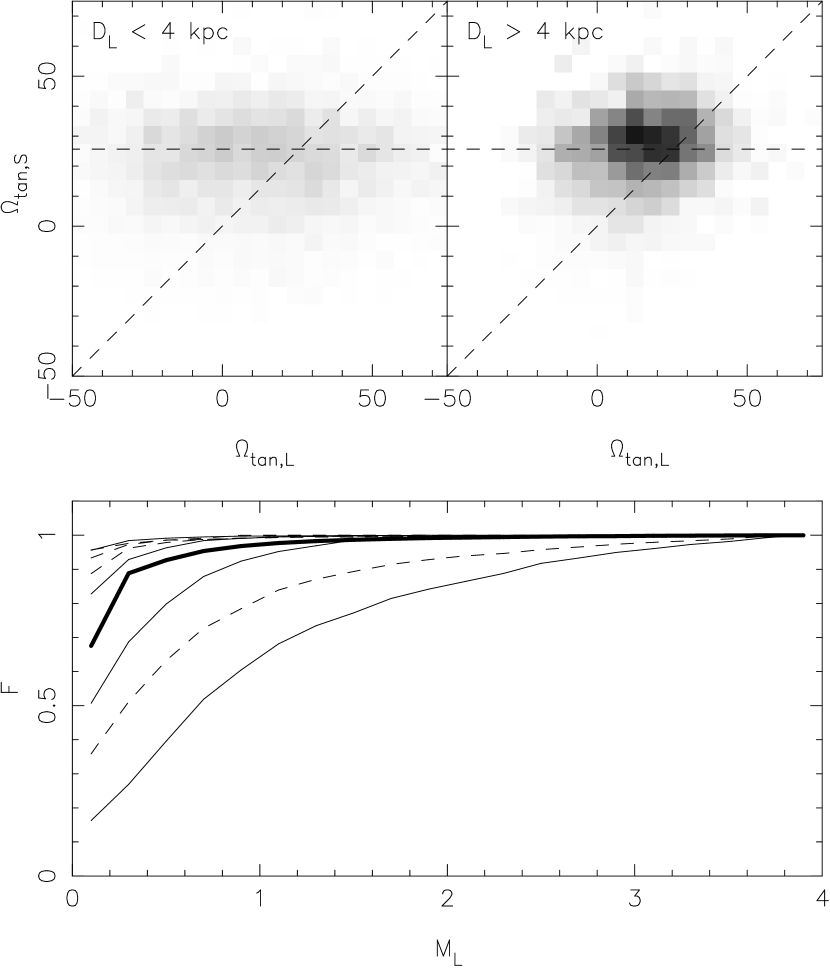
Figure 2:

Figure 3:

References

- Afonso, et al. (2003) Afonso, C., et al. 2003, A&A, 404, 145
- Alcock, et al. (2000) Alcock, C., et al. 2000, ApJ, 541, 734
- Binney, et al. (2000) Binney, J. J., Bissantz, N., Gerhard, O. E. 2000, ApJL, 537, L99
- Bissantz, et al. (2003) Bissantz, N., Englmaier, P., Gerhard, O. E. 2003, MNRAS, 340, 949
- Bissantz & Gerhard (2002) Bissantz, N., Gerhard, O. E. 2002, MNRAS, 330, 591
- Buchalter & Kamionkowski (1997) Buchalter, A., Kamionkowski, M. 1997, ApJ, 482, 782
- Debattista, et al. (2002) Debattista, V. P., Gerhard, O., & Sevenster, M. N. 2002, MNRAS, 334, 355
- Debattista (2003) Debattista, V. P. 2003, MNRAS, 342, 1194 [D03]
- Dehnen (2000) Dehnen, W. 2000, AJ, 119, 800
- Dehnen & Binney (1998) Dehnen, W., Binney, J. 1998, MNRAS, 298, 387
- Fux (1997) Fux, R. 1997, A&A, 327, 983
- Gerhard (2001) Gerhard O. 2001, in Galaxy Disks and Disks Galaxies, ed. J. G. Funes, S.J. & E. M. Corsini, (San Francisco: ASP Conf series 230), pg. 21
- Häfner, et al. (2000) Häfner, R., Evans, N. W., Dehnen, W., Binney, J. 2000, MNRAS, 314, 433
- Han & Gould (1996) Han, C., Gould, A. 1996, ApJ, 473, 230
- Kiraga & Paczyński (1994) Kiraga, M., Paczyński, B. 1994, ApJ, 430, L101
- Kroupa (1995) Kroupa, P. 1995, ApJ, 453, 358
- Méra, et al. (1998) Méra, D., Chabrier, G., Schaeffer, R. 1998, A&A, 330, 937
- Minniti, et al. (1992) Minniti, D., White, S. D. M., Olszewski, E. W., Hill, J. M. 1992, ApJ, 393, 47 [Mi92]
- Peale (1998) Peale, S. J. 1998, ApJ, 509, 177
- Popowski, et al. (2003) Popowski, P. et al. 2003, in Gravitational lensing: a unique tool for cosmology, Aussois 2003, eds. D. Valls-Gabaud & J.-P. Kneib, in press, astro-ph/0304464
- Popowski (2002) Popowski, P. 2002, MNRAS, submitted astro-ph/0205044
- Schwarzschild (1979) Schwarzschild, M. 1979, ApJ, 232, 236
- Sellwood & Valluri (1997) Sellwood, J. A., Valluri M. 1997, MNRAS, 287, 124
- Sharples, et al. (1990) Sharples, R., Walker, A., Cropper, M. 1990, MNRAS, 246, 54 [Sh90]
- Spaenhauer, et al. (1992) Spaenhauer, A., Jones, B. F., Whitford, A. E. 1992, AJ, 103, 297 [Sp92]
- Spergel, et al. (1995) Spergel, D. N., Malhotra, S., Blitz, L. 1995 Proc. ESO/MPA Workshop on Spiral Galaxies in the Near-IR, D. Minniti, H.-W. Rix (eds.), Springer 1996
- Syer & Tremaine (1996) Syer, D., Tremaine, S. 1996, MNRAS, 282, 223
- Zhao (1996) Zhao, H.-S. 1996, MNRAS, 283, 149
- Zhao, et al. (1996) Zhao, H.-S., Rich, R. M., Spergel, D. N. 1996, MNRAS, 282, 175