Accretion onto a primordial protostar

Abstract

We present a three-dimensional numerical simulation that resolves the formation process of a Population III star down to a scale of $\sim 100$ AU. The simulation is initialized on the scale of a dark matter halo of mass $\sim 10^{6}M_{\odot}$ that virializes at $z\sim 20$. It then follows the formation of a fully-molecular central core, and traces the accretion from the diffuse dust-free cloud onto the protostellar core for as long as $\sim 10^{4}$ yr, at which time the core has grown to $\sim 50M_{\odot}$. We find that the accretion rate starts very high, $\sim 0.1M_{\odot}\mbox{\,yr}^{-1}$, and declines rapidly thereafter approaching a power-law temporal scaling. Asymptotically, at times $t\gtrsim 10^{3}\mbox{\,yr}$ after core formation, the stellar mass grows approximately as $M_{\ast}\simeq 20M_{\odot}(t/10^{3}\mbox{\,yr})^{0.4}$. Earlier on, accretion is faster with $M_{\ast}\propto t^{0.75}$. By extrapolating this growth over the full lifetime of very massive stars, $t\simeq 3\times 10^{6}$ yr, we obtain the conservative upper limit $M_{\ast}\lesssim 500M_{\odot}$. The actual stellar mass is, however, likely to be significantly smaller than this mass limit due to radiative and mechanical feedback from the protostar.

,

1 Introduction

The first (so-called Population III) stars could have had a dramatic influence on the early universe at redshifts $z\lesssim 20$. Their high yield of ionizing photons may have reionized the intergalactic medium (IGM) (e.g., Cen, 2003; Ciardi et al., 2003; Haiman and Holder, 2003; Sokasian et al., 2003; Somerville and Livio, 2003; Wyithe and Loeb, 2003). In addition, the first supernovae (SNe) were responsible for the initial IGM metal-enrichment (e.g., Madau et al., 2001; Mori et al., 2002; Schneider et al., 2002; Bromm et al., 2003; Furlanetto and Loeb, 2003; Mackey et al., 2003; Scannapieco et al., 2003; Wada and Venkatesan, 2003; Norman et al., 2004; Yoshida et al., 2004). The radiative and hydrodynamic feedback of the first stars affected subsequent galaxy formation (Barkana and Loeb, 2001) and imprinted large-scale polarization anisotropies on the cosmic microwave background (Kaplinghat et al., 2003; Kogut et al., 2003). In the context of popular cold dark matter (CDM) models of hierarchical structure formation, the first stars are predicted to have formed in dark matter halos of mass $\sim 10^{6}M_{\odot}$ that collapsed at redshifts $z\simeq 20-30$ (e.g., Tegmark et al., 1997; Barkana and Loeb, 2001; Yoshida et al., 2003). Since their ionization efficiency (Tumlinson and Shull, 2000; Bromm et al., 2001; Schaerer, 2002) and metal yield (Heger and Woosley, 2002; Umeda and Nomoto, 2002, 2003) depends on their mass, the fundamental question is (e.g., Bromm, 2004): How massive were the first stars?

Results from recent numerical simulations of the collapse and fragmentation of primordial clouds suggest that the first stars were predominantly very massive, with typical masses $M_{\ast}\gtrsim 100M_{\odot}$ (Bromm et al., 1999, 2002; Nakamura and Umemura, 2001; Abel et al., 2002). More specifically, these simulations have identified pre-stellar clumps of masses up to $\sim 10^{3}M_{\odot}$ and sizes $\lesssim 0.5$ pc. Each of the simulated clumps is conjectured to be the immediate progenitor of a single star or a small cluster of stars (see Larson 2003 for a review). To determine the mass of a single star, one must follow the fate of such a clump. Extending the analogous calculation for the collapse of a present-day protostar (Larson, 1969) to the primordial case, Omukai and Nishi (1998) have carried out one-dimensional hydrodynamical simulations in spherical symmetry. They have found that the mass of the initial hydrostatic core, formed near the center of the collapsing cloud when the density is sufficiently high ($n\sim 10^{22}$ cm^-3) for the gas to become optically thick to continuum radiation, is almost the same as in present-day star formation: $M_{\rm core}\sim 5\times 10^{-3}M_{\odot}$. The small value of the initial core has no bearing on the final mass, which is in turn determined by how efficient the accretion process is at incorporating the clump mass into the growing protostar.

In this paper, we present results from the first three-dimensional simulation that is initialized on cosmological scales, followed to the formation of a protostellar high-density core, and for which the accretion flow is traced onto the central protostar for as long as $\sim 10^{4}$ yr after core formation. We do not yet self-consistently take into account the radiative and mechanical feedback from the protostar on the accretion flow (Omukai and Palla, 2001, 2003; Tan and McKee, 2003). By comparing to one-dimensional calculations that address this feedback on the accretion flow, we demonstrate that the accretion process is likely to lead to the formation of large stellar masses, as conjectured before.

Throughout this paper, we assume a standard $\Lambda$CDM cosmology, with a total density parameter in matter of $\Omega_{m}=1-\Omega_{\Lambda}=0.3$, and in baryons of $\Omega_{\rm B}=0.045$, a Hubble constant $h=H_{0}/(100$ km s^-1 Mpc${}^{-1})=0.7$, and a power-spectrum amplitude $\sigma_{8}=0.9$ on $8h^{-1}$Mpc spheres. These values reflect the latest estimates of cosmological parameters from the Wilkinson Microwave Anisotropy Probe (WMAP) (Spergel et al., 2003).

2 Physical ingredients

The main physical processes operating prior to the formation of a pre-stellar clump with typical mass of a few hundred solar masses are described in earlier work (Bromm et al., 2002; hereafter BCL). Below we discuss the physical effects that become important during the subsequent collapse to higher densities and the resultant formation of a protostellar core (see also Bromm, 2000).

The formation of hydrogen molecules due to the H^- channel saturates at a fractional abundance of $\sim 10^{-3}$ (BCL). At densities exceeding $\sim 10^{8}$ cm^-3, however, three-body reactions are able to convert the gas into an almost fully molecular form (Palla et al., 1983). In addition to the reactions discussed by BCL (see their Table 1), we also consider here

$$(13)\mbox{\ \ \ \ }\mbox{H}+\mbox{H}+\mbox{H}\rightarrow\mbox{H}_{2}+\mbox{H}$$

$$(14)\mbox{\ \ \ \ }\mbox{H}+\mbox{H}+\mbox{H}_{2}\rightarrow\mbox{H}_{2}+\mbox{H}_{2}$$

The reaction rates are (Palla et al., 1983): $k_{13}=5.5\times 10^{-29}(T/{\rm K})^{-1}$ cm⁶ s^-1, and $k_{14}=\frac{1}{8}k_{13}$. To estimate the density at which three-body reactions become important, we consider reaction (13)

$$\frac{\mbox{d}n{\mbox{\scriptsize[H${}_{2}$]}}}{\mbox{d}t}=k_{13}\left(n\mbox{\scriptsize[H]}\right)^{3}\mbox{\ \ \ .}$$ (1)

Defining the fractional abundance of H₂ molecules as $f=2n\mbox{\scriptsize[H${}_{2}$]}/n_{\mbox{\scriptsize H}}$, and expressing the density of hydrogen atoms $n\mbox{\scriptsize[H]}=(1-f)n_{\mbox{\scriptsize H}}$ with $f\sim 10^{-3}\ll 1$, we get the timescale for reaction (13)

$$t_{\mbox{\scriptsize 3-body}}\simeq\frac{f}{2k_{13}n^{2}_{\rm H}}.$$ (2)

The value of $t_{\mbox{\scriptsize 3-body}}$ equals the free-fall timescale at a critical density

$$n_{\rm H}\simeq\left(\frac{f^{2}Gm_{\rm H}}{4k_{13}^{2}}\right)^{1/3}\mbox{\ \ \ .}$$ (3)

Evaluating $k_{13}$ at $T\simeq 10^{3}$ K, and assuming $f\simeq 10^{-3}$, we find that three-body reactions set in at $n_{\rm H}\simeq 2\times 10^{8}$ cm^-3. Along similar lines, by considering reaction (14) and assuming $f\simeq 0.5$, we find that the density at which the conversion of hydrogen atoms into molecules is complete is $n_{\rm H}\simeq 5\times 10^{11}$ cm^-3. Both estimates are in good agreement with our numerical results. The transformation of the hydrogen gas from an atomic phase to a molecular phase requires three modifications of the physics incorporated in the numerical code as described below (see also Omukai and Nishi, 1998).

First, the heating associated with the formation of H₂ and the corresponding release of the molecular binding energy, $\epsilon_{\rm H_{2}}=4.48$ eV, becomes important at high densities. To account for this additional heating source, we add to the energy equation (see BCL) the term (in ergs s^-1 cm^-3)

$$\Gamma_{\mbox{\scriptsize 3-body}}=\epsilon_{\rm H_{2}}\frac{\mbox{d}n{\mbox{\scriptsize[H${}_{2}$]}}}{\mbox{d}t}\mbox{\ \ \ ,}$$ (4)

for densities $n_{\rm H}\geq 10^{8}$ cm^-3.

Second, the H₂ cooling function has to be augmented to include both the collisional excitation of H₂ by H atoms and by H₂ molecules. The total cooling rate (in ergs s^-1 cm^-3) can then be written as

$$\Lambda=n^{2}_{\rm H}f\left[\frac{n\mbox{\scriptsize[H]}}{n_{\rm H}}L^{\rm H}+fL^{\rm H_{2}}\right]\mbox{\ \ \ ,}$$ (5)

where $L^{\rm H}$ and $L^{\rm H_{2}}$ (in erg s^-1 cm³) are the vibrational/rotational cooling coefficients for collisions with H atoms and H₂ molecules, respectively. At the high densities considered here, all levels are close to being populated according to local thermodynamic equilibrium (LTE). For $L^{\rm H}$ and $L^{\rm H_{2}}$, we use the parameterization given by Hollenbach and McKee (1979).

Third, the presence of molecules leads to a modified equation of state. We write the gas pressure as

$$P=\frac{k_{\rm B}T}{\mu m_{\rm H}}\rho=(\gamma_{\rm ad}-1)\rho u\mbox{\ \ \ ,}$$ (6)

where $\gamma_{\rm ad}$ is the adiabatic exponent, and $u$ is the specific internal energy. The mean molecular weight, $\mu$, is given by

$$\frac{1}{\mu}=\frac{Y}{4}+(1-f)X+f\frac{X}{2}\mbox{\ \ \ ,}$$ (7)

where $X=0.76$ and $Y=1-X$ are the mass fractions in hydrogen and helium, respectively. For a gas consisting of helium and pure atomic hydrogen, $\mu\simeq 1.22$, whereas for a mixture of helium and pure molecular hydrogen, $\mu\simeq 2.27$. The adiabatic exponent can be expressed as

$$\gamma_{\rm ad}-1=\frac{1}{\mu}\left(\sum_{i}\frac{1}{(\gamma_{i}-1)\mu_{i}}\right)^{-1}\mbox{\ \ \ ,}$$ (8)

where the summation is over the 6 species H, H⁺, H^-, H₂, e^-, and He, with $\mu_{\rm H_{2}}=2$, $\mu_{\rm He}=4$, and $\mu_{i}=1$ otherwise. In calculating the adiabatic exponent for H₂, one has to consider translational, rotational, and vibrational degrees of freedom, resulting in

$$\frac{1}{\gamma_{\rm H_{2}}-1}=\frac{1}{2}\left(3+2+\frac{2\bar{\epsilon}_{\rm vib}}{k_{\rm B}T}\right)\mbox{\ \ \ .}$$ (9)

Here, $\bar{\epsilon}_{\rm vib}$ is the average vibrational energy per H₂ molecule, and is given by (e.g., Shu, 1991)

$$\bar{\epsilon}_{\rm vib}=\frac{\hbar\omega_{0}}{{\rm e}^{\hbar\omega_{0}/k_{\rm B}T}-1}+\frac{1}{2}\hbar\omega_{0}\mbox{\ \ \ ,}$$ (10)

with $\hbar\omega_{0}/k_{\rm B}\simeq 6300$ K. For the physical conditions considered here, the excitation of vibrational degrees of freedom is never important. Other non-molecular species have only translational degrees of freedom, and consequently, $1/(\gamma_{i}-1)=3/2$. We terminate the simulation when the central density is sufficiently high for opacity effects to be important. In the following, we estimate analytically the density beyond which the H₂ line radiation cannot escape from the central fully-molecular core of the gas.

Molecular opacity starts to affect the cooling rate of the gas at a sufficiently high density. At temperatures $T\sim 10^{3}$ K, only the rotational transitions within the lowest-lying vibrational level contribute significantly to the cooling. Taking into account the quadrupole nature of the transitions, corresponding to the selection rule $\Delta J=2$ (where $J$ is the angular momentum quantum number), one may express the H₂ cooling function as

$$\Lambda=\sum_{J\rightarrow J-2}n_{J}A_{J,J-2}\Delta E_{J,J-2}\mbox{\ \ \ .}$$ (11)

The number density of molecules in rotational level $J$ is given by

$$n_{J}=\frac{n\mbox{\scriptsize[H${}_{2}$]}}{Z}(2J+1)\mbox{e}^{-E_{J}/k_{\rm B}T}\mbox{\ \ \ ,}$$ (12)

where $n\mbox{\scriptsize[H${}_{2}$]}$ is the total H₂ number density, $E_{J}=85.3\mbox{\,K\ }J(J+1)$ is the energy corresponding to level $J$, and $Z$ is the partition function

$$Z=\sum_{J=0}^{\infty}(2J+1)\mbox{e}^{-E_{J}/k_{\rm B}T}\mbox{\ \ \ .}$$ (13)

The energy difference between levels $J$ and $J-2$ is $\Delta E_{J,J-2}$, and the corresponding probability per unit time for spontaneous emission is $A_{J,J-2}\propto\Delta E_{J,J-2}^{5}$. We first identify the transition that dominates the radiative cooling at a given temperature, and then determine the opacity in this most important line. The most important transition is near the extremum set by the condition

$$\frac{\mbox{d}}{\mbox{d}J}(n_{J}A_{J,J-2}\Delta E_{J,J-2})=0\mbox{\ \ \ ,}$$ (14)

implying

$$J_{\rm max}\simeq 6.4\left(\frac{T}{\mbox{1000\,K}}\right)^{1/2}\mbox{\ \ \ ,}$$ (15)

where $T\sim 10^{3}$ K is typical for the central region of the collapsing clump.

For the $6\rightarrow 4$ transition, the line absorption coefficient (in cm^-1) can be expressed as (Rybicki and Lightman, 1979)

$$\alpha_{\nu}=\frac{\Delta E_{6,4}}{4\pi}n_{4}B_{4,6}\left[1-\mbox{e}^{-\Delta E_{6,4}/k_{\rm B}T}\right]\varphi(\nu)\mbox{\ \ \ ,}$$ (16)

where we have taken the levels to be populated according to LTE. By assuming that broadening is entirely due to the thermal Doppler effect, the profile function is

$$\varphi(\nu)=\frac{1}{\sqrt{\pi}\Delta\nu_{D}}\exp\left[-\frac{(\nu-\nu_{0})^{2}}{\Delta\nu_{D}^{2}}\right]\mbox{\ \ \ ,}$$ (17)

with $\Delta\nu_{D}=(\nu_{0}/c)\sqrt{2k_{\rm B}T/m}$, a particle mass $m=2m_{\rm H}$ for H₂, and $h\nu_{0}=\Delta E_{6,4}$. This function leads to a modest overestimate of the opacity, as parts of the accretion flow are mildly supersonic (with a maximum Mach number of $\sim 1.5$ at radius $\sim 200$ AU), but our goal here is only to get a rough estimate as to when line opacity becomes important. In the following, we approximate $\varphi(\nu)\sim\varphi(\nu_{0})=1/(\sqrt{\pi}\Delta\nu_{D})$, and use $\Delta\nu_{D}/\nu_{0}\simeq 10^{-5}$ for $T\sim 10^{3}$ K. The Einstein coefficient for stimulated absorption is

$$B_{4,6}=\frac{13}{9}\frac{c^{2}h^{2}}{2(\Delta E_{6,4})^{3}}A_{6,4}\simeq 0.04{\rm\ cm}^{2}{\rm\ erg}^{-1}{\rm\ s}^{-1}\mbox{\ \ ,}$$ (18)

where $A_{6,4}$ is taken from Turner et al. (1977). At $T\sim 10^{3}$ K, the partition function is $Z\simeq 12.1$, and using equation (15) we find $n_{4}\simeq 0.1n\mbox{\scriptsize[H${}_{2}$]}$.

We may now estimate the density at which the optical depth, $\tau_{\nu}\simeq\alpha_{\nu}L$, approaches unity, where $L$ is the characteristic size of the high-density, fully molecular region

$$n_{\rm H}\simeq 3\times 10^{6}\mbox{\,cm${}^{-3}$\,}\left(\frac{L}{\mbox{pc}}\right)^{-1}\mbox{\ \ \ .}$$ (19)

From our simulation, we estimate $L\simeq 10^{-4}$ pc, and consequently have $n_{\rm H}\simeq 10^{11}$ cm^-3. At densities exceeding this value, radiation can still escape in less opaque lines with a smaller $A$ coefficient, and in the continuum between the lines, but neglecting the effects of radiative transfer renders the results of the simulation increasingly unreliable at yet higher densities. Omukai and Nishi (1998), who did include the treatment of radiative transfer, were able to follow the collapse all the way to stellar densities, although their approach was limited to a spherical geometry. In our numerical simulation, we form a sink particle once the gas density exceeds a value of $10^{12}$ cm^-3 (see BCL for details about the numerical implementation). This sink particle approximates a hydrostatic core at the center of the accretion flow, although it has a size that is still much larger than the expected scale of the actual core (Omukai and Nishi, 1998; Ripamonti et al., 2002).

3 Numerical methodology

The evolution of the dark matter and gas components is calculated with a version of TREESPH (Hernquist and Katz, 1989), combining the smoothed particle hydrodynamics (SPH) method with a hierarchical (tree) gravity solver (see BCL for further details). Here, we briefly describe the modifications introduced to the code in order to allow it to treat accretion flows in a dense, high-redshift environment.

We initialize the simulation (see § 4.1) on the scale of the minihalo ($\gtrsim 150$ pc), and follow the collapse to the point where the gas is converted into a fully molecular phase (on a scale $\lesssim 100$ AU). In order to treat the large dynamic range spanned between the cosmological and protostellar length scales, we carry out our simulation in two steps. We first simulate the collapse of the primordial gas, together with the virialization of the dark matter (DM) in the minihalo, until the formation of a gravitationally-bound clump (similar to BCL). At this point, we stop the simulation, and resample the central density field (involving $\sim 3000M_{\odot}$ in gas within a spherical region of radius $3.1$ pc), with an increased number of SPH particles. We adopt a rapidly decreasing timestep according to the scaling $\Delta t_{\rm sys}\propto 1/\sqrt{G\rho_{\rm max}}$. Here, $\rho_{\rm max}$ is the maximum gas density at a given instant and the system timestep, $\Delta t_{\rm sys}$, is the maximum time by which a particle is advanced within the multiple-timestep scheme employed by the simulations (see Hernquist and Katz, 1989, for details). Over the short timestep dictated by the maximum density, the global system does not evolve by much, while the runaway collapse of the compact dense core converges rapidly.

In general, the mass resolution of an SPH simulation is approximately

$$M_{\rm res}=\left(\frac{1.5N_{\rm neigh}}{N_{\rm SPH}}\right)M_{\rm B}\mbox{\ \ \ ,}$$ (20)

where $N_{\rm neigh}\simeq 32$ is the number of neighboring particles within a given SPH smoothing kernel, $N_{\rm SPH}$ the total number of SPH particles, and $M_{\rm B}$ the total baryonic mass. To avoid numerical artifacts the Jeans mass, $M_{J}$, has to be resolved (Bate et al., 2003), and so we require $M_{\rm res}<M_{J}$. After the onset of gravitational instability in the large-scale simulation, the rapid increase in density naturally would lead to a violation of this criterion. The resampling technique, however, allows us to follow the collapse to a much higher density due to the improved $M_{\rm res}$.

We here briefly summarize the resampling procedure (see Bromm, 2000, and Bromm and Loeb, 2003, for details). Every SPH particle in the original, unrefined simulation acts as a parent particle $p$, and spawns $N_{\rm ref}$ child particles $i$, where $N_{\rm ref}=50$ in this paper. The child particles are distributed according to the SPH smoothing kernel $W(\vec{r}_{i}-\vec{r}_{p};h_{p})$, by employing a standard Monte-Carlo comparison-rejection method. Here, $h_{p}$ is the smoothing length of the parent particle. The velocity, temperature, H₂ abundance, and free-electron abundance are directly inherited from the parent particle, $\vec{v}_{i}=\vec{v}_{p}$, $T_{i}=T_{p}$, $f_{i}=f_{p}$, and $x_{i}=x_{p}$ for all $i$, respectively. Finally, each child particle is assigned a mass $m_{i}=m_{p}/N_{\rm ref}$. This procedure guarantees the conservation of linear and angular momentum. Energy is also conserved well, although there is a small artificial contribution to the gravitational potential energy due to the discreteness of the resampling. The resampling results in $N_{\rm SPH}=$ 35,500 within the central high-resolution region, and the mass resolution is now $M_{\rm res}\simeq 4M_{\odot}$, as compared to $M_{\rm res}\simeq 200M_{\odot}$ in the original simulation. Our technique of refining a coarser, parent simulation, and following the further collapse with increased resolution, is conceptually similar to the adaptive mesh refinement (AMR) method which has already been successfully applied to problems in star formation (e.g., Truelove et al., 1998; Abel et al., 2002), but our approach is one of the first attempts of implementing such a scheme within SPH (see also Kitsionas and Whitworth, 2002; Bromm and Loeb, 2003).

To study accretion onto the central core, the diffuse gas in the envelope must be followed for a sufficiently long time (roughly equal to the local free-fall timescale). It is, therefore, necessary to introduce a central sink particle at some stage in the evolution. Otherwise, we would have to adopt smaller and smaller timesteps to be able to follow the central collapse, and with limited computer resources the surrounding envelope would not have time to be accreted onto the core. BCL prescribed SPH particles to merge into more massive ones, provided they exceed a pre-determined density threshold. The sink particle technique allows us to study the ongoing accretion process over many dynamical times.

4 Simulating the accretion flow

4.1 Initial Conditions

Within the hierarchical $\Lambda$CDM model, the first luminous objects are expected to form out of high-$\sigma$ peaks in the random field of primordial density fluctuations. The early (linear) evolution of such a peak, assumed to be isolated and roughly spherical, can be described by the top-hat model (e.g., Padmanabhan, 1993). We use the top-hat approximation to specify the initial amplitude of the CDM configuration. In this paper, we investigate the fate of a high-$\sigma$ peak of total mass $10^{6}M_{\odot}$, corresponding to $1.5\times 10^{5}M_{\odot}$ in baryons, which collapses (or virializes) at a redshift $z_{\rm vir}\simeq 20$.

Our simulation is initialized at $z_{i}=100$, by performing the following steps. The collisionless DM particles are placed on a cubical Cartesian grid, and are then perturbed according to a given power spectrum $P(k)=Ak^{n}$, by applying the Zeldovich (1970) approximation which also allows to self-consistently assign initial velocities. The power-law index is set to $n=-3$ which approximately describes the spectral behavior on the mass scale of $\sim 10^{6}M_{\odot}$. To fix the amplitude $A$, we specify the initial variance of the fluctuations

$$\sigma_{i}^{2}=A\sum k^{n}\mbox{\ \ \ .}$$ (21)

The summation is over all contributing modes, where the minimum wavenumber is given by the overall size of the Cartesian box, and the maximum wavenumber is set by the Nyquist frequency, $k_{\rm max}\simeq{2\pi}/{d_{\rm grid}}$. Here, $d_{\rm grid}$ is the mesh size of the Cartesian grid. Choosing $\sigma_{i}\simeq 0.2$ at $z_{i}=100$, the rms fluctuation at the moment of collapse is $\sigma(z=20)=[(1+z_{i})/(1+z)]\sigma_{i}\simeq 1$. This choice ensures that substructure develops on a similar timescale as the overall collapse of the background medium. Next, particles within a (proper) radius of $R_{i}\simeq 160$ pc are selected for the simulation. The resulting number of DM particles is $N_{\rm DM}=17,074$. Finally, the particles are set into rigid rotation and are endowed with a uniform Hubble expansion (see Katz, 1991). Angular momentum is added by assuming a spin parameter $\lambda_{s}=L|E|^{1/2}/(GM^{5/2})=0.05$, close to the mean-value measured in cosmological N-body simulations (e.g., Jang-Condell and Hernquist, 2001). Here, $L$, $E$, and $M$ are the total angular momentum, binding energy, and mass, respectively. The spin parameter is a measure of the degree of rotational support, such that the ratio of centrifugal to gravitational acceleration is given by $\sim\lambda_{s}^{2}$ at virialization. The collisional SPH particles ($N_{\rm SPH}=32,768$) are randomly placed to approximate a uniform initial density. The SPH particles follow the same Hubble expansion and rigid rotation as the DM particles.

4.2 Results

The initial evolution up to the formation of a pre-stellar clump is very similar to the cases studied by BCL. The gas dissipatively settles into the center of the CDM minihalo, reaching the characteristic state with density $\sim 10^{4}$ cm^-3 and temperature $\sim 200$ K. In Figure 1 (left panel), we show the morphology within the central $\sim 25$ pc, briefly after the first high-density core has formed as a result of gravitational runaway collapse.

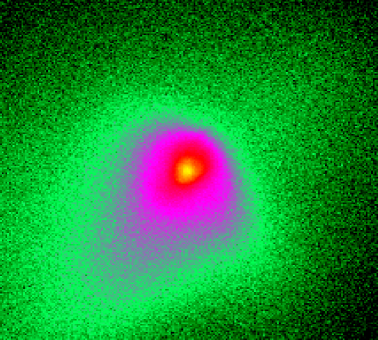
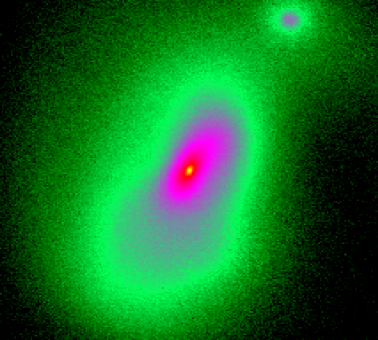
Figure 1: Collapse and fragmentation of a primordial cloud. We show the projected gas density at a redshift $z\simeq 21.5$, shortly after gravitational runaway collapse has converged at the center of the cloud. Left: The coarse-grained morphology in a box with a linear physical size of 23.5 pc. At this time, a gravitationally-bound clump has formed with a mass of $\sim 10^{3}M_{\odot}$. Right: The fine-grained morphology in a box with a linear physical size of 0.5 pc. The central density peak accretes mass vigorously, and is accompanied by a secondary clump.

Figure 2: Radial distribution of physical properties of SPH particles within the main clump. The presented snapshot was taken shortly before the central sink particle was created. (a) Hydrogen number density (in cm^-3) vs. radial distance from density maximum (in AU). For comparison, we also show the isothermal profile (dashed line), which provides a good description for the outer region. (b) Gas temperature (in K). (c) Radial velocity (in km s^-1). Dashed line: Radially averaged (negative) sound speed. It is evident that the flow is mostly subsonic, with a few fluid elements having mildly supersonic speeds. (d) Hydrogen molecule fraction. Within the central $\sim 100$ AU, three-body reactions have converted the gas into a fully molecular phase.

To study the formation of a Population III star, we have re-simulated the evolution of the central clump with sufficient resolution to follow its collapse up to a limiting density of $n\sim 10^{12}$ cm^-3, at which point opacity effects become important (see §2), and a sink particle is created. The right panel in Figure 1 shows the gas density on a scale of 0.5 pc. Several features are evident in this image. First, the central clump does not undergo further sub-fragmentation, and is likely to form a single Population III star. Second, a companion clump is visible at a distance of $\sim 0.25$ pc. If negative feedback from the first-forming star is ignored, this companion clump would undergo runaway collapse on its own, approximately $\sim 3$ Myr later. This timescale is comparable to the lifetime of a very massive star (e.g., Bromm et al., 2001). If the second clump were able to survive the intense radiative heating from its neighbor, it could become a star before the first one explodes as a SN. Whether more than one star can form in a low-mass halo thus crucially depends on the degree of synchronization of clump formation. Finally, the non-axisymmetric disturbance induced by the companion clump, as well as the angular momentum stored in the orbital motion of the binary system, allow the system to overcome the angular momentum barrier for the collapse of the central clump (see Larson, 2002), and to possibly form a wide binary star system.

In Figure 2, we consider the radial structure around the central density maximum, shortly before the accreting sink particle is created. The overall behavior is similar to previous results (Omukai and Nishi, 1998; Abel et al., 2002; Ripamonti et al., 2002). The density profile [panel (a)] consists of a central, flat core, surrounded by a roughly isothermal envelope. Such a configuration is generically predicted for collapsing star forming clumps (see Larson, 2003), and can approximately be described by the Larson-Penston similarity solution. Three-body reactions have succeeded in converting the central $\gtrsim 1M_{\odot}$ into fully molecular form [panel (d)]. Notice that the central temperature never drops precipitously due to the boost in H₂ cooling, even though H₂ is now more abundant by a factor of $\sim 10^{3}$. The opposite effects of compressional heating and H₂ formation heating balance the enhanced cooling rate, and lead to an almost isothermal collapse in the central region.

Next, we address the accretion flow onto the central sink particle by tracing its growth for $\sim 10^{4}$ yr after its initial formation. This accretion process will determine how massive the star finally gets. We begin with a brief discussion of the basic physics of the accretion, then describe the results from earlier 1D calculations, and finally compare these results to our simulation. In general, star formation typically proceeds from the ‘inside-out’ through the accretion of gas onto a central hydrostatic core (e.g., Larson, 2003). Even though the initial mass of the hydrostatic core in the Population III case is very similar to that in the Population I/II case, the accretion process is expected to be rather different. On dimensional grounds, the accretion rate simply scales as the sound speed cubed over Newton’s constant (or equivalently the ratio of the Jeans mass and the free-fall time): $\dot{M}_{\rm acc}\sim c_{s}^{3}/G\propto T^{3/2}$. A comparison of the temperatures in present-day star forming regions ($T\sim 10$ K) with those in primordial ones ($T\sim 200-300$ K) already indicates a difference in the accretion rate of more than two orders of magnitude.

Omukai and Palla (2001, 2003) extended earlier work by Stahler et al. (1986) and investigated the spherical accretion problem in considerable detail, going beyond the simple dimensional argument given above. Their computational technique approximates the time evolution by considering a sequence of steady-state accretion flows onto a growing hydrostatic core. Somewhat counterintuitively, these authors identified a critical accretion rate, $\dot{M}_{\rm crit}\sim 4\times 10^{-3}M_{\odot}$ yr^-1, beyond which the protostar cannot grow to masses much in excess of a few tens of solar masses. The critical rate is predicted to be almost independent of mass (Omukai and Palla, 2003). For smaller rates, however, the accretion is predicted to proceed all the way up to $\sim 600M_{\odot}$, i.e., of order the host clump mass. The physical origin of the critical accretion rate is that for ongoing accretion onto the core, the luminosity must not exceed the Eddington value, $L_{\rm EDD}$, if the inner region of the gaseous core is ionized by the central star. In our simulation, we do not resolve the evolution of the fully molecular core to temperatures and densities high enough to completely ionize the gas. Our estimate of the accretion rate, evaluated at the density where the gas becomes fully molecular, is likely to be applicable also at the higher density where the gas becomes fully ionized. This extrapolation assumes that the inflowing gas will not be diverted into outflows before reaching the central protostar. It will be important to test this assumption in future work, taking into account the magneto-hydrodynamics of possible bipolar jets. We now ask whether the growing star is able to settle onto the main sequence (MS), without experiencing a strong radiative feedback on the accretion flow. Before the onset of hydrogen burning, the luminosity is approximately given by $L_{\rm tot}\sim L_{\rm acc}\simeq GM_{\ast}\dot{M}_{\rm acc}/R_{\ast}$. Here, we have ignored the contribution to the overall luminosity from Kelvin-Helmholtz (KH) contraction for simplicity, as we are only aiming at an order-of-magnitude estimate. By setting $L_{\rm acc}\simeq L_{\rm EDD}$ it follows that

$$\dot{M}_{\rm crit}\simeq\frac{L_{\rm EDD}R_{\ast}}{GM_{\ast}}\sim 5\times 10^{-3}M_{\odot}{\rm~{}yr}^{-1}\mbox{\ ,}$$ (22)

where $R_{\ast}\sim 5R_{\odot}$, a typical value for a Population III MS star (e.g., Bromm et al., 2001). This is the critical accretion rate that must not be exceeded upon reaching the MS. If it is surpassed, radiation pressure on free electrons will drive a strong wind, thus preventing further accretion.

It is possible to start out with accretion rates that are significantly larger than $\dot{M}_{\rm crit}$, because at earlier times the protostellar radius is much larger, $R_{\ast}\gtrsim 100R_{\odot}$, and it only gradually shrinks to the MS value in the course of KH contraction. During the KH phase, the star is in hydrostatic equilibrium, but not yet in thermal equilibrium, which is only achieved on the MS when contraction temporarily stops. The above condition can only determine whether accretion is capable of incorporating most of the diffuse envelope into the star, or whether it is shut-off by radiation pressure early on. The precise stellar mass in the latter case can only be determined by a detailed simulation that takes both radiative-transfer and the hydrodynamics into account. Such a fully self-consistent calculation has not yet been achieved in three dimensions, although Omukai and Palla (2003), as well as Tan and McKee (2003), have treated this demanding problem in zero- and one dimension.

Realistic flows are expected to produce a time-dependent accretion rate, and so their outcome depends on whether the accretion rate declines rapidly enough to avoid exceeding the Eddington luminosity at some stage during the evolution. The main caveat concerning the Omukai and Palla (2001, 2003) results involves the geometry of the infall. A three-dimensional accretion flow of gas with angular momentum will deviate from spherical symmetry, and instead form a flattened rotating configuration such as a disk. In this case, most of the photons will likely escape along the rotation axis (where the gas density and the corresponding opacity is low) whereas mass may flow unimpeded along the disk plane (see Tan and McKee, 2003).

Figure 3: Accretion onto a primordial protostar. The morphology of the accretion flow is shown in Fig. 1. Left: Accretion rate (in $M_{\odot}$ yr^-1) vs. time (in yr) after the formation of a molecular core. Solid line: Accretion rates approximated as: $\dot{M}_{\rm acc}\propto t^{-0.25}$ for $t<10^{3}$ yr, and $\dot{M}_{\rm acc}\propto t^{-0.6}$ for $t>10^{3}$ yr. The early 3D evolution does not follow the simple power-law temporal behavior found in 1D simulations with very high resolution (Omukai and Nishi, 1998). Right: Mass of the central core (in $M_{\odot}$) vs. time. Solid lines: Accretion history approximated as: $M_{\ast}\propto t^{0.75}$ for $t<10^{3}$ yr, and $M_{\ast}\propto t^{0.4}$ for $t>10^{3}$ yr. Using this analytical approximation, we extrapolate that the protostellar mass grows to $\sim 120M_{\odot}$ after $\sim 10^{5}$ yr, and to $\sim 500M_{\odot}$ after $\sim 3\times 10^{6}$ yr, the lifetime of a very massive star.

In Figure 3, we show the accretion history. Our time-dependent, 3-dimensional simulation provides the accretion flow around a primordial protostar and shows how the molecular core grows in mass over the first $\sim 10^{4}$ yr after its formation. The accretion rate is initially very high, $\dot{M}_{\rm acc}\sim 0.1M_{\odot}$ yr^-1, and subsequently declines with time in a complex fashion. Expressed in terms of the sound speed in Population III pre-stellar cores, the initial rate is: $\dot{M}_{\rm acc}\sim 25c_{s}^{3}/G$. Initial accretion rates of a few tens times $c_{s}^{3}/G$ are commonly encountered in simulations of present-day star formation (Larson, 2003). We thus find that Population III stars reproduce this generic behavior. The mass of the molecular core, taken as an estimate for the protostellar mass, grows approximately as

$$M_{\ast}=\int\dot{M}_{\rm acc}{\rm d}t\approx 20M_{\odot}\left(\frac{t}{10^{3}\mbox{\ yr}}\right)^{0.75}$$ (23)

for $t<10^{3}$ yr, and as

$$M_{\ast}=\int\dot{M}_{\rm acc}{\rm d}t\approx 20M_{\odot}\left(\frac{t}{10^{3}\mbox{\ yr}}\right)^{0.4}$$ (24)

afterwards. The early-time accretion behavior is similar to the power-law scalings found in 1D, spherically symmetric simulations (Omukai and Nishi, 1998; Ripamonti et al., 2002). The complex accretion history encountered in our simulation, however, cannot be accommodated with a single power law. Such a multiple power-law behavior has previously been inferred (Abel et al., 2002; Omukai and Palla, 2003). This earlier inference, though, was indirect, in that it did not follow the actual accretion flow, but instead estimated the accretion from the instantaneous density and velocity profiles at the termination of the 3D simulation of Abel et al. (2002). Expressed as a function of stellar mass, our accretion rate scales as $\dot{M}_{\rm acc}\propto M_{\ast}^{-0.35}$ for $t<10^{3}$ yr, and $\dot{M}_{\rm acc}\propto M_{\ast}^{-1.5}$ afterwards. The early behavior is similar to the accretion law predicted by Tan and McKee (2003): $\dot{M}_{\rm acc}\propto M_{\ast}^{-0.4}$. In summary, our simulated accretion history at early times is consistent with previous estimates, based on 0D and 1D work, but deviates significantly at later times, at $t>10^{3}$ yr. Furthermore, the accretion flow is not a simple scale-free process when followed over a sufficiently long time. The self-similarity of the flow is broken because the presence of three-body reactions introduces a preferred timescale (see equ. (2)): $t_{\mbox{\scriptsize 3-body}}\sim 10^{3}$ yr.

Our simulations do not take into account any feedback effects from the proto-star on the accretion flow. To ascertain when these are likely to intervene, we compare our accretion history with the critical threshold derived by Omukai and Palla (2003). We find that as early as $\sim 3000$ yr after the accretion started, the accretion rate drops below $\dot{M}_{\rm crit}$, at which point the stellar mass is $M_{\ast}\sim 30M_{\odot}$. The accretion rate becomes sub-critical early on, while the protostar still undergoes KH contraction. Thus, according to the model of Omukai and Palla (2003), the star can settle onto the MS without experiencing a strong continuum-driven wind, and accretion can continue during the hydrogen-burning stage. A conservative upper limit for the final mass of the star is then, $M_{\ast}(t=3\times 10^{6}{\rm yr})\sim 500M_{\odot}$, assuming that accretion cannot go on for longer than the total lifetime of a very massive star, which is almost independent of stellar mass (e.g., Bond et al., 1984; Bromm et al., 2001).

5 Conclusions

We have presented the first three-dimensional simulation of Population III star formation that followed the accretion flow for $\sim 10^{4}$ yr, allowing to better estimate the final stellar mass. The earlier collapse phase prior to the formation of the initial hydrostatic core, gives results that are similar to previous work (Omukai and Nishi, 1998; Abel et al., 2002; Ripamonti et al., 2002). In particular, we confirm that the gas is converted into a fully molecular phase due to three-body reactions within the central $\sim 100$ AU (comprising an initial mass of $\gtrsim 1M_{\odot}$). When extrapolating the accretion to $\sim 3\times 10^{6}$ yr, the lifetime of a massive star, we get $M_{\ast}\sim 500M_{\odot}$.

Can a Population III star ever reach this asymptotic mass limit? Our hydrodynamic simulation lacks radiative transfer and cannot address this question, as the answer depends on whether the accretion from the dust-free envelope is eventually terminated by feedback from the star (e.g., Omukai and Palla, 2001, 2003; Ripamonti et al., 2002; Omukai and Inutsuka, 2002; Tan and McKee, 2003). The standard mechanism by which accretion may be terminated in metal-rich gas, namely radiation pressure on dust grains (Wolfire and Cassinelli, 1987), is obviously not effective for gas with a primordial composition. It has been speculated that accretion could instead be turned off through the formation of an H II region (Omukai and Inutsuka, 2002), or through the radiation pressure exerted by trapped Ly$\alpha$ photons (Tan and McKee, 2003). The unsolved problem of whether the accretion process is terminated by radiative feedback from the protostar, defines the current frontier in three-dimensional numerical studies of the formation of Population III stars.

Acknowledgements

We thank an anonymous referee for constructive comments that helped improve the paper. This work was supported in part by NASA grant NAG 5-13292, and by NSF grants AST-0071019, AST-0204514.

References

- \harvarditemAbel, Bryan, Norman2002abn02 Abel, T., Bryan, G., Norman, M. L., 2002. Science 295, 93.
- [1] \harvarditemBarkana, Loeb2001bl01 Barkana, R., Loeb, A., 2001. Phys. Rep. 349, 125.
- [2] \harvarditemBBB2003bbb03 Bate, M. R., Bonnell, I. A., Bromm, V., 2003. MNRAS 339, 577.
- [3] \harvarditem1984bac99 Bond, J. R., Arnett, W. D., Carr, B. J., 1984. ApJ 280, 825.
- [4] \harvarditemBromm2000b00 Bromm, V., 2000. Star Formation in the Early Universe. PhD Thesis. Yale Univ., New Haven.
- [5] \harvarditem2004Br04 Bromm V., 2004. PASP, in press (astro-ph/0311292).
- [6] \harvarditemBromm, Coppi, Larson1999bcl99 Bromm, V., Coppi, P. S., Larson, R. B., 1999. ApJ 527, L5.
- [7] \harvarditemBromm, Coppi, Larson2002bcl02 Bromm, V., Coppi, P. S., Larson, R. B., 2002. ApJ 564, 23.
- [8] \harvarditemBromm, Kudritzki, Loeb2001bkl Bromm, V., Kudritzki, R. P., Loeb, A., 2001. ApJ 552, 464.
- [9] \harvarditemBromm, Loeb2003bl03 Bromm, V., Loeb, A., 2003. ApJ 596, 34.
- [10] \harvarditem2003byh03 Bromm, V., Yoshida, N., Hernquist, L., 2003. ApJ 596, L135.
- [11] \harvarditemCen2003cen03 Cen, R., 2003. ApJ 591, L5.
- [12] \harvarditemCiardi, Ferrara, White2003cfw03 Ciardi, B., Ferrara, A., White, S. D. M., 2003. MNRAS 344, L7.
- [13] \harvarditem2003fl03 Furlanetto, S. R., Loeb, A., 2003. ApJ 588, 18.
- [14] \harvarditem2003hh03 Haiman, Z., Holder, G. P., 2003. ApJ 595, 1.
- [15] \harvarditem2002hw02 Heger, A., Woosley, S. E., 2002. ApJ 567, 532.
- [16] \harvarditem1989hk89 Hernquist, L., Katz, N., 1989. ApJS 70, 419.
- [17] \harvarditem1979hm79 Hollenbach, D., McKee, C. F., 1979. ApJS 41, 555.
- [18] \harvarditem2001jh01 Jang-Condell, H., Hernquist, L., 2001. ApJ 548, 68.
- [19] \harvarditem2003kap03 Kaplinghat, M., Chu, M., Haiman, Z., Holder, G. P., Knox, L., Skordis, C., 2003. ApJ 583, 24.
- [20] \harvarditem1991katz91 Katz, N., 1991. ApJ 368, 325.
- [21] \harvarditem1991katz91 Kitsionas, S., Whitworth, A. P., 2002. MNRAS 330, 129.
- [22] \harvarditem2003kog03 Kogut, A., et al., 2003. ApJS 148, 161.
- [23] \harvarditemLars1969l69 Larson, R. B., 1969. MNRAS 145, 271.
- [24] \harvarditemLars2002l02 Larson, R. B., 2002. MNRAS 332, 155.
- [25] \harvarditemLars2003l03 Larson, R. B., 2003. Rep. Prog. Phys. 66, 1651.
- [26] \harvarditem2003mbh03 Mackey, J., Bromm, V., Hernquist, L., 2003. ApJ 586, 1.
- [27] \harvarditem2001mfr01 Madau, P., Ferrara, A., Rees, J. M., 2001. ApJ 555, 92.
- [28] \harvarditem2002mfm02 Mori, M., Ferrara, A., Madau, P., 2002. ApJ 571, 40.
- [29] \harvarditem2001nu01 Nakamura, F., Umemura, M., 2001. ApJ 548, 19.
- [30] \harvarditemNorman et al.2003no03 Norman, M. L., O’Shea, B.W., Paschos P., 2004. ApJL, in press (astro-ph/0310758).
- [31] \harvarditem2002oi02 Omukai, K., Inutsuka, S., 2002. MNRAS 332, 59.
- [32] \harvarditemOmukai and Nishi1998on98 Omukai, K., Nishi, R., 1998. ApJ 508, 141.
- [33] \harvarditemOmukai and Palla2001op01 Omukai, K., Palla, F., 2001. ApJ 561, L55.
- [34] \harvarditemOmukai, Palla2003op03 Omukai, K., Palla, F., 2003. ApJ 589, 677.
- [35] \harvarditem1993pad93 Padmanabhan, T., 1993. Structure Formation in the Universe. Cambridge Univ. Press, Cambridge.
- [36] \harvarditem1983pss83 Palla, F., Salpeter, E. E., Stahler, S. W., 1983. ApJ 271, 632.
- [37] \harvarditemRipamonti et al.2002rip02 Ripamonti, E., Haardt, F., Ferrara, A., Colpi, M., 2002. MNRAS 334, 401.
- [38] \harvarditem1979rl79 Rybicki, G. B., Lightman, A. P., 1979. Radiative Processes in Astrophysics. Wiley, New York.
- [39] \harvarditemScannapieco et al.2003sc03 Scannapieco, E., Schneider, R., Ferrara, A., 2003. ApJ 589, 35.
- [40] \harvarditem2002sch02 Schaerer, D., 2002. A&A 382, 28.
- [41] \harvarditem2002sch02 Schneider, R., Ferrara, A., Natarajan, P., Omukai, K., 2002, ApJ 571, 30.
- [42] \harvarditem1991shu91 Shu, F. H., 1991. The Physics of Astrophysics. I. Radiation. Univ. Science Books, Mill Valley.
- [43] \harvarditem2003sok03 Sokasian, A., Yoshida, N., Abel, T., Hernquist, L., Springel, V., 2003. MNRAS, submitted (astro-ph/0307451)
- [44] \harvarditem2003sl03 Somerville, R. S., Livio, M., 2003. ApJ 593, 611.
- [45] \harvarditem2003spe03 Spergel, D. N., et al., 2003. ApJS 148, 175.
- [46] \harvarditem1986sps86 Stahler, S. W., Palla, F., Salpeter, E. E., 1986. ApJ 302, 590.
- [47] \harvarditemTan, McKee2003tan03 Tan, J. C., McKee, C.F. 2003, ApJ, in press (astro-ph/0307414).
- [48] \harvarditem1997teg97 Tegmark, M., Silk, J., Rees, M. J., Blanchard, A., Abel, T., Palla, F., 1997. ApJ 474, 1.
- [49] \harvarditem1998tru98 Truelove, J. K., Klein, R. I., McKee, C. F., Holliman, J. H., Howell, L. H., Greenough, J. A., Woods, D. T., 1998. ApJ 495, 821.
- [50] \harvarditemTumlinson and Shull2000tum00 Tumlinson, J., Shull, J. M., 2000. ApJ 528, L65.
- [51] \harvarditem1977tkd77 Turner, J., Kirby-Docken, K., Dalgarno, A., 1977. ApJS 35, 281.
- [52] \harvarditem2002un02 Umeda, H., Nomoto, K., 2002. ApJ 565, 385.
- [53] \harvarditem2003un03 Umeda, H., Nomoto, K., 2003. Nature 422, 871.
- [54] \harvarditemWV2003wv03 Wada, K., Venkatesan, A., 2003. ApJ 591, 38.
- [55] \harvarditem1987wc87 Wolfire, M. G., Cassinelli, J. P., 1987. ApJ 319, 850.
- [56] \harvarditemWyithe, Loeb2003wl03 Wyithe, J. S. B., Loeb, A., 2003. ApJ 588, L69.
- [57] \harvarditem2003yosh03 Yoshida, N., Abel, T., Hernquist, L., Sugiyama, N., 2003. ApJ 592, 645.
- [58] \harvarditem2004ybh03 Yoshida, N., Bromm, V., Hernquist, L., 2004. ApJ, submitted (astro-ph/0310443)
- [59] \harvarditem1970zeld70 Zeldovich, Y. B., 1970. A&A 5, 84.
- [60]