Constraining the reionization history with large angle CMB polarization

Abstract

The first-year WMAP data release showed that the reionization optical depth to CMB photons is greater than previously thought. This follows from unexpectedly high values of the $C^{TE}_{l}$ spectrum, for $l$ up to $\sim 30$, presumably allowing a measurement of the E-mode polarization spectrum $C^{E}_{l}$, sooner than expected. This note aims to test the capability of large-angle polarization experiments to explore the history of the cosmological reionization, considering also the impact of cosmic variance. In particular, here we discuss how well the ionized fraction $x_{e}$ and the reionization redshift $z_{r}$ can be separately measured, at various levels of instrumental noise.

1 Introduction

In the last ten years, measures on Cosmic Microwave Background (CMB) have reached high sensitivity and resolution (see, e.g., [1, 2, 3, 4, 5]), providing the spectrum of temperature anisotropies, $C_{l}^{T}$, up to $l\sim 1000$. This allowed to better constrain various parameters of the cosmological model. Among them, the optical depth $\tau$, due to reionization, has a peculiar character. Other parameters directly reflect initial conditions and/or inflationary outputs; the value of $\tau$, instead, conveys information on the physical conditions in the Universe due to more recent events, and opens an observational window on the physics of ancient cosmic objects. Furthermore, while other parameters influence data through linear physics, the cosmic opacity $\tau$ is clearly linked to later non–linear evolution.

Unfortunately, $\tau$ is only mildly constrained by $C_{l}^{T}$, because of a degeneracy with the primordial spectral index ($n$) of density fluctuations ([6, 7]; see also [8]). For this reason, pre–WMAP $C_{l}^{T}$ data could only constrain $\tau$ to be $\mathrel{\mathchoice{\vbox{\offinterlineskip\halign{\hfil$\displaystyle#$\hfil\cr<\cr\sim\cr}}}{\vbox{\offinterlineskip\halign{\hfil$\textstyle#$\hfil\cr<\cr\sim\cr}}}{\vbox{\offinterlineskip\halign{\hfil$\scriptstyle#$\hfil\cr<\cr\sim\cr}}}{\vbox{\offinterlineskip\halign{\hfil$\scriptscriptstyle#$\hfil\cr<\cr\sim\cr}}}}0.40$, at the 2–$\sigma$ level [9]. On the other hand, several models of reionization hinted at a value of the optical depth in the range $0.03-0.05$ (see, e.g, [10]).

The recent WMAP first–year release has significantly modified the context, thanks to data on the $ET$–correlation spectrum, $C_{l}^{ET}$. Quite in general, $C_{l}^{ET}$ and the $E$–polarization spectrum $C_{l}^{E}$ contain independent information on $\tau$. In particular, the most part of this information is conveyed by the spectral components with $l\mathrel{\mathchoice{\vbox{\offinterlineskip\halign{\hfil$\displaystyle#$\hfil\cr<\cr\sim\cr}}}{\vbox{\offinterlineskip\halign{\hfil$\textstyle#$\hfil\cr<\cr\sim\cr}}}{\vbox{\offinterlineskip\halign{\hfil$\scriptstyle#$\hfil\cr<\cr\sim\cr}}}{\vbox{\offinterlineskip\halign{\hfil$\scriptscriptstyle#$\hfil\cr<\cr\sim\cr}}}}30$; it is their unexpectedly high amplitude that led to estimate $\tau\simeq 0.17\pm 0.04$ [11].

In the presence of such signal, it is legitimate to wonder whether current (or more advanced) experiments can succeed in providing us with more information on reionization, besides the value of $\tau$. In this work we shall refer to the expected performance of the Sky Polarization Observatory (SPOrt [12, 13, 14]), first to outline its capacity to provide an independent confirm of the high $\tau$ value, by using high–sensitivity polarimeters operating at three MW frequencies (22, 32 and 90 GHz). Then, we shall focus on the capability of low–$l$ polarization experiments to inspect the cosmic reionization history, by analyzing the expected outputs of experiments run at increasing levels of sensitivity. Our conclusions directly apply to any (nearly–)full sky experiment with a design similar to SPOrt; using them for possible future experiment, with minor technical differences, is substantially harmless.

At large angular scales, cosmic variance (CV) can never be neglected and risks to reduce the strength of CMB data in constraining the reionization history. One of the main difficulties of this analysis amounts to taking carefully into account its effects. We shall see that, as these effects interfere with low–$l$ inspections, a sensitivity much higher than the one of WMAP or SPOrt ought to be reached, before the full potentiality of large angles results is exploited.

2 Monte Carlo analysis

2.1 Model properties

An optical depth $\tau=0.17\pm 0.04$ corresponds to a reionization redshift $z_{r}\simeq 17\pm 5$, assuming a sharp reionization in a $\Lambda$CDM model with WMAP best fit parameters. On the other hand, the Gunn–Peterson effect seems to affect high-$z$ quasar radiation ([15, 16]), emitted at redshift $\simeq 6$; this shows that at least a fraction (possibly as small as $1\,\%$) of neutral hydrogen was still present at that time. Taken together, these observations imply that reionization is a fairly complex process, and that its complete characterization requires more than the value of the optical depth ([17]).

To account for such an observational picture, several models have been proposed, including double reionization models ([18, 19]) or a period of extended reionization ([20]), but more complex pictures are possible. A feature common to most these models is a bump in $C_{l}^{E}$ and $C_{l}^{TE}$ spectra at low $l$, but other effects can be expected, involving spectral components up to $l>1000$. The analysis carried on in this work is based on a partial reionization model, in which baryonic materials reionize abruptly at a redshift $z_{r}$, attaining a reionization fraction $x_{e}\leq 1$. Thus, a given value of $\tau$ corresponds to different $x_{e}-z_{r}$ pairs. Although this is admittedly a toy model, it may reasonably approximate a large family of possible reionization histories. We shall take other relevant cosmological parameters as known from independent data (e.g., from high–$l$ spectral analysis); we fix their values as follows: a flat spatial section with reduced density parameters $\Omega_{m}h^{2}=0.147$, $\Omega_{b}h^{2}=0.024$ (for matter and baryons, respectively), the Hubble parameter is 70 km/s/Mpc and the primeval spectral index is $n=1$. We assume no contributions from tensor modes of gravity perturbation; this means, in particular, no $B$-mode polarization. In a previous work ([8]) we tested that, in practice, likelihood results are insensitive to reasonable variations of these parameters.

Parameter estimation from CMB data usually follows a Bayesian maximum likelihood approach (see, e.g., [21, 22]). In this work, however, we are mainly interested in polarization measures at large angles, to test how they can improve the reconstruction of the reionization history. Therefore, we adopted a Monte Carlo approach to directly account for CV, and performed a wide set of realizations of four models, corresponding to $\tau=0.17$ or 0.13 with $x_{e}$ = 0.6 or 1.

Artificial anisotropy and polarization data were built using CMBFAST and HEALPix codes. The resulting maps have been smoothed with a purely Gaussian filter of $7^{o}$ FWHM, to represent SPOrt instruments beam, and we chose a HEALPix resolution $N_{side}=16$, corresponding to a pixels’ width of $\simeq 3.5^{o}$, thus approaching the Nyquist frequency of the configuration. At the angular scales considered here, the non-ideality of SPOrt’s feed horns give rise to a spurious polarization signal due mainly to the temperature anisotropy signal smoothed on scales equal to the instruments’ FWHM. Assuming a rms $T$ intensity of $\sim 30\mu$K, this translates into a rms contamination $<0.2\mu$K, which is roughly an order of magnitude smaller than the expected noise of the SPOrt experiment [12, 23].

We considered increasing levels of sensitivity for polarization (noise-per-pixel $\sigma_{pix}=2$, 1, 0.5, 0.1$\,\mu$K). The first value should be achieved by combining the two 90 GHz SPOrt-channels, after two years of data taking, while using the 22 and 32 GHz channels to map and remove the galactic foregrounds contamination. Temperature noise was held fixed to $\sigma^{T}_{pix}=1\mu$K, roughly the value expected for the 4-year WMAP results. As on large scales signal-to-noise ratio in temperature signal is much more than unity, varying temperature noise in the same range of $\sigma_{pix}$ does not affect our results. Noise was assumed to be uncorrelated, both between different pixels and between the different Stokes parameters. For each choiche of $\tau$, $x_{e}$ and $\sigma_{pix}$, 1000 independent sets of artificial data were considered.

2.2 Likelihood evaluation

When multi-parameter analysis for small angle experiments is required, likelihood computation rapidly becomes time intensive, forcing the adoption of various approximations (see, e.g., [22, 24]) or even a fisher-matrix approach. In this work, however, we are interested mainly in how polarization measures at large angles can improve the reconstruction of the reionization history. Moreover, SPOrt large beam size implies that data will be binned to a fairly low number of pixels. Together, these considerations make the evaluation of the full likelihood function in coordinate, or pixel, space feasible for a reduced number of parameters. This has the added advantage of simplifying the joint likelihood between experiments with different sky coverages.

An artificial CMB sky map is a realization of a given cosmological model $\cal M$ whose statistical properties (i.e. the sets of $C^{Y}_{l}$ coefficients, with $Y=T,E,TE$) are known. On each pixel, measures of temperature fluctuations ($T$) and of the $Q$ and $U$ Stokes parameters are ideally performed.

Galactic foregrounds contamination is a serious issue in $T$ maps, we therefore exclude the Galactic plane (i.e. the region of sky with Galactic declination $|\delta_{g}|<20^{o}$) from anisotropy maps. In the case of polarization, Galactic contamination, while still an issue, plays a less important role. The first year WMAP data showed that the most prominent foreground contribution is due to Galactic synchrotron, whose polarization spectrum has a steep dependency on frequency. According to the synchrotron template developed by the SPOrt team[25], at 90-100 GHz CMB polarization should dominate over foregrounds contamination by a factor of 2-3 to almost 1 order of magnitude, depending on the value of the optical depth. Accordingly, we exclude from polarization maps only the equatorial polar caps, with declination $|\delta|>51.6^{o}$, which SPOrt will not be able to inspect from its position on board the ISS. Notice that the polar caps partly overlap with the Galactic plane. The number of pixels available for anisotropy (polarization) measures is therefore $N_{T}=1984$ ($N_{P}=2404$). These data form a $(N_{T}+2N_{P})$-components vector ${\bf x}\equiv\{T(i=1,...,N_{T}),Q(i=1,....,N_{P}),U(i=1,....,N_{P})\}$.

The statistical properties of the process underlining the synthetic data vector can be expressed through the correlation matrix $\langle{\bf x^{T}}_{i}{\bf x}_{j}\rangle\equiv{\bf C}_{ij}={\bf S}_{ij}+{\bf N}_{ij}$, where the brackets mean ensemble average. In particular, the correlation matrix has been written as the sum of a signal term ${\bf S}_{ij}$, which depends on cosmology and geometry, and a term which accounts for detector noise.

The expected anisotropy correlation between two pixels with angular separation $\vartheta_{ij}$ is given by

$$\langle T_{i}T_{j}\rangle=\sum_{l}{2l+1\over 4\pi}C^{T}_{l}P_{l}(\cos\vartheta_{ij})B^{2}_{l};$$ (1)

where $P_{l}(\cos\vartheta_{ij})$ are Legendre polynomials and $B^{2}_{l}$ are reduction coefficients due to pixelization and beam smoothing. For other correlations, similar expressions hold and can be evaluated using the relations given in [21].

We assume no correlation among noise in different modes and pixels, so $\bf N$_ij is diagonal and has distinct values $(\sigma^{T}_{pix})^{2}$ and $\sigma_{pix}^{2}$ in the former $N_{T}$ and in the latter $2N_{P}$ pixels, respectively.

Assuming Gaussian statistics, the likelihood of a model $\cal M^{\prime}$ given the synthetic data x reads then:

$${\cal L}({\cal M^{\prime}}|{\bf x})={1\over(2\pi)^{N_{T}+2N_{P}}}{1\over\sqrt{\det{\bf C^{\prime}}}}\exp\left(-{1\over 2}{\bf x}^{\rm T}{\bf C^{\prime}}^{-1}{\bf x}\right)~{}.$$ (2)

In a Bayesian analysis, the posterior probability density is given by the product of the likelihood function and the prior probability density. According to Bayes theorem, in the case of an uniform prior the most likely model is the one for whom the likelihood function is maximum. Confidence regions in parameter space are then found by a likelihood ratio criterion. These regions are also called credibility regions and generally represent only an approximation to the true confidence intervals, particularly when CV is significant.

A frequentist analysis, instead, stems from the question: What is the probability of obtaining a given output from an observation if the underlying physical process has a certain set of parameters? To answer this question, the usual procedure is to generate a large set of synthetic observations, analyze them as real data, and then study the distribution of the results. Confidence regions, which in this case are exclusion regions, are determined as the portion of parameter space which contain a set percentage of the total results.

3 Results

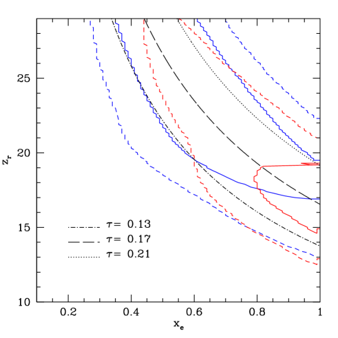
Figure 1: Expected likelihood contours in the $x_{e}-z_{r}$ plane for models with $\tau=0.17$ and two different reionization histories; $\sigma_{pix}=2\mu$K. Solid and short-dashed lines trace the boundary of the 68% and 95% confidence level regions, respectively. In red we plot results for a model in which reionization is complete, while blue lines refer to a model in which $x_{e}=0.6$. Likelihood contours are elongated along direction of constant optical depth end do not allow to distinguish between the two models.

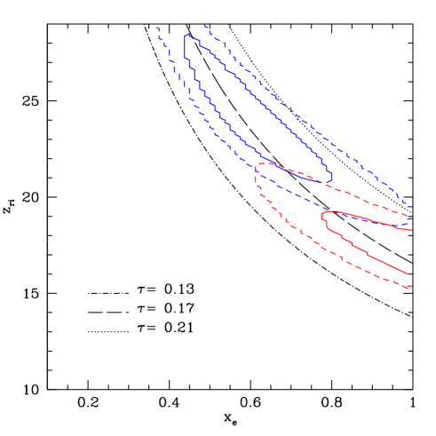
Figure 2: Same as figure 1, but with $\sigma_{pix}=0.5\mu$K. Likelihood function are elongated along lines of constant $\tau$, it is possible to distinguish between the two models at least at 68% c.l.

For each simulated sky, likelihood distributions have been evaluated on the $x_{e}$-$z_{r}$ plane. We show results in two ways: first, we average over the whole set of 1000 realizations and show 1 and 2–$\sigma$ confidence regions (see figure 1 and figure 2). Outside of them, we have exclusion regions, i.e. the portions of the $x_{e}$-$z_{r}$ that can be excluded with a given degree of confidence, taking into account the variance both in the detector noise and in the true CMB data. For the range of $\sigma_{pix}$ we tested, with the exception of the lowest value, the detector noise variance however dominates polarization measures, while the proper CV is more relevant for anisotropy data, where the signal to noise ratio is higher.

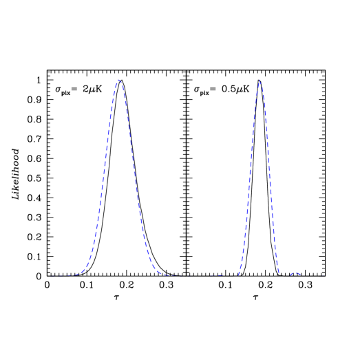
Figure 3: Likelihood function after marginalizing over $x_{e}$, for the models of figure 1. Results are plotted as a function of $\tau$ instead of $z_{r}$. Solid lines refer to complete reionization, dashed lines to $x_{e}=0.6$. No significant bias in the determination of the optical depth is introduced by the reionization histories considered here.

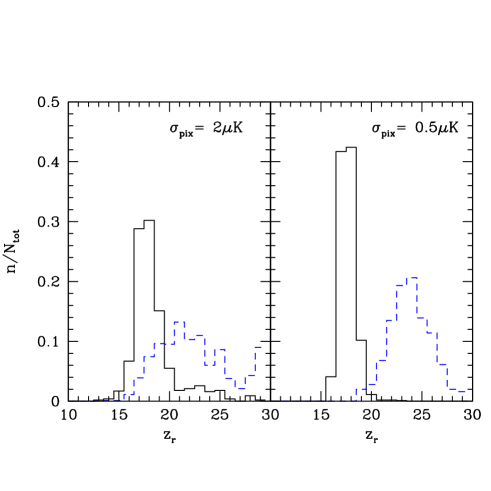
Figure 4: Histogram of the distribution of the maximum likelihood value of $z_{r}$, for models with $\tau=0.17$ and different reionization histories. Solid lines refer to $x_{e}=1,\,z_{r}\simeq 17$, dashed lines to $x_{e}=0.6,\,z_{r}\simeq 24$. Neat separation of the two distributions requires pixel noises $\sim 0.5\mu$K.

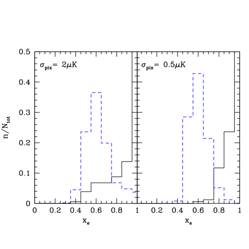
Figure 5: Same as figure 4, but for $x_{e}$.

However, when CV is significant, as it is for the angular separations considered here, the statistical properties of a realization can differ significantly from those of the underlying process. It is therefore significant to show how maximum likelihoods parameters are distributed. In figure 3, the distribution on $\tau$ is shown, both for $\sigma_{pix}=2$ and 0.5$\,\mu$K; solid (dashed) lines refer to the case $x_{e}=1~{}~{}(=0.6)$. This plot is meant to test how far $\tau$ determinations are affected by the actual reionization history. Then, in figure 4, we report the maximum likelihood distribution over $x_{e}$, after marginalizing over $z_{r}$. Finally, in figure 5, the distribution over $x_{e}$ is shown, after marginalizing over $z_{r}$. The same values of $\sigma_{pix}$ are considered, while solid and dashed lines refer to the same cases as above.

4 Discussion

Figure 1 shows the 1 and 2–$\sigma$ confidence regions for models with $\tau=0.17$, when $\sigma_{P}=2\mu$K. They clearly show a likelihood distribution elongated along the constant optical depth directions; this confirms that CMB data, for current noise levels, can provide constraints only on the integrated value $\tau$ (see, e.g. [26],[27]), but also that such constraints are fairly safe.

Figure 2 shows the 1 and 2–$\sigma$ confidence regions, still for models with $\tau=0.17$, but when $\sigma_{pix}=0.5\mu$K. At this pixel noise level, the polarization sensitivity allows us to constrain an additional parameter ($x_{e}$ or $z_{r}$) beside $\tau$, at least with a 68% c.l. Once again, by marginalizing, e.g., over $x_{e}$, we obtain the behaviour of the likelihood as a function of $\tau$. Figure 3 confirms that determination of the optical depth is substantially independent from the reionization history, at least within the range of reionization models considered here (however, other reionization histories can bias $\tau$ determinations [28]). This is true both for $\sigma_{pix}=2$ and 0.5$\,\mu$K.

By inspecting figure 4, we notice that, for the noise levels currently achievable ($\sigma_{pix}\simeq 2\,\mu$K), the distributions of maximum likelihood values are greatly superimposed and it is not possible to distinguish between the two reionization histories. On the contrary, for $\sigma_{pix}=0.5\,\mu$K, the superposition is restricted to the extreme tails of histograms; accordingly, at such a noise level, some details on the reionization history can be inspected. Notice that these plots provide the probability at which a given model can be excluded by the available data, instead of telling us the likelihood of a given model being the correct one, as is instead done in Bayesian analysis.

For both sensitivities, however, the distribution corresponding to $x_{e}=1$ is more sharply defined than the one corresponding to $x_{e}=0.6$. This is due to the fact that in the former case the true model necessarily lies on the boundary of the portion of parameter space considered. Analogous considerations could be made if, instead of marginalizing on the reionization fraction, we had marginalized over $z_{r}$, as it is shown in figure 5.

As outlined above, in this work we inspected a number of further cases, for which no plot is given. In particular, models with $\tau=0.13$ show quite a similar behavior, although some difference, on the level of noise required to achieve a clean separation of the two models, exists. In particular, the overlap between maximum likelihood histograms, for $\sigma_{pix}=0.5~{}\mu$K worsens from 2$\%$ to $4.5\,\%$. For all cases, considering $\sigma_{pix}=1\,\mu$K yields intermediate results.

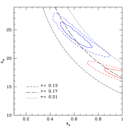
Figure 6: Same as figure 1, but with $\sigma_{pix}=0.1\mu$K. Clean separation between the two models is achieved at better than 95% c.l.

We report here also results obtained for $\sigma_{pix}=0.1\,\mu$K. While this noise level is certainly beyond the capabilities of current instruments, it should be achieved by the PLANCK experiment. While much of the information on reionization histories considered here is carried by the low-multipoles, PLANCK’s higher spatial and frequency resolutions provide an advantage in the form of reduced sidelobes contamination and a better monitoring of foregrounds. Simulations show that clean separation between the two different reionization histories should be achieved at more than 95% c.l., even taking into account CV (see figure 6). Moreover, at these noise levels, contribution from $B$-mode polarization should no longer be ignored, and could provide additional constraints on reionization. These, too, should be detected by the PLANCK satellite.

5 Conclusions

After the WMAP first-year results, it has become clear that reionization history is a complex process and CMB measures can provide unique information about it. In particular, CMB polarization (and, to a lesser extent, temperature-polarization cross correlations) encode a great deal of information not only on the total optical depth, but also on the evolution with time of the ionized fraction. However, this knowledge is found mainly in the first $l\mathrel{\mathchoice{\vbox{\offinterlineskip\halign{\hfil$\displaystyle#$\hfil\cr<\cr\sim\cr}}}{\vbox{\offinterlineskip\halign{\hfil$\textstyle#$\hfil\cr<\cr\sim\cr}}}{\vbox{\offinterlineskip\halign{\hfil$\scriptstyle#$\hfil\cr<\cr\sim\cr}}}{\vbox{\offinterlineskip\halign{\hfil$\scriptscriptstyle#$\hfil\cr<\cr\sim\cr}}}}30$ multipoles, i.e. at large angles. These scales are strongly affected by cosmic variance; therefore, the statistical properties of the actual sky can differ significantly from those of the underlying cosmological model.

In this work we investigated whether measures of CMB power spectra at large angular separations can provide actual constraints on reionization history. In particular, we considered the SPOrt project as a benchmark of a large angles polarization measurements, though we also explored instrumental sensitivities better than those of the actual experiment. We considered toy models with the same optical depth, but different fractions of ionized baryons; in both case we assumed an instantaneous reionization.

Using a frequentist analysis, we confirmed that, at the noise levels currently achievable, CMB data can provide informations mainly on the total optical depth. The SPOrt experiment will therefore provide the first independent confirmation of WMAP results on the optical depth, in a manner completely free of any spurious leakage between the $T$ and $E$ signals.

Distinguishing between a model in which all baryons reionized from a model in which the ionized fraction reaches only 60% requires, instead, noise levels significantly lower. In particular we found that, for $\tau=0.17$, discriminating between the two models at 68% c.l. requires a polarization pixel noise $\sigma_{pix}=0.5\mu$K, while for $\mathrel{\mathchoice{\vbox{\offinterlineskip\halign{\hfil$\displaystyle#$\hfil\cr>\cr\sim\cr}}}{\vbox{\offinterlineskip\halign{\hfil$\textstyle#$\hfil\cr>\cr\sim\cr}}}{\vbox{\offinterlineskip\halign{\hfil$\scriptstyle#$\hfil\cr>\cr\sim\cr}}}{\vbox{\offinterlineskip\halign{\hfil$\scriptscriptstyle#$\hfil\cr>\cr\sim\cr}}}}95\%$ c.l. $\sigma_{pix}\sim 0.1\,\mu$K is needed. While the models of reionization considered here are admittedly simplified, they provide two extreme examples of behaviour while being consistent with the currently available data. Moreover, our main aim was the determination of the sensitivity needed to extract information on an additional reionization parameter from CMB data. A complete assessment of the effects of a generic reionization history on CMB power spectra is certainly beyond the scope of this note, as it requires a completely different approach. In particular the non-uniform, or patchy, nature of the reionization process should be considered. This usually implies additional features at multipoles $l\mathrel{\mathchoice{\vbox{\offinterlineskip\halign{\hfil$\displaystyle#$\hfil\cr>\cr\sim\cr}}}{\vbox{\offinterlineskip\halign{\hfil$\textstyle#$\hfil\cr>\cr\sim\cr}}}{\vbox{\offinterlineskip\halign{\hfil$\scriptstyle#$\hfil\cr>\cr\sim\cr}}}{\vbox{\offinterlineskip\halign{\hfil$\scriptscriptstyle#$\hfil\cr>\cr\sim\cr}}}}1000$, which need to be inspected in order to fully exploit the information on reionization encoded in CMB.

Nonetheless, our results confirm that large angles polarization data can be used to discriminate between different reionization histories, but that next generation CMB (polarization) experiments will be indispensable for shedding light on those details of the reionization process that can be inspected through this observational window.

References

References

- [1] Smoot G, et al, 1992 ApJ 396 L1
- [2] de Bernardis P, et al, 2000 Nature 404 955
- [3] Hanany S, et al, 2000 ApJ L5
- [4] Halverson N W, et al, 2002 ApJ 568 38
- [5] Bennet C L, et al, 2003 ApJ Submitted.
- [6] Jungman G, Kamionkowski M, Kosowsky A and Spergel D N, 1996 Phys Rev D 54 1332
- [7] Eisenstein J E, Hu W and Tegmark M, 1998 ApJ 518 2
- [8] Colombo L P L and Bonometto S A, 2003 New Ast 8 313
- [9] Stompor R et al, 2001 ApJ 561 L7
- [10] Miralda-Escudé J, 2002 ApJ submitted [astro-ph/0211071]
- [11] Kogut A et al, 2003 ApJ submitted [astro-ph/0302213]
- [12] Cortiglioni S et al, 2003 NewA in press
- [13] Carretti E et al, 2000, in IAU Symposium 201, New Cosmological Data and the Value of Fundamental Parameters eds. Lasenby A and Wilkinson A, Astron. Soc. Pacif. Conf. Series
- [14] Macculi C et al, 2000 in What are the Prospect for Cosmic Physics in Italy? eds. Aiello S and Blanco A, Conf. Proc. 68, 171
- [15] Djorgovski S G, Castro S M, Stern D and Mahabal A A, 2001 ApJ 560 L5
- [16] Becker R H et al, 2001 AJ 122 6
- [17] Ciardi B, Ferrara A and White S D M, 2003 MNRAS submitted [astro-ph/0302451]
- [18] Cen R, 2003 ApJ in press [astro-ph/0210473]
- [19] Wythe J S B and Loeb A, 2003 ApJ 586 693
- [20] Haiman Z and Holder G, 2003 ApJ submitted [astro-ph/0302403]
- [21] Zaldarriaga M, 1998 ApJ 503 1
- [22] Verde L et al, 2003 ApJ submitted [astro-ph/0302218]
- [23] Carretti E et al, 2001 NewA 6 173
- [24] Bond J R, Jaffe A H and Knox L, 2000 ApJ 533 19
- [25] Bernardi G et al, 2003 MNRAS 344 347
- [26] Bruscoli M, Ferrara A and Scannapieco E, 2002 MNRAS 330 L43
- [27] Kaplinghat M et al, 2003 ApJ 583 24
- [28] Holder G, Haiman Z, Kaplinghat M and Knox L, 2003 ApJ submitted [astro-ph/0302404]
- [29] Venkatesan A, 2002 ApJ 572 15
- [30] Gorski K M, Hivon E and Wandelt B D, 1999 in Proceedings of the MPA/ESO Cosmology Conference ”Evolution of Large-Scale Structure”, eds. Banday A J, Sheth R S and Da Costa L, PrintPartners Ipskamp, 37