Non-Adiabatic Perturbations from Single-Field Inflation

Abstract

If the inflaton decays into several components during reheating, and if the corresponding decay rates are functions of spacetime-dependent quantities, it is possible to generate entropy perturbations after a stage of single-field inflation. In this paper, I present a simple toy example that illustrates this possibility. In the example, the decay rates of the inflaton into “matter” and “radiation” are different functions of the total energy density. In particular cases, one can exactly solve the equations of motion both for background and perturbations in the long-wavelength limit, and show that entropy perturbations do indeed arise. Beyond these specific examples, I attempt to identify what are the essential ingredients responsible for the generation of entropy perturbations after single-field inflation, and to what extent these elements are expected to be present in realistic models.

I Introduction

Inflation is part of the modern cosmological standard paradigm because some inflationary models can fit the observations WMAP ; SDSSWMAP . In particular, it is often argued that the “simplest” inflationary models inflation yield a homogeneous, isotropic, spatially flat universe slightly perturbed by a nearly scale invariant spectrum of Gaussian, adiabatic density perturbations. However, one has to be cautious to generically ascribe to inflation the successes of only a particular set of models. In fact, there are inflationary scenarios that yield anisotropic Ford , open open or closed closed universes, strongly tilted spectra power-law and, in multiple-field models, non-Gaussian non-Gaussian or non-adiabatic non-adiabatic perturbations. As it turns out, even single-field inflationary models can also produce significant amounts of isocurvature perturbations.

The simplest inflationary models fall within the class of single-field models. In the latter, inflation is driven by a single field, the inflaton, which is assumed to be the only relevant dynamical component during inflation (in addition to the metric). In particular, perturbations are imprinted only on the inflaton field. After inflation, these perturbations are transferred to the decay products of the inflaton during reheating. Reheating therefore is an integral part of any inflationary model. Without reheating, the universe would end up dominated by a scalar field in an otherwise empty universe. The reheating mechanism also affects the predictions of inflationary models, since observable quantities, like the spectral index, depend on the reheating temperature.

It is believed that, regardless of the details of the reheating stage, the density perturbations seeded during single-field inflation remain adiabatic. Historically, the first works BST that partially justified this belief assumed that the inflaton decays into a single component. If the inflaton completely decays into a single component during reheating, only that component emerges and survives the reheating stage, so no entropy perturbations are possible. If the inflaton decays into several components, it has been argued WMLL that perturbations are expected to be adiabatic, though I am not aware of a general rigorous proof of adiabaticity. In fact, such a proof would be quite difficult to construct, as the couplings of the inflaton to matter and the inner workings of the reheating mechanism are hardly ever specified or actually known.

The purpose of this paper is to show that, indeed, perturbations seeded during a stage of single-field inflation can be non-adiabatic. In order to do so, it will be enough to construct a single counter-example. The essential element of the counter-example is the non-universal dependence of the inflaton decay rates on a spacetime-varying quantity, which happens to be the total energy density in this particular case. This asymmetry in the decay rates finally results in the generation of entropy perturbations from perturbations that are initially adiabatic.

II A Counter-Example

Our goal is to describe the reheating process at the end of single-field inflation and to compute the amplitudes of density perturbations at the end of reheating. The basics of reheating are reviewed in KoLiSt , which focuses on background quantities. In order to follow the evolution of perturbations, additional machinery is needed. Here, I will rely on the formalism developed in MWU , which extends the work of KodamaSasaki . This formalism has been applied in related contexts by several authors MatarreseRiotto ; MazumdarPostma ; GMW .

Suppose that the inflationary stage is driven by the inflaton $\varphi$. After the end of inflation $\varphi$ oscillates around the minimum of its potential and decays into the particles it couples to. In order to describe the decay process it is convenient to resort to a perfect fluid description of the different components involved. Let $p_{\alpha}$ and $\rho_{\alpha}$ generically denote their pressure and energy density. These fluids might include the inflaton ($\alpha=\varphi$), radiation ($\alpha=r$) or dark matter ($\alpha=m$). When referring to a generic component, be it the inflaton or its decay components, I use greek subindices ($\alpha,\beta,\ldots$). When referring to the decay components of the inflaton I use latin lower-case ones ($a,b,\ldots$). The inflaton is labeled by $\varphi$.

II.1 Background

After the end of a sufficiently long period of scalar-driven inflation the universe is homogeneous, isotropic and spatially flat. In such a universe, the background equations of motion of the different fluids during the reheating process are

$$\dot{\rho}_{\alpha}+3H(1+w_{\alpha})\rho_{\alpha}=\Gamma_{\alpha}\rho_{\varphi},$$ (1)

where a dot denotes a derivative with respect to cosmic time, $H$ is the Hubble constant, and $w_{\alpha}=p_{\alpha}/\rho_{\alpha}$. The term on the right-hand side of the equation accounts for the decay of the inflaton $\varphi$ into the different matter fields. In particular, $-\Gamma_{a}$ is the decay rate of the inflaton into the fluid $a$. Conservation of the total energy-momentum tensor then implies

$$\sum_{\alpha}\Gamma_{\alpha}=0.$$ (2)

It is conventionally assumed that the (scalar) decay rates $\Gamma_{\alpha}$ are constant. Here, we shall be general and allow spacetime-dependent ones DGZ ; Kofman ; MatarreseRiotto ; MazumdarPostma ; BrandenbergerFinelli . In single-field inflation, spacetime-varying decay rates can arise for instance from a dependence on the inflaton $\varphi$, or on the temperature of radiation, $\Gamma_{\alpha}(T)$, where $T\sim\rho_{r}^{1/4}$ KNR . More generally, one could consider decay rates that depend on the different energy densities, $\Gamma_{\alpha}=\Gamma_{\alpha}(\rho_{\beta})$, which keeps the system of Eqs. (1) closed. In the following, I assume for simplicity that the decay rates only depend on the total energy density, $\Gamma_{\alpha}=\Gamma_{\alpha}(\rho)$. Though this last assumption is not an essential ingredient of the counter-example, it will considerably simplify the analytical treatment of the equations.

If the inflaton potential $V$ around its minimum $\varphi=0$ has the form $V\propto\varphi^{n}$, on average, the oscillating inflaton behaves as a perfect fluid with equation of state $w_{\varphi}=(n-2)/(n+2)$ Turner . For simplicity, I shall assume that all the fluids have the same equation of state $w$. In particular, I assume that the inflaton has the same (constant) equation of state as its decay products $w=w_{\alpha}$. This assumption is also realistic, as we could consider a quartic potential for an inflaton that decays into relativistic particles ($w=1/3$).

Summing over all components $\alpha$ in Eq. (1) and using Eq. (2), I obtain the equation of motion for the total energy density $\dot{\rho}+3H(1+w)\rho=0$, which can be readily integrated,

$$\rho=\rho_{0}\left(\frac{t_{0}}{t}\right)^{2}.$$ (3)

Here, $\rho_{0}$ is the value of the total energy density at an initial time $t_{0}$, which is taken to be right at the beginning of reheating. If the decay rates only depend on $\rho$, then it is also possible to integrate Eq. (1) for the inflaton $\varphi$ and its decay products $a$,

$$\rho_{\varphi}=\rho^{0}_{\varphi}\left(\frac{t_{0}}{t}\right)^{2}\exp\left(\int_{t_{0}}^{t}\Gamma_{\varphi}(\rho)\,d\tilde{t}\right),\quad\rho_{a}=\left[\int_{t_{0}}^{t}\Gamma_{a}(\rho)\,\rho_{\varphi}\cdot\left(\frac{\tilde{t}}{t_{0}}\right)^{2}d\tilde{t}\right]\left(\frac{t_{0}}{t}\right)^{2}.$$ (4)

In the previous equations I have assumed that there are no matter fields at time $t_{0}$, $\rho_{a}^{0}=0$, so that $\rho_{\varphi}^{0}=\rho_{0}$. Because $\rho(t)$ is known, these equations provide closed exact solutions to the equations of motion for any given $\Gamma_{\alpha}(\rho)$. For definiteness, let me at this point assume a particular functional dependence of $\Gamma_{\alpha}$. Expand the decay rates in a series in inverse cosmic time, and neglect terms of quadratic or higher order. Because the $\Gamma_{\alpha}$ depend on the total energy density, this translates into

$$\Gamma_{\alpha}(\rho)=\Gamma_{\alpha}^{0}+\Gamma_{\alpha}^{1}\left(\frac{\rho}{\rho_{0}}\right)^{1/2},$$ (5)

where $\Gamma_{\alpha}^{0}$ and $\Gamma_{\alpha}^{1}$ are two constant coefficients, and $\rho_{0}$ is again the total energy density at the initial time $t_{0}$. At any rate, it follows from Eq. (2) that

$$\sum_{\alpha}\Gamma_{\alpha}^{0}=\sum_{\alpha}\Gamma_{\alpha}^{1}=0.$$ (6)

The functional form (5) allows me to write the final energy densities in closed form. Plugging Eq. (5) into Eqs. (4) I find in the limit of large cosmic times

$$\rho_{\varphi}=\rho_{0}\left(\frac{t}{t_{0}}\right)^{\Gamma_{\varphi}^{1}t_{0}-2}\cdot\exp\left[\Gamma_{\varphi}^{0}(t-t_{0})\right]$$ (7)

and

$$\rho_{a}=\rho_{0}\cdot D\cdot\left[\Gamma_{a}^{1}t_{0}\cdot\Upsilon(\Gamma_{\varphi}^{1}\,t_{0},-\Gamma_{\varphi}^{0}\,t_{0},)-\frac{\Gamma_{a}^{0}}{\Gamma_{\varphi}^{0}}\Upsilon(\Gamma_{\varphi}^{1}\,t_{0}+1,-\Gamma_{\varphi}^{0}\,t_{0})\right]\left(\frac{t_{0}}{t}\right)^{2}.$$ (8)

The (dimensionless) constant $D$ is given by

$$D=\left(-\Gamma_{\varphi}^{0}t_{0}\right)^{-\Gamma_{\varphi}^{1}t_{0}}\cdot e^{-\Gamma_{\varphi}^{0}t_{0}},$$ (9)

and $\Upsilon(x,y)$ is the incomplete Gamma function. Because the inflaton decays, I assume that $\Gamma_{\varphi}^{0}$ and $\Gamma_{\varphi}^{1}$ are negative. At late times the evolution of the inflaton energy density is determined by the exponential suppression, which rapidly drives $\rho_{\varphi}$ to zero. Also at late times the matter energy density is proportional to $t^{-2}$, as expected.

II.2 Perturbations

In spatially flat gauge, the perturbed metric has the form

$$ds^{2}=-(1+2\phi)dt^{2}+2aB_{,i}\,dtdx^{i}+a^{2}\delta_{ij}\,dx^{i}dx^{j},$$ (10)

where $\phi$ and $B$ are scalar metric perturbations. This gauge turns to be convenient because in the long-wavelength limit, where one expects spatial divergence of the three-momentum and the shear gradient to be negligible MWU , the perturbation equations do not explicitly contain metric perturbations,

$$\delta\dot{\rho}_{\alpha}+3H(1+w)\delta\rho_{\alpha}=-\frac{1}{2}\Gamma_{\alpha}\rho_{\varphi}\frac{\delta\rho}{\rho}+\delta\Gamma_{\alpha}\rho_{\varphi}+\Gamma_{\alpha}\delta\rho_{\varphi}.$$ (11)

To arrive at this expression, I have substituted Eq. (37) into Eq. (32) of reference MWU (note that in spatially flat gauge $\psi\equiv 0$). Summing over all components in Eq. (11) and using Eq. (2) I obtain $\delta\dot{\rho}+3H(1+w)\delta\rho=0$. Hence, the total density contrast is constant,

$$\frac{\delta{\rho}}{\rho}=\frac{\delta{\rho}_{0}}{\rho_{0}}.$$ (12)

Note that $\delta\rho/\rho$ being constant does not imply that there are no entropy perturbations. Entropy perturbations among components with the same equation of state (the case we consider here) do not source changes in $\delta\rho/\rho$. Below I will comment on how entropy perturbations among components with the same equation of state might induce changes in $\delta\rho/\rho$ and thus have observational effects.

Because the evolution of the background and $\delta\rho/\rho$ is explicitly known, Eq. (11) can also be immediately integrated,

$$\delta\rho_{\varphi}=\delta\rho_{0}\left[1+\int_{t_{0}}^{t}\left(\frac{d\Gamma_{\varphi}}{d\rho}\rho-\frac{1}{2}\Gamma_{\varphi}\right)d\tilde{t}\right]\left(\frac{t_{0}}{t}\right)^{2}\exp\left(\int_{t_{0}}^{t}\Gamma_{\varphi}\,d\tilde{t}\right),$$ (13)

and

$$\delta\rho_{a}=\left[\int_{t_{0}}^{t}\left(\frac{\delta\rho_{0}}{\rho_{0}}\frac{d\Gamma_{a}}{d\rho}\rho\,\rho_{\varphi}-\frac{1}{2}\frac{\delta\rho_{0}}{\rho_{0}}\Gamma_{a}\,\rho_{\varphi}+\Gamma_{a}\delta\rho_{\varphi}\right)\left(\frac{\tilde{t}}{t_{0}}\right)^{2}d\tilde{t}\right]\left(\frac{t_{0}}{t}\right)^{2},$$ (14)

where I have assumed that there are no matter perturbations initially, $\delta\rho_{a}^{0}=0$, which by the way also implies $\delta\rho_{0}=\delta\rho_{\varphi}^{0}$. Substituting Eq. (5) into Eqs. (13) and (14) I get after a bit of straightforward algebra

$$\delta\rho_{\varphi}=\delta\rho_{0}\cdot\left[1-\frac{1}{2}\Gamma_{\varphi}^{0}(t-t_{0})\right]\cdot\left(\frac{t}{t_{0}}\right)^{\Gamma_{\varphi}^{1}t_{0}-2}\cdot\exp\left[\Gamma_{\varphi}^{0}(t-t_{0})\right]$$ (15)

and

$$\delta\rho_{a}=\delta\rho_{0}\cdot D\cdot\Bigg{[}\frac{1}{2}\bigg{(}\Gamma_{a}^{1}t_{0}-\Gamma_{a}^{0}t_{0}-\hbox to0.0pt{$\displaystyle\frac{\Gamma_{a}^{0}}{\Gamma_{\varphi}^{0}}\bigg{)}\Upsilon(1+\Gamma_{\varphi}^{1}t_{0},-\Gamma_{\varphi}^{0}t_{0})-\frac{1}{2}\frac{\Gamma_{a}^{0}}{\Gamma_{\varphi}^{0}}\Upsilon(2+\Gamma_{\varphi}^{1}t_{0},-\Gamma_{\varphi}^{0}t_{0})+$\hss}$$ (16)

$$+\left(\Gamma_{a}^{1}t_{0}+\frac{1}{2}\Gamma_{a}^{1}t_{0}\Gamma_{\varphi}^{0}t_{0}\right)\Upsilon(\Gamma_{\varphi}^{1}t_{0},-\Gamma_{\varphi}^{0}t_{0})\Bigg{]}\left(\frac{t_{0}}{t}\right)^{2}.$$

Note that the $\delta\rho_{a}$ only depend on the $\Gamma_{a}^{i}$ through the dimensionless quantity $\Gamma_{a}^{i}t_{0}\sim\Gamma_{a}^{i}/H_{0}$. Recall that within the limit of late times, the only approximation that has been made so far is the neglect of spatial gradients in the equations of motion (which should be a good approximation in the long-wavelength limit) MWU .

II.3 Observables

A set of convenient quantities that characterize the perturbations are the variables $\zeta$ and $\zeta_{\alpha}$ Lyth ; MWU , which describe curvature perturbations in spatial slices where the corresponding energy density is constant,

$$\zeta\equiv-H\frac{\delta\rho}{\dot{\rho}}=\frac{1}{3}\frac{1}{1+w}\frac{\delta\rho}{\rho},\quad\zeta_{\varphi}\equiv-H\frac{\delta\rho_{\varphi}}{\dot{\rho_{\varphi}}}\approx-\frac{H}{\Gamma_{\varphi}}\frac{\delta\rho_{\varphi}}{\rho_{\varphi}}\quad\text{and}\quad\zeta_{a}\equiv-H\frac{\delta\rho_{a}}{\dot{\rho}_{a}}\approx\frac{1}{3}\frac{1}{1+w}\frac{\delta\rho_{a}}{\rho_{a}}.$$ (17)

The approximations in the last equations apply at late times, when the inflaton has already decayed. Entropy perturbations arise whenever the $\zeta_{\alpha}$ are different for different fluid species. A gauge invariant quantity that characterizes such entropy perturbations is

$$\mathcal{S}_{\alpha\beta}=3(\zeta_{\alpha}-\zeta_{\beta}).$$ (18)

Entropy perturbations are important because they source changes in $\zeta$. Assuming that the perfect fluids have a constant equation of state parameter, the $\zeta$ equation of motion is

$$\dot{\zeta}=\frac{H}{2\,\dot{\rho}^{2}}\sum_{\alpha\beta}\dot{\rho}_{\alpha}\dot{\rho}_{\beta}\cdot(w_{\alpha}-w_{\beta})\cdot\mathcal{S}_{\alpha\beta}.$$ (19)

Therefore, in the absence of entropy perturbations $\zeta$ is a conserved quantity (recall that we only deal here with large scales). This conservation law has a counterpart for the individual $\zeta_{a}$. It can be also shown MWU that once the inflaton has decayed, $\zeta_{a}$ remains constant if the fluid $a$ is isentropic, i.e. $p_{a}=p_{a}(\rho_{a})$. Therefore, after inflaton decay $\mathcal{S}_{ab}$ is constant on large scales, regardless of how $\zeta$ evolves.

Current experimental results are consistent with a primordial spectrum of adiabatic perturbations SDSSWMAP , though significant isocurvature components are still allowed CGBLR . By definition, perturbations are non-adiabatic if $\mathcal{S}_{\alpha\beta}$ is nonzero for any pair of fluids. Suppose momentarily that the decay rates are of the form

$$\Gamma_{\alpha}=\Gamma_{\alpha}^{0}\cdot f(\rho),$$ (20)

where $\Gamma_{\alpha}^{0}$ is a constant and $f(\rho)$ is any function of the total energy density that is common for all species. Because both $\delta\rho_{a}$ and $\rho_{a}$ in Eqs. (14) and (4) are proportional to $\Gamma_{a}^{0}$, this constant cancels in the ratio $\zeta_{a}$, Eq. (17). Consequently, there are no entropy perturbations in the matter sector, $\mathcal{S}_{ab}=0$. In principle, entropy perturbations could arise in the inflaton-matter sector, $\mathcal{S}_{\varphi a}\neq 0$. However, if the inflaton decays completely, both its background energy density and perturbations vanish, so they do not contribute to the matter budget of the universe after reheating; primordial perturbations might then be effectively regarded as adiabatic. An alternative interesting—albeit somewhat remote—possibility is an inflaton that does not completely decay, say, because its decay rate drops to zero sufficiently fast. This frustrated decay might then lead to an inflaton which at late times comes to dominate the universe as a dark matter form for instance. Anyway, to summarize: if Eq. (20) holds and the inflaton entirely decays, perturbations are still adiabatic after reheating, $\mathcal{S}_{ab}=0$.

If there is more than one component involved in the decay of the inflaton, say, dark matter ($m$) and radiation ($r$), and if the decay rates are not constants, there is no reason to expect relation (20) to hold. In that case one generically expects non-adiabatic perturbations. The source of these non-adiabatic perturbations is the asymmetry in the evolution of the different decay rates. To illustrate the issue, let me consider the following simple case:

$$\Gamma_{\varphi}^{0}=-\Gamma_{r}^{0},\,\Gamma_{\varphi}^{1}=-\Gamma_{m}^{1},\quad\quad\Gamma_{r}^{0}>0,\,\Gamma_{r}^{1}=0\quad\quad\text{and}\quad\quad\Gamma_{m}^{0}=0,\,\Gamma_{m}^{1}>0.$$ (21)

Inserting Eqs. (21) into Eqs. (8) and (16), and using the definitions (17) and (18) I find that the radiation-matter entropy perturbation is given by

$$\mathcal{S}_{mr}=\frac{1}{2}\frac{1}{1+w}\frac{\delta\rho_{0}}{\rho_{0}}\left[1+\frac{\Upsilon(1-\Gamma_{m}^{1}t_{0},\Gamma_{r}^{0}t_{0})}{\Upsilon(-\Gamma_{m}^{1}t_{0},\Gamma_{r}^{0}t_{0})}-\frac{\Upsilon(2-\Gamma_{m}^{1}t_{0},\Gamma_{r}^{0}t_{0})}{\Upsilon(1-\Gamma_{m}^{1}t_{0},\Gamma_{r}^{0}t_{0})}\right].$$ (22)

Fig. 1 shows the relative entropy perturbation $\mathcal{S}_{mr}/(3\,\zeta)$ as a function of $\Gamma_{r}^{0}\,t_{0}$ and $\Gamma_{m}^{1}t_{0}$. As clearly seen in the Fig. 1, the relative entropy perturbation is significant (i.e. of order one) for almost any set of decay rates. In particular, in the limit $\Gamma_{r}^{0}t_{0},\Gamma_{m}^{1}t_{0}\gg 1$, ${\mathcal{S}_{mr}/(3\,\zeta)\approx 1/2}$. The sudden drop of the relative entropy perturbation around $\Gamma_{r}^{0}t_{0}=0$ is due to the breakdown of our results for that value (there is no exponential suppression in integrals like (4)).

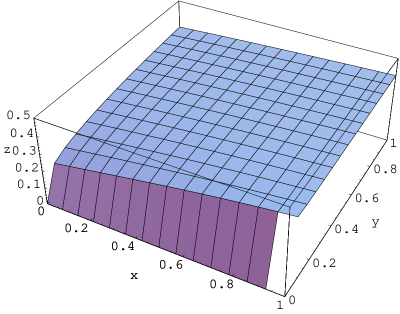
Figure 1: A plot of the relative entropy perturbation $\mathcal{S}_{mr}/(3\,\zeta)$ ($z$-axis) as a function of $\Gamma_{m}^{1}\cdot t_{0}$ ($x$-axis) and $\Gamma_{r}^{0}\cdot t_{0}$ ($y$-axis). For a large set of decay rates, isocurvature perturbations are significant. Note that $\Gamma_{m}^{1}\cdot t_{0}=0$ or $\Gamma_{r}^{0}\cdot t_{0}=0$ are ill-defined limits (there is no decay into matter or radiation).

A feature of this concrete example that I expect to survive in models with less assumptions is the linear dependence of the matter density perturbations on the initial density perturbation $\delta\rho_{0}$. Hence, if entropy perturbations originate from reheating after single field inflation, the spectral indices of entropy and curvature perturbations should be identical, and entropy and curvature modes should be also completely correlated. Though this seems plausible and might simply follow from linearity of the equations, as I mentioned at the beginning one should be cautious to generalize statements only known to apply in particular cases.

Although our example does indeed contain non-adiabatic perturbations, the Bardeen variable $\zeta$ remains constant on large scales, Eq. (12). This happens because all components have the same equation of state. The last feature though was introduced in the counter-example merely to simplify the equations, and it is likely that if the assumption ${w_{\alpha}=w_{\beta}}$ is dropped while maintaining the non-universal time-dependence of the decay rates, isocurvature perturbations are still going to be generated during reheating.

But even if we maintain the assumption of common equation of state during reheating, it is possible to generate changes in $\zeta$ on large scales. Suppose for instance that the inflaton decays into radiation ($r$) and a sufficiently light species of dark matter particles ($m$). Though dark matter might behave as a relativistic component during reheating ($w_{m}\approx 1/3$), once its temperature later drops below its mass, it will start behaving as a pressureless component $w_{m}\approx 0$. The non-vanishing (and constant) entropy perturbation $\mathcal{S}_{mr}$ will then, since ${w_{m}\neq w_{r}}$, source changes in $\zeta$ on large scales and have a significant impact on structure formation Wayne .

III Conclusion

In order to show that single-field inflation does not generically produce a spectrum of adiabatic perturbations, it is sufficient to present a single counter-example. In this paper, I have described a toy reheating process that yields significant amounts of non-adiabatic perturbations after single-field inflation. The example contains several ingredients. Some of them them are superfluous, and their sole purpose is to simplify the analysis. Others are essential, and their presence alone is likely to produce non-adiabatic perturbations during reheating. The essential ingredient here is the “non-universal” spacetime dependence of the rates at which the inflaton decays into different components. Obviously, such an asymmetric dependence can only occur if the inflaton decays into more than one fluid (radiation and dark matter for instance). As a caveat, let me mention that I have neglected spatial divergences of the momentum and the shear gradient in the equations of motion for the perturbations. These terms are expected to be negligible in the long-wavelength limit, though in order to rigorously asses their importance, one should deal with equations of motion containing a single variable Mukhanov .

Is such a non-universal behavior of the decay rates expected to occur in realistic models? The universe contains several constituents, like baryons, dark matter, photons, neutrinos and quintessence, so there is no reason for the inflaton to decay into a single component. In addition, reheating proceeds in different stages. Initially, parametric amplification is responsible for an explosive production of particles known as preheating and subsequently, the inflaton decays by conventional (and essentially different) perturbative processes KoLiSt . During this last stage of reheating particles might also acquire thermal masses, which again render the inflaton decay rate spacetime-dependent KNR . Therefore, it is extremely plausible that the inflaton decay rate could depend on spacetime quantities MatarreseRiotto . On top of that, the decay products of the inflaton might be very different, like dark matter and radiation are, so there is no reason to assume that their couplings to the inflaton and, hence, their corresponding creation rates are related to each other. Overall, it might very well be that the decay rates evolve in a non-universal way. In that case, rather than a spectrum of adiabatic perturbations, the signature that points to the single-field origin of the entropy perturbations in our example is the complete correlation of entropy and curvature modes, and the common spectral index.

The counter-example presented here does not imply that single-field inflation is in conflict with observations. First, significant amounts of isocurvature are still allowed by experiment CGBLR . Second, there are models where perturbations still remain adiabatic after reheating. In fact, the mechanism I have described can be regarded from a different perspective. Little is known about the physics of reheating. Hence, the possibility that isocurvature perturbations can be efficiently produced during reheating might, together with observational constraints, shed a fair amount of light into our understanding and modeling of the reheating process after a stage of single-field inflation.

IV Note added in proof

After this preprint was posted on the archive, S. Weinberg and S. Bashinsky kindly pointed out to me that, under quite general assumptions, the adiabaticity of the perturbations generated during a stage of single-field inflation follows from the results presented in Weinberg1 and BashinskySeljak . As suggested by them, the origin of the non-adiabatic perturbations discussed here is the discontinuous change of the decay rate along a spatial hypersurface where the total energy density is perturbed Weinberg2 . Such a change makes the perturbations non-adiabatic already at the beginning of reheating. The nature of the perturbations generated during a stage of single-field inflation is specifically analyzed in Weinberg2 .

- (1) H. V. Peiris et al., “First year Wilkinson Microwave Anisotropy Probe (WMAP) observations: Implications for inflation,” Astrophys. J. Suppl. 148, 213 (2003) [arXiv:astro-ph/0302225].
- (2) M. Tegmark et al. [SDSS Collaboration], “Cosmological parameters from SDSS and WMAP,” arXiv:astro-ph/0310723.
- (3) A. D. Linde, “Particle Physics and Inflationary Cosmology,” Harwood (Chur, Switzerland), (1990). D. H. Lyth and A. Riotto, “Particle physics models of inflation and the cosmological density perturbation,” Phys. Rept. 314, 1 (1999) [arXiv:hep-ph/9807278].
- (4) L. H. Ford, “Inflation Driven By A Vector Field,” Phys. Rev. D 40, 967 (1989).
- (5) M. Bucher, A. S. Goldhaber and N. Turok, “An open universe from inflation,” Phys. Rev. D 52, 3314 (1995) [arXiv:hep-ph/9411206].
- (6) A. D. Linde and A. Mezhlumian, “Inflation with Omega not = 1,” Phys. Rev. D 52, 6789 (1995) [arXiv:astro-ph/9506017].
- (7) F. Lucchin and S. Matarrese, “Power Law Inflation,” Phys. Rev. D 32, 1316 (1985).
- (8) A. D. Linde and V. Mukhanov, “Nongaussian isocurvature perturbations from inflation,” Phys. Rev. D 56, 535 (1997) [arXiv:astro-ph/9610219].
- (9) A. D. Linde, “Generation Of Isothermal Density Perturbations In The Inflationary Universe,” Phys. Lett. B 158, 375 (1985).
- (10) V. F. Mukhanov and G. V. Chibisov, “Quantum Fluctuation And ’Nonsingular’ Universe. (In Russian),” JETP Lett. 33, 532 (1981) [Pisma Zh. Eksp. Teor. Fiz. 33, 549 (1981)]. S. W. Hawking, “The Development Of Irregularities In A Single Bubble Inflationary Universe,” Phys. Lett. B 115, 295 (1982). A. A. Starobinsky, “Dynamics Of Phase Transition In The New Inflationary Universe Scenario And Generation Of Perturbations,” Phys. Lett. B 117, 175 (1982). A. H. Guth and S. Y. Pi, “Fluctuations In The New Inflationary Universe,” Phys. Rev. Lett. 49, 1110 (1982). J. M. Bardeen, P. J. Steinhardt and M. S. Turner, “Spontaneous Creation Of Almost Scale - Free Density Perturbations In An Inflationary Universe,” Phys. Rev. D 28, 679 (1983).
- (11) D. Wands, K. A. Malik, D. H. Lyth and A. R. Liddle, “A new approach to the evolution of cosmological perturbations on large scales,” Phys. Rev. D 62, 043527 (2000) [arXiv:astro-ph/0003278]. Ibid., “Superhorizon perturbations and preheating,” arXiv:astro-ph/0010639.
- (12) L. Kofman, A. D. Linde and A. A. Starobinsky, “Towards the theory of reheating after inflation,” Phys. Rev. D 56, 3258 (1997) [arXiv:hep-ph/9704452].
- (13) K. A. Malik, D. Wands and C. Ungarelli, “Large-scale curvature and entropy perturbations for multiple interacting fluids,” Phys. Rev. D 67, 063516 (2003) [arXiv:astro-ph/0211602].
- (14) H. Kodama and M. Sasaki, “Cosmological Perturbation Theory,” Prog. Theor. Phys. Suppl. 78, 1 (1984).
- (15) S. Matarrese and A. Riotto, “Large-scale curvature perturbations with spatial and time variations of the inflaton decay rate,” JCAP 0308, 007 (2003) [arXiv:astro-ph/0306416].
- (16) A. Mazumdar and M. Postma, “Evolution of primordial perturbations and a fluctuating decay rate,” Phys. Lett. B 573, 5 (2003) [arXiv:astro-ph/0306509].
- (17) F. Finelli and R. H. Brandenberger, “Parametric amplification of gravitational fluctuations during reheating,” Phys. Rev. Lett. 82, 1362 (1999) [arXiv:hep-ph/9809490]. Id., “Parametric amplification of metric fluctuations during reheating in two field models,” Phys. Rev. D 62, 083502 (2000) [arXiv:hep-ph/0003172].
- (18) S. Gupta, K. A. Malik and D. Wands, “Curvature and isocurvature perturbations in a three-fluid model of curvaton decay,” arXiv:astro-ph/0311562.
- (19) G. Dvali, A. Gruzinov and M. Zaldarriaga, “A new mechanism for generating density perturbations from inflation,” arXiv:astro-ph/0303591.
- (20) L. Kofman, “Probing string theory with modulated cosmological fluctuations,” arXiv:astro-ph/0303614.
- (21) E. W. Kolb, A. Notari and A. Riotto, “On the reheating stage after inflation,” arXiv:hep-ph/0307241.
- (22) M. S. Turner, “Coherent Scalar Field Oscillations In An Expanding Universe,” Phys. Rev. D 28, 1243 (1983).
- (23) D. H. Lyth, “Large Scale Energy Density Perturbations And Inflation,” Phys. Rev. D 31, 1792 (1985).
- (24) P. Crotty, J. Garcia-Bellido, J. Lesgourgues and A. Riazuelo, “Bounds on isocurvature perturbations from CMB and LSS data,” Phys. Rev. Lett. 91, 171301 (2003) [arXiv:astro-ph/0306286].
- (25) W. Hu, “An Isocurvature mechanism for structure formation,” Phys. Rev. D 59, 021301 (1999) [arXiv:astro-ph/9809142].
- (26) V. F. Mukhanov, private communication.
- (27) S. Weinberg, “Adiabatic modes in cosmology,” Phys. Rev. D 67, 123504 (2003) [arXiv:astro-ph/0302326].
- (28) S. Bashinsky and U. Seljak, “Neutrino Perturbations in CMB Anisotropy and Matter Clustering,” arXiv:astro-ph/0310198.
- (29) S. Weinberg, “Can non-adiabatic perturbations arise after single-field inflation?,” arXiv:astro-ph/0401313.