Tracing the Magnetic Field in Orion A

Abstract

We use extensive 350 $\mu$m polarimetry and continuum maps obtained with Hertz and SHARC II along with HCN and HCO⁺ spectroscopic data to trace the orientation of the magnetic field in the Orion A star-forming region. Using the polarimetry data, we find that the direction of the projection of the magnetic field in the plane of the sky relative to the orientation of the integral-shaped filament varies considerably as one moves from north to south. While in IRAS 05327-0457 and OMC-3 MMS 1-6 the projection of the field is primarily perpendicular to the filament it becomes better aligned with it at OMC-3 MMS 8-9 and well aligned with it at OMC-2 FIR 6. The OMC-2 FIR 4 cloud, located between the last two, is a peculiar object where we find almost no polarization. There is a relatively sharp boundary within its core where two adjacent regions exhibiting differing polarization angles merge. The projected angle of the field is more complicated in OMC-1 where it exhibits smooth variations in its orientation across the face of this massive complex. We also note that while the relative orientation of the projected angle of the magnetic field to the filament varies significantly in the OMC-3 and OMC-2 regions, its orientation relative to a fixed position on the sky shows much more stability. This suggests that, perhaps, the orientation of the field is relatively unaffected by the mass condensations present in these parts of the molecular cloud. By combining the polarimetry and spectroscopic data we were able to measure a set of average values for the inclination angle of the magnetic field relative to the line of sight. We find that the field is oriented quite close to the plane of the sky in most places. More precisely, the inclination of the magnetic field is $\approx 73^{\circ}$ around OMC-3 MMS 6, $\approx 74^{\circ}$ at OMC-3 MMS 8-9, $\approx 80^{\circ}$ at OMC-2 FIR 4, $\approx 65^{\circ}$ in the northeastern part of OMC-1, and $\approx 49^{\circ}$ in the Bar. The small difference in the inclination of the field between OMC-3 and OMC-2 seems to strengthen the idea that the orientation of the magnetic field is relatively unaffected by the agglomeration of matter located in these regions. We also present polarimetry data for the OMC-4 region located some $13\arcmin$ south of OMC-1.

1 Introduction

The determination of the orientation of the magnetic field in molecular clouds and their surroundings is important for the assessment of its role and relative importance in the evolution of the clouds and in the process of star formation. Numerous scenarios have been proposed concerning the different stages involved in the birth of stars from primordial clouds (Shu et al., 1987; McKee et al., 1993; Heiles et al., 1993; Mouschovias & Ciolek, 1999; Williams et al., 2000). But, whatever the details, they all seek to describe at some level or another the interaction of the magnetic field with its environment and its influence during gravitational collapse. The magnetic field will resist and slow down the collapse and perhaps even shape the structures observed within the clouds themselves (Fiege & Pudritz, 2000; Matthews, Wilson & Fiege, 2001). Conversely, measurements of the orientation of the magnetic field in molecular clouds and prestellar cores can tell us something about the ways in which cores form; e.g., an hourglass geometry is usually interpreted as a sign of the magnetic field having been dragged by the gas during its collapse (see for example Schleuning (1998)). In that respect, data obtained from polarimetry measurements at far-infrared and submillimeter wavelengths which trace the orientation of the projection of the magnetic field in the plane of the sky (Hildebrand, 1988) are essential for this task and for creating, testing and refining models (Matthews, Wilson & Fiege, 2001).

Recently, Houde et al. (2002) have proposed a new technique that would allow for a more complete determination of the orientation of the magnetic field in that it renders possible the measurement of the inclination or viewing angle that the field makes relative to the line of sight. This is accomplished by combining polarimetry data and ion-to-neutral line width ratios obtained from the spectra of coexistent molecular species. The technique was first applied to the M17 molecular cloud using an extensive 350 $\mu$m Hertz polarimetry map and HCO⁺/HCN spectroscopic data (Houde et al., 2000a, b, 2002), all obtained at the Caltech Submillimeter Observatory (CSO).

We pursue a similar task in this paper where our goal is primarily to use polarimetry and spectroscopic data (as well as continuum maps) to trace the orientation of the magnetic field along the integral-shaped filament (ISF; see Bally et al. (1987)) of the Orion A molecular cloud (OMC). We will use the 350 $\mu$m polarimetry maps obtained with the Hertz polarimeter (Dowell et al., 1998), superposed on SHARC II continuum maps at the same wavelength (Dowell et al., 2003), to study the orientation of the projection of the magnetic field in the plane of the sky along with HCO⁺ and HCN spectra to evaluate the inclination of the field relative to the line of sight.

2 Observations

The core of the data presented in this paper comes from extensive 350 $\mu$m polarimetry maps obtained with the Hertz polarimeter (Dowell et al., 1998) during numerous nights of observations at the Caltech Submillimeter Observatory. In all, seven different regions of the Orion A molecular cloud were studied. They are from north to south: i) IRAS 05327-0457, observed on 2002 February 17-18, ii) OMC-3 MMS 1-6, observed on 1997 September 19, 1998 February 15, 1999 January 27 and 2002 February 18, iii) OMC-3 MMS 8-9, observed on 2002 February 18, iv) the neighborhood of OMC-2 FIR 3-4, observed on 1997 September 19, 1998 February 15 and 1999 January 27, v) the neighborhood of OMC-2 FIR 6, observed on 2002 February 18, vi) OMC-1, observed on numerous nights from 1998 February to 2002 February, and finally vii) OMC-4, observed on 2001 April 16 and 2002 February 18. Although Hertz data provide both polarimetry and continuum maps, we use a SHARC II map for illustrations of the 350 $\mu$m continuum (Dowell et al., 2003). SHARC II has a better spatial resolution than Hertz ($\approx 12\arcsec$ compared to $\approx 20\arcsec$) and the data obtained with it and presented here continuously cover all of the regions mentioned above, unlike the Hertz maps. The SHARC II data were obtained on three separate nights: 2002 November 24, 2003 March 1 and 2003 April 16.

The Hertz data were acquired with conventional azimuth chopping and nodding. The chopper throw ranged from $5\arcmin$ to $8.4\arcmin$, and we made attempts to avoid chopping into known emission sources by choosing the hour angle of the observations. The SHARC II data were acquired with crossing linear scans without chopping the secondary mirror. The data analysis technique subtracts from the source emission a model for the atmospheric emission which is improved through iterations. The total integration time was 3.7 hours in conditions with moderately low zenith opacity ($\tau_{350\mu{\rm{m}}}\sim 1.5$).

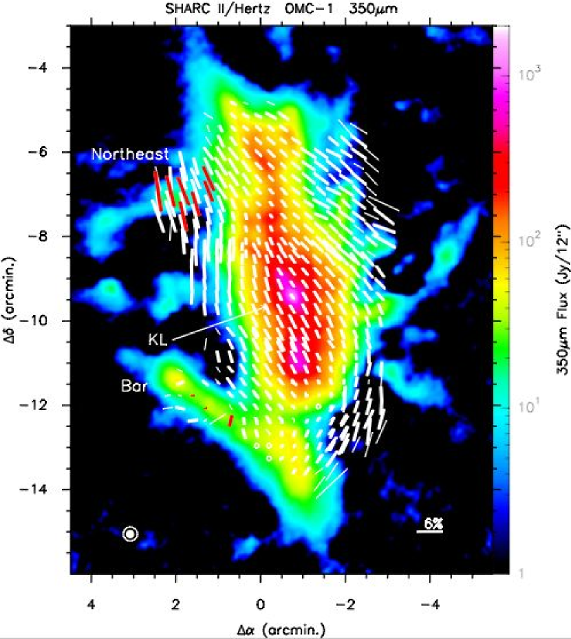
Figure 3: 350 $\mu$m continuum map and polarimetry (E-vectors) of the OMC-1 region obtained with SHARC II and Hertz, respectively. The thick (thin) vectors have a polarization level and uncertainty such that $P\geq 3\sigma_{P}$ ($P\geq 2\sigma_{P}$). Circles indicate cases where $P+2\sigma_{P}<1\%$ and $P<2\sigma_{P}$. The darker polarization vectors denote positions where spectroscopic data were also obtained. The beam widths are shown in the lower left corner, with the solid and open circles for SHARC II at $\simeq 12\arcsec$ and Hertz at $\simeq 20\arcsec$, respectively. The reference position is at R.A.$=5^{h}32^{m}50^{s}$, decl.$=-5\arcdeg 15\arcmin 00\arcsec$ (B1950).

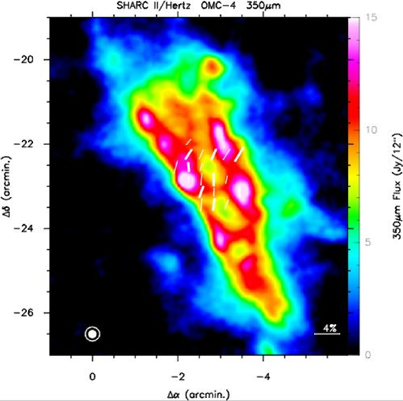
Figure 4: 350 $\mu$m continuum map and polarimetry (E-vectors) of the OMC-4 region obtained with SHARC II and Hertz, respectively. The thick (thin) vectors have a polarization level and uncertainty such that $P\geq 3\sigma_{P}$ ($P\geq 2\sigma_{P}$). The beam widths are shown in the lower left corner, with the solid and open circles for SHARC II at $\simeq 12\arcsec$ and Hertz at $\simeq 20\arcsec$, respectively. The reference position is at R.A.$=5^{h}32^{m}50^{s}$, decl.$=-5\arcdeg 15\arcmin 00\arcsec$ (B1950).

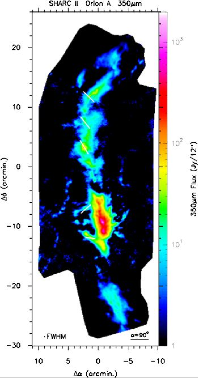
Figure 10: 350 $\mu$m continuum map of the Orion A region obtained with SHARC II. The orientation of the magnetic field is indicated at five positions along the ISF on the map. The projection of the magnetic field in the plane of the sky is also shown by the orientation of the accompanying vectors and the inclination angle is given by the length of the vectors (using the scale shown in the bottom right corner). The beam width is shown in the lower left corner ($\simeq 12\arcsec$) and the reference position is at R.A.$=5^{h}32^{m}50^{s}$, decl.$=-5\arcdeg 15\arcmin 00\arcsec$ (B1950).

We present in Figure 1 the northern portion of the data where the polarimetry measurements for IRAS 05327-0457 and OMC-3 are plotted on top of the SHARC II continuum map. Figures 2, 3 and 4 present the same type of data but for the OMC-2, OMC-1 and OMC-4 regions, respectively. For each of these figures, the thick (thin) polarization vectors have a polarization level and uncertainty such that $P\geq 3\sigma_{P}$ ($P\geq 2\sigma_{P}$), circles indicate cases where $P+2\sigma_{P}<1\%$ and $P<2\sigma$, and the darker polarization vectors and circles denote positions where spectroscopic data were also obtained. The beam widths are shown in the lower left corner, with the solid and open circles for SHARC II and Hertz, respectively. The complete unbroken SHARC II continuum map can be seen in Figure 10. Because of the very low levels of polarization observed on some of the sources studied in this paper, we have decided to include data points that have an uncertainty in their polarization level better or equal to $2\sigma$ instead of the usual $3\sigma$ common to Hertz papers (see for example Houde et al. (2002)). The set of polarization angles measured for these $2\sigma$ points have an uncertainty $\lesssim 15^{\circ}$, as opposed to $\lesssim 10^{\circ}$ for $3\sigma$ points, and agree well with adjacent points of lower uncertainty. Their inclusion will not affect the conclusions drawn later. Details of the polarimetry data will be found in Tables 2 to 5.

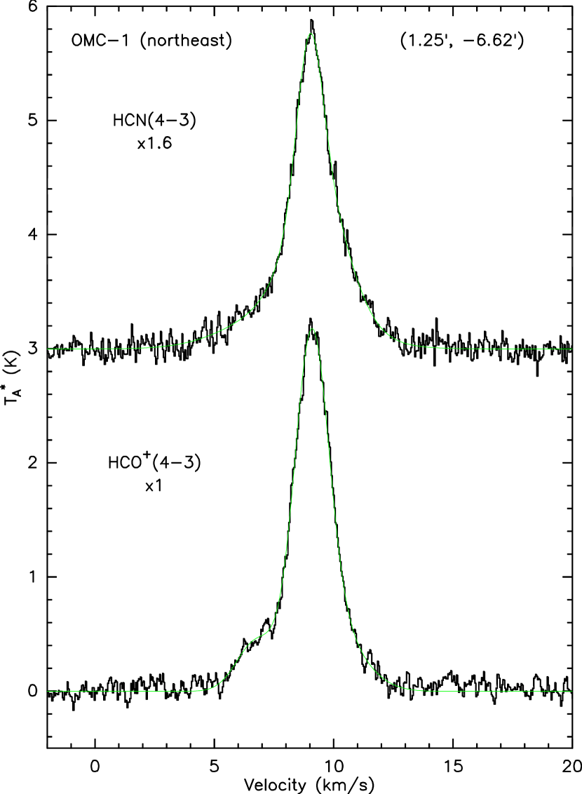
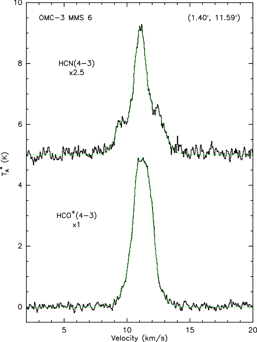
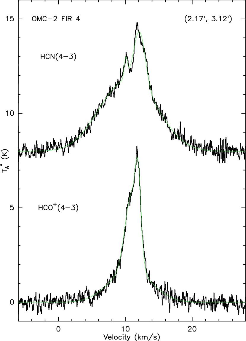
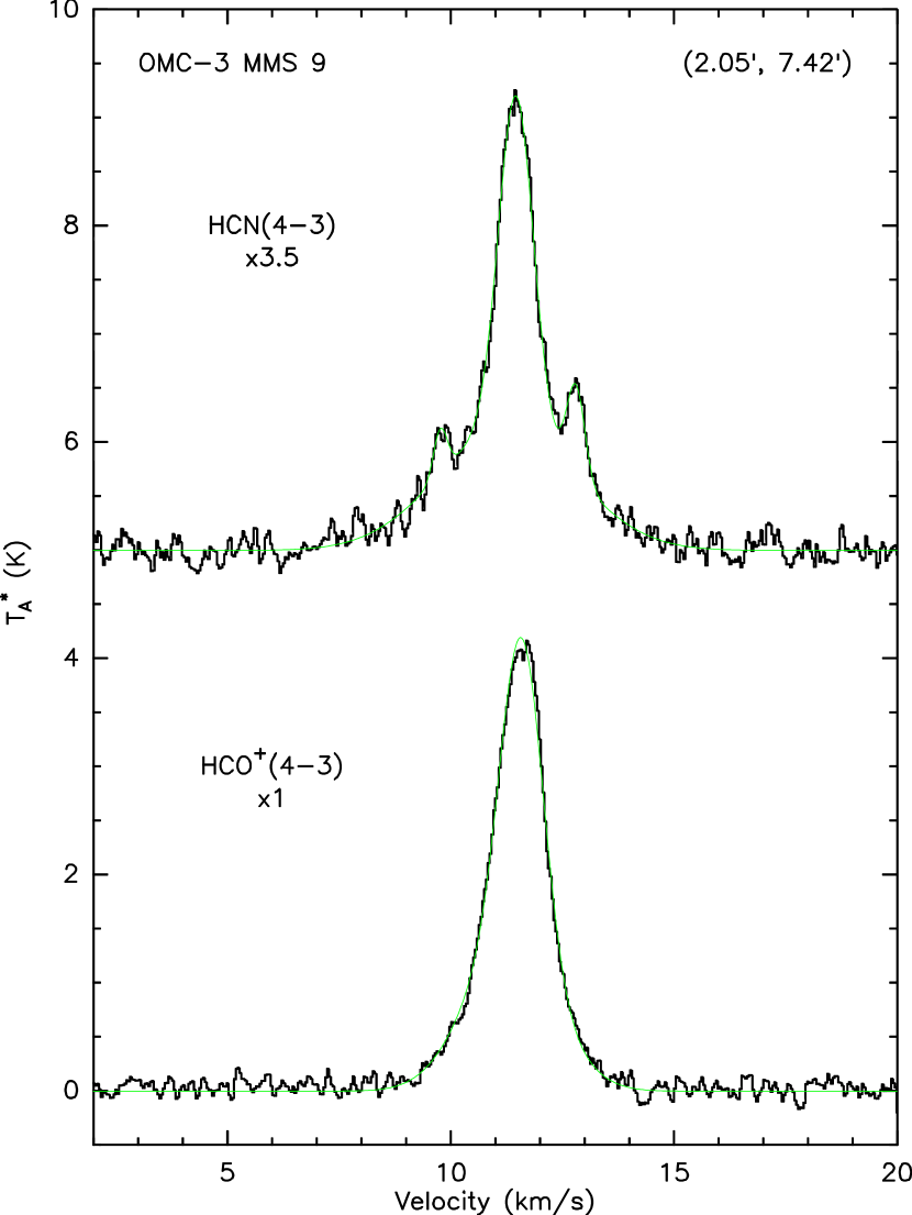
Figure 5: HCN and HCO⁺ spectra in the $J=4\rightarrow 3$ transition for, from top-left and clockwise, OMC-1 (northeast), OMC-3 MMS 6, OMC-3 MMS 9 and OMC-2 FIR 4, respectively. The offset position from the reference at R.A.$=5^{h}32^{m}50^{s}$, decl.$=-5\arcdeg 15\arcmin 00\arcsec$ (B1950) (see Figure 10) is given in the upper right corner of each pair of spectra, in arcminutes.

We have also measured HCN and HCO⁺ spectra in the $J=4\rightarrow 3$ transition at different positions along the ISF; these are necessary to evaluate the inclination angle of the magnetic field relative to the line of sight. In all, twenty-seven such pairs of spectra were obtained using the 300-400 GHz Receiver of the CSO: three in the Bar, seven in the northeastern part of OMC-1, seven in OMC-2 FIR 4, five in and around OMC-3 MMS 6 and five in OMC-3 MMS 8-9. In the latter, two of the five points do not have corresponding polarimetry vectors with $P\geq 2\sigma_{P}$ or $P+2\sigma_{P}<1\%$ and are identified with dark dots in Figure 1. Typical examples of measured HCN and HCO⁺ spectra, along with a fit to their profiles, can be found in Figure 5. This set of data was obtained during numerous nights of observation at the CSO on 2002 September, 2002 December, 2003 January to 2003 April and 2003 August.

3 Results

3.1 The 350 $\mu$m SHARC II map

Although our analysis will concentrate on the nature of the magnetic field in Orion A, it is appropriate at this point to say a few words concerning the 350 $\mu$m SHARC II continuum map presented in Figure 10. The Orion A molecular cloud has been mapped at several wavelengths in the past and we do not intend to repeat the work presented in other papers. For example, Lis et al. (1998) also published a 350 $\mu$m map of this region, obtained with SHARC, and gave a detailed analysis of the physical conditions found in the different parts of the cloud as well as a list (in their Table 1) of the sources that can be found in OMC-2 and OMC-3 (see also Chini et al. (1997) for observations at 1.3 mm of the OMC-2 and OMC-3 regions). Our map covers the same area as that of Lis et al. (1998) but also extends further both north of OMC-3 and south of OMC-1, and is wider in its east-west coverage. More precisely, our map includes the neighborhood of IRAS 05327-0457 (Makinen et al., 1985; Mookerjea et al., 2000a, b) which extends some $\approx 4\arcmin$ north of OMC-3 MMS 1. It is in fact seen to be an extension of the OMC-3 MMS 1-6 filament that branches off to the north in a region of higher flux located at $\Delta\alpha\simeq\mathrm{-3}\arcmin$ and $\Delta\delta\simeq\mathrm{1}7\arcmin$ on Figure 10. This extension then turns southeast in a direction parallel to the OMC-3 MMS 1-6 complex and ends up at the CSO 1 condensation of Lis et al. (1998) at $\Delta\alpha\simeq\mathrm{3}\arcmin$ and $\Delta\delta\simeq\mathrm{14.4}\arcmin$ (better seen on Figure 1). This IRAS 05327-0457 region was also part of an extensive 850 $\mu$m SCUBA map published by Johnstone & Bally (1999) and our results are seen to be in qualitative agreement with theirs. The same can be said of the V-shaped OMC-4 region (Johnstone & Bally, 1999), located some $\approx 13\arcmin$ south of the KL Nebula of OMC-1, and of the whole extent of the two maps, i.e., theirs and ours, which have a similar coverage.

The sensitivity varies somewhat across the SHARC II image due to variable integration time and weather conditions. For most of the regions including OMC-1, OMC-2 and OMC-3, the RMS is approximately $1\,{\rm{Jy}}/12\arcsec$ beam, with higher noise at the edges of the rectangular region of coverage. For the IRAS05327-0457 and OMC-4 fields, the RMS is approximately $0.3\,{\rm{Jy}}/12\arcsec$ beam.

3.2 The polarimetry data

3.2.1 The IRAS 05327-0457 and OMC-3 regions

Figure 1 shows a close-up of the IRAS 05325-0457 and OMC-3 fields from the SHARC II map along with the Hertz polarization vectors obtained in three different regions: IRAS 05327-0457, OMC-3 MMS 1-6 and OMC-3 MMS 8-9. One thing to notice about the first two regions is that the general orientation of the polarization vectors is in both cases well aligned with, or similarly that the magnetic field is practically perpendicular to the local filaments. Indeed, if we visually estimate the orientation of the filaments, we find that both IRAS 05327-0457 and OMC-3 MMS 1-6 are aligned at approximately $132^{\circ}$ (east from north, as will always be the case for all angles measured in the plane of the sky). On the other hand, a simple arithmetic mean of the polarization angle ($PA$) of the vectors in both regions gives $\simeq 142^{\circ}\pm 18^{\circ}$ for IRAS 05327-0457 and $\simeq 137^{\circ}\pm 9^{\circ}$ for OMC-3 MMS 1-6, respectively. These values are practically unchanged if we instead average the Stokes parameters from the same ensembles of points, we then get $\left\langle PA\right\rangle\simeq 143^{\circ}\pm 3^{\circ}$ for IRAS 05327-0457 and $\left\langle PA\right\rangle\simeq 136^{\circ}\pm 1^{\circ}$ for OMC-3 MMS 1-6, respectively. Since these two types of averages usually agree well, and that we will later deal with objects exhibiting low polarization levels, we will for now on only use Stokes averages. The difference between the orientation of the polarization vectors and the local filaments is on average only approximately $5^{\circ}$ to $10^{\circ}$ for these two regions, i.e., they are well aligned with each other. A similar result has already been reported for the OMC-3 MMS 1-6 region by Matthews, Wilson & Fiege (2001) using SCUBA at 850 $\mu$m (see their Figure 2). The fact that the same is true for IRAS 05327-0457 adds credence to their suggestion that perhaps the ordered structure of the magnetic field has not been disturbed or deflected by the gravitational collapses of the protostellar cores present in these regions (Chini et al., 1997).

OMC-3 MMS 8-9 is the third region in Figure 1 where we have obtained polarimetry data. As was noticed by Matthews, Wilson & Fiege (2001) at 850 $\mu$m, we find that, as compared to the case of OMC-3 MMS 1-6, the orientation of the polarization vectors has significantly changed in relation to the local filament. This part of the ISF is oriented at $\approx 8^{\circ}$, roughly a $60^{\circ}$ shift relative to OMC-3 MMS 1-6. The polarization angle calculated with the average of the Stokes parameters yields $\left\langle PA\right\rangle\simeq 122^{\circ}\pm 2^{\circ}$. But since OMC-3 MMS 8-9 exhibits a significant amount of flux both east and west of the main core, a case could be made in favor of limiting ourselves only to vectors located strictly in the core (i.e., the polarization vectors situated on the ten positions of highest local flux around $\Delta\alpha\simeq 2\arcmin$ and $\Delta\delta\simeq 7.5\arcmin$) before calculating the Stokes averages. It turns out, however, that the change is not significant when we do so as we then obtain $\left\langle PA\right\rangle\simeq 129^{\circ}\pm 3^{\circ}$. Therefore, depending on which number we use we find that the vectors are misaligned by approximately $114^{\circ}$ to $121^{\circ}$ in relation to the filament. This is somewhat more than the mean of $86^{\circ}$ measured by Matthews, Wilson & Fiege (2001) at 850 $\mu$m; the difference may lie in the fact that our vectors located east of the main core do not change appreciably from those located in the core, as seems to be the case for the SCUBA data. At any rate, this represents a significant change when compared to what was obtained in IRAS 05327-0457 and OMC-3 MMS 1-6.

But perhaps the most important thing to stress from these results is that the average polarization angle does not change much from IRAS 05327-0457 to OMC-3 MMS 1 to OMC-3 MMS 8- 9. Indeed the change is only $\approx 13^{\circ}$. Since it is believed that, at the wavelengths dealt with here, the orientation of the magnetic field projected in the plane of the sky is perpendicular to that of the polarization vectors (Hildebrand, 1988), the same can be said of the projected direction of the field. One must somewhat temper this assertion as there is some indication from the 850 $\mu$m data of Matthews, Wilson & Fiege (2001) that the orientation of the polarization vectors measured between OMC-3 MMS 6 and OMC-3 MMS 7 follows the changing orientation of the filament. This could increase the dispersion in the orientation of the polarization vectors when measured over the field presented in Figure 1.

Finally, we end this section with a few words concerning the polarization levels detected in these parts of the ISF. We find that the percentage of polarization is typical of what is usually observed with Hertz at 350 $\mu$m as $0\%\lesssim P\lesssim 5\%$, with the highest levels detected in IRAS 05327-0457 and the lowest levels in OMC-3 MMS 8-9. This is also reflected in the Stokes averaged polarization levels, which are $2.33\%\pm 0.37\%$, $1.55\%\pm 0.12\%$ and $1.02\%\pm 0.10\%$ for IRAS 05327-0457, OMC-3 MMS 1-6 and OMC-3 MMS 8-9, respectively.

3.2.2 The OMC-2 region

We present with Figure 2 the section of the SHARC II map that is centered on the OMC-2 region along with the polarization data obtained with Hertz in and around OMC-2 FIR 3-4 and FIR 6. This region is characterized, amongst other things, by a gradual change in the orientation of the filament. While in the northern part of the map the filament makes an angle of $\approx 160^{\circ}$ relative to north, it goes through the north-south orientation at OMC-2 FIR 4 and ends at $\approx 35^{\circ}$ (or $\approx 215^{\circ}$) at OMC-2 FIR 6. A visual inspection of the map allows us to quickly evaluate the general characteristics of the polarimetry data. First, just north of OMC-2 FIR 4 the polarization vectors seem to be well aligned with the filament but not with the vectors measured in the OMC-3 field. Second, OMC-2 FIR 4 displays very little polarization which at first renders it impossible to safely determine any relative alignment in this region. This is probably the object which exhibits the lowest levels of polarization amongst all of those observed with Hertz so far. Although a strong depolarization effect, defined by a systematic decrease in polarization level with increasing continuum flux, is commonly seen in this type of study (Dotson, 1996; Matthews, Wilson & Fiege, 2001; Houde et al., 2002), this is probably the most severe case to date. Finally, the orientation of the vectors changes one more time around OMC-2 FIR 6 where they appear to be perpendicular to the filament.

We can quantify these observations by, once again, calculating the averaged Stokes parameters (it would be unwise to attempt anything else with the OMC-2 FIR 4 data) and deriving values for the polarization angle in these parts of the ISF. We find that $\left\langle PA\right\rangle\simeq 175^{\circ}\pm 3^{\circ}$ for the region adjacent to and north of OMC-2 FIR 3 (for $\Delta\delta\mathrm{>3.4}\arcmin$), $\left\langle PA\right\rangle\simeq 121^{\circ}\pm 5^{\circ}$ for the core of OMC-2 FIR 4 (for $2.8\arcmin<\Delta\delta\mathrm{<3.4}\arcmin$) and $\left\langle PA\right\rangle\simeq 115^{\circ}\pm 6^{\circ}$ for OMC-2 FIR 6. These give the following differences between the mean orientation of the vectors and the filament: $\approx 15^{\circ}$, $\approx 59^{\circ}$ and $\approx 80^{\circ}$, in the same order.

It is interesting to note that there appears to be a relatively sharp transition close to the position of peak intensity of OMC-2 FIR 4 ($\Delta\delta\simeq\mathrm{3.}1\arcmin$) where the polarization angle changes abruptly from its FIR 6 value ($\approx 115^{\circ}$, i.e., almost perpendicular to the local orientation of the filament) to the FIR 3 value ($\approx 175^{\circ}$, i.e., almost parallel to the local orientation of the filament). One might hope to explain the unusually low level of polarization measured at OMC-2 FIR 4 by combining the measurements obtained on either side of this boundary. We could expect, for example, a drop in the polarization level at OMC-2 FIR 4 if the polarization patterns north and south of it preserve their relative orientation to the filament as they merge toward it (for comparable polarized flux). The Stokes averaged polarization levels calculated for OMC-2 FIR 6 and OMC-2 FIR 3 are $0.91\%\pm 0.28\%$ and $0.73\%\pm 0.14\%$, respectively; we were unable to reproduce the result obtained for FIR 4 ($0.35\%\pm 0.08\%$) by combining them (along with their corresponding mean polarization angle and flux).

As was the case for the OMC-3 region, we find that the orientation of the average polarization angle does not vary much between OMC-2 FIR 4 and OMC-2 FIR 6 ($\approx 6^{\circ}$) and is also not very different to the values measured in OMC-3. In fact, neglecting the field adjacent to and north of OMC-2 FIR 3, we find a smooth decrease from the north of OMC-3 (or IRAS 05327-0457) to the south of OMC-2.

We note finally that the boundary where the jump in the orientation of the polarization angle occurs is almost coincident with a region in the vicinity of OMC-2 FIR 3 where intense outflow activity is detected. According to Williams et al. (2003), this source is composed of a binary which drives a pair of criss-crossed flows oriented at $\approx 30^{\circ}$, similar to the orientation of the projection of the magnetic field in the plane of the sky at and south of OMC-2 FIR 4. Moreover, there is also some evidence for another flow, in the same neighborhood, oriented at $\approx 80^{\circ}$ in the plane of the sky (J. P. Williams, private communication), this is again very close to the orientation of the field at and north of OMC-2 FIR 3.

3.2.3 The OMC-1 and the Bar regions

We present in Figure 3 a section of the SHARC II map centered on the OMC-1 region along with the polarization data obtained with Hertz superposed on the continuum. A quick glance will suffice to convince the reader of the totally different orientation of the polarization vectors measured in this field when compared to those of the OMC-3 and OMC-2 regions. A small subset of the polarimetry data, centered in the neighborhood of the KL Nebula (at $\Delta\alpha\simeq\mathrm{-0.7}\arcmin$ and $\Delta\delta\simeq\mathrm{-9.4}\arcmin$ on Figure 3), has already been published by Schleuning (1998) along with an extensive 100 $\mu$m map, albeit at a lower resolution, of the OMC-1 cloud. The polarization pattern was then interpreted as being consistent with that produced by a magnetic field shaped like an hourglass (see Figure 4 of Schleuning (1998)) resulting from the gravitational distortion caused by the IRc 2 Ridge. Eight positions in OMC-1 have also been measured in polarimetry by Vall e & Bastien (1999) at 760 $\mu$m. The polarization angles are quite comparable, within uncertainties, except for two positions which do not agree. Usually, the polarization levels are also similar, or somewhat larger at 760 $\mu$m (within a beam width of $\approx 14\arcsec$).

Although our 350 $\mu$m polarimetry map qualitatively agrees well with the 100 $\mu$m counterpart, there are a few differences and features in the new set of data that complicate the interpretation. This is especially true in the southern part of the map, most notably in and around the Bar where there is a significant change in the orientation of the vectors (more on this below) that does not fit with the hourglass interpretation. There is also a difference in the region east of the Ridge where the magnetic field on our map appears to be basically aligned along an east-west axis. But, all in all, there is an unmistakable pinch in the orientation of the magnetic field in the neighborhood of the Ridge with the region of largest curvature located just north of the KL Nebula. But as was stated by Rao et al. (1998), caution must be used in interpreting the orientation of the magnetic field from polarimetry data in regions of high outflow activity, as is the case for the Ridge. This is owed to the possibility that, in the presence of outflows, grains can be aligned with their long axis parallel to the magnetic field through the Gold alignment mechanism (Gold, 1952; Lazarian, 1994, 1997). Incidentally, our data also show the existence of the “polarization hole” in the vicinity of the KL Nebula that was shown by Rao et al. (1998) to be caused by an abrupt and small scale $90^{\circ}$ change in the orientation of the polarization vectors and presumably caused by the presence of outflows, as was just mentioned. This, however, is not the only place where a local decrease of the polarization level is seen. The same is true, for example, in the neighborhood of i) the Bar, ii) in a relatively large region in the south of the map, and west of the Bar, centered at $\Delta\alpha\simeq\mathrm{-1.0}\arcmin$ and $\Delta\delta\simeq\mathrm{-12.4}\arcmin$ or again iii) some $2\arcmin$ north of KL at $\Delta\alpha\simeq\mathrm{-0.2}\arcmin$ and $\Delta\delta\simeq\mathrm{-7.5}\arcmin$ (a local peak in the continuum flux).

As was said earlier, the overall orientation of the polarization vectors in OMC-1 is totally different from what we have seen so far in Orion A. By doing averages of Stokes parameters on small ensembles of points we find that the polarization angle changes significantly as one moves about the cloud. Although in the north of the map the vectors converge to an orientation of $\approx 40^{\circ}$ (somewhat different from the $\approx 30^{\circ}$ measured around the KL Nebula, in agreement with previous results (see Table 1 of Schleuning (1998)), the polarization angle is seen to cover values anywhere from $\approx 0^{\circ}$ east of the Ridge to $\approx 60^{\circ}$ in the northwestern corner of the map to $\approx 160^{\circ}$ in the southwestern corner. The southern part of the map, and the Bar in particular, is where we find the most abrupt changes in the orientation of the vectors. A Stokes average of eighteen data points located in the Bar gives a mean polarization angle of $\left\langle PA\right\rangle\simeq 82^{\circ}\pm 4^{\circ}$.

The polarization levels also greatly vary across OMC-1. The lowest levels are found in the south of the map where a few positions with no polarization (i.e., where $P+2\sigma_{P}<1\%$ and $P<2\sigma_{P}$) are found. The mean polarization level found in the Bar, using the same eighteen points as before, is $\left\langle P\right\rangle=0.76\%\pm 0.14\%$. Schleuning (1998) interpreted this low level as being caused by a local orientation of the magnetic field along the line of sight as a result of being pushed out of the M42 H II region. But as will be discussed in section 3.3.1, our measurements for the inclination of the magnetic field in this region are not in agreement with this interpretation. An alternative explanation could reside in the fact that the dust is colder in the Bar than in other regions of higher flux in OMC-1, thus its lower levels of polarization would be consistent with the hypothesis that cooler dust is intrinsically less polarized (Vaillancourt, 2002). On the other hand, we also find in OMC-1 some of the largest polarization levels ever detected with Hertz at 350 $\mu$m. For example, the group of dark colored vectors in the northeastern part of Figure 3 have levels that can reach as high as $\approx 10$%. These levels are found in a region of relatively low flux where the depolarization effect is minimal and will be useful for our measurement of the angle of inclination of the magnetic field that will soon follow.

3.2.4 The OMC-4 region

Finally, as far as the polarimetry data are concerned, we show in Figure 4 the Hertz polarization vectors superposed on the SHARC II continuum map of OMC-4. It is located some $13\arcmin$ south of the KL Nebula in OMC-1 and is seen to be of relatively low intensity ($\approx 10$ Jy in $12\arcsec$). An average of the Stokes parameters for a few vectors gives a polarization level of $\approx 1.5$% and a polarization angle of $\approx 165^{\circ}$. Although the amount of polarization measured is similar to what was found in IRAS 05327-457 and OMC-3 MMS 1-6, the orientation of the vectors exceeds what is found there by some $20^{\circ}$ to $30^{\circ}$. Moreover, their orientation does not follow the general orientation of the local filament which makes an angle of approximately $25^{\circ}$.

3.3 The spectroscopic data - the inclination angle of the magnetic field

In this section we will make use of the technique put forth by Houde et al. (2002) that allows for a measurement of the inclination of the magnetic field relative to the line of sight. We present in Figure 5 typical spectra (although see section 3.3.3) taken in four of the five regions where we have sought and obtained spectroscopic data: the northeastern part of OMC-1, and the neighborhoods of OMC-3 MMS 6, OMC-3 MMS 9 and OMC-2 FIR 4. The technique relies on comparisons of line profiles of coexistent neutral and ion molecular species and we have chosen the $J\rightarrow 4-3$ transition of HCN and HCO⁺, respectively. The telescope beam width was $\approx 20\arcsec$ for these observations, similar to that obtained while observing with Hertz.

3.3.1 Calibration of the ion-to-neutral line width ratio and the calculation of the inclination angle

As was explained by Houde et al. (2002), the evaluation of the inclination angle of the magnetic field necessitates the combination of spectroscopic and polarimetry data. This is done by effectively calibrating the ion-to-neutral line width ratio, calculated a priori from the HCO⁺ and HCN spectra, with the corresponding polarimetry data. In doing so, one tries to determine the most suitable of a family of curves, pertaining to the propensity of alignment between the magnetic field and neutral flows, to apply to the region under study (see the models of Figures 2, 4 and 5 of Houde et al. (2002)). For the present case of Orion A, ideally one would like to determine such a curve for each region where one desires to locally evaluate the inclination angle (which will be labeled $\alpha$, along with $\beta$ for the angle made by the projection of the magnetic field on the plane of the sky). Unfortunately, the strong amount of depolarization encountered in most of the regions studied here renders this task impossible. This can be asserted from Figure 6 where we plotted the polarization level against the 350 $\mu$m continuum flux for the polarimetry data shown for the OMC-3 and OMC-2 fields of Figures 1 and 2, respectively. Since our spectroscopic data had to be taken in locations of high enough intensity, the corresponding polarimetry points are all significantly affected by the depolarization effect.

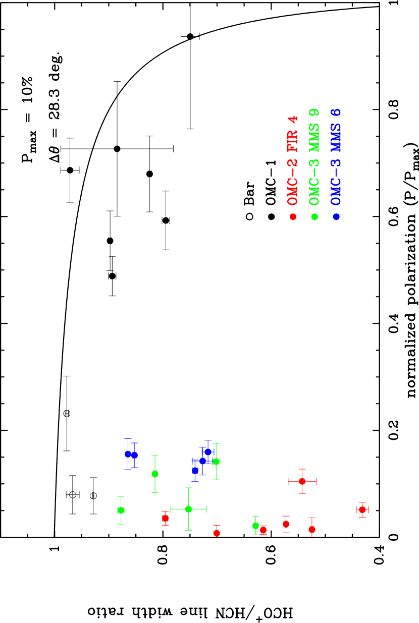
Figure 7: The HCO⁺/HCN line width ratio vs the normalized polarization level ($P/P_{max}$) for Orion A. $P_{max}$ is set at 10% and the data are shown against a model of neutral flow collimation of $\Delta\theta=28.3^{\circ}$(solid curve). The high level of depolarization in OMC-3 and OMC-2 is clearly seen. The polarization vectors used to determine the model all have $P>3\sigma_{P}$.

Faced with this, one could reasonably choose an arbitrary curve corresponding to the aforementioned set of models (defined by the $\Delta\theta$ parameter of equation (11) of Houde et al. (2002), which quantifies the level of collimation of the neutral flows to the magnetic field). Although this would bring some uncertainty in the evaluation of $\alpha$, it should give a reasonably good estimate. This is especially true if $\alpha$ covers a set of values that are close to the lower and upper limits of its available range (i.e., $0^{\circ}$ and $90^{\circ}$, respectively; see the discussion in section 5 of Houde et al. (2002)). There was, however, another option available to us. Although the OMC-1 field is also severely depolarized at places, there exists regions away from the core where the flux is high enough and the depolarization weak enough to allow us to use the polarization levels measured there to calibrate the data for all of Orion A. In fact, as stated before, OMC-1 presents us with some of the highest polarization levels ever measured with Hertz. We, therefore, chose for this seven such points for which the corresponding polarization vectors were plotted in a darker color in Figure 3 (around $\Delta\alpha\simeq\mathrm{1.5}\arcmin$ and $\Delta\delta\simeq\mathrm{-7}\arcmin$). The result of the calibration is shown in Figure 7 where we have set the maximum level of polarization $P_{max}$ to $10\%$. Houde et al. (2002) had chosen $P_{max}=7\%$ in their study of the magnetic field in M17, but we obviously had to update this parameter in view of our more recent data. This parameter, just as $\Delta\theta$, has been shown not to have a significant impact on the results. The model that best fits our data, using a non-linear least-squares technique, has $\Delta\theta=28.3^{\circ}$ as shown in Figure 7.

This analysis allows us to give a set of average values for $\alpha$ in the five regions studied here. More precisely, we obtain from simple averages $\alpha\simeq 72.6^{\circ}\pm 4.4^{\circ}$, $\simeq 73.7^{\circ}\pm 5.2^{\circ}$, $\simeq 79.8^{\circ}\pm 4.0^{\circ}$, $\simeq 65.1^{\circ}\pm 9.9^{\circ}$ and $\simeq 49.1^{\circ}\pm 8.7^{\circ}$ for OMC-3 MMS 6, OMC-3 MMS 9, OMC-2 FIR 4, OMC-1 (northeast), and the Bar, respectively. One should not give too much significance in the dispersions quoted above in view of the small numbers of points available in each region. Moreover, the errors thus calculated result from the uncertainties present in the fit for the spectra only and do not take into account the uncertainty in the selection of the model for Orion A shown in Figure 7 and discussed above. However, because of the large values calculated for the inclination angle, the latter could amount to at most a few degrees in the majority of cases.

3.3.2 The origin and nature of the neutral flows and the ion line narrowing effect

Our capacity to evaluate the inclination of the magnetic field to the line of sight rests almost entirely on the effect originally discussed by Houde et al. (2000a) concerning the narrowing of the line profiles of molecular ions when compared to coexistent neutral species. In turn, it is believed that this effect depends on the existence of turbulence in the regions studied; more precisely, the presence of turbulence in the neutral component of the gas (which we model through the existence of a large number of neutral flows). It has also long been assumed that this same turbulence is at the origin of the fact that the line profiles observed in molecular clouds, like in Orion A, are usually much broader than their thermal width (Zuckerman & Evans, 1974; Falgarone & Phillips, 1990). The division of a given line width into thermal and non-thermal parts shows that, for clouds of sufficient mass or luminosity, the later quickly becomes the dominant component (see for example Myers, Ladd, & Fuller (1991)). Although this turbulent behavior is implied and fully taken advantage of in the present and previous analyses (Houde et al., 2002; Lai, Velusamy, Langer, 2003), the causes and origins of the neutral flows postulated therein have not been discussed.

Given the different scales encountered in molecular clouds (i.e., velocities, spatial dimensions) and the fact that a flow will become turbulent at large Reynolds numbers, a turbulent regime should easily be established in a cloud whenever there are bulk motions of matter. One can, therefore, think of or propose different physical mechanisms through which this can happen. Perhaps one of the most natural way of inducing bulk motions is through gravitational interaction. This could happen, for example, in the case of a cloud or a fragment of cloud that has reached supercriticality and where the neutral component of the gas is allowed to collapse through the magnetic field (Mouschovias & Ciolek, 1999). There is, in fact, observational evidence of supercriticality for many molecular clouds (Crutcher, 1999). Another mechanism can involve the presence of protostellar (bipolar) or stellar outflows by which the (mostly neutral) circumstellar environment is stirred and entrained. High velocity outflows can also be the source of shocks that can drive the neutrals through the magnetic field and the ions. Alternatively, it is possible that the source for the turbulence of the neutral component of the gas originates outside from its immediate environment. For example, a neighboring ionized (H II) region harboring violent magnetohydrodynamic processes (e.g., Alfv n wave generated winds) could, at the frontier linking the two regions, mechanically transmit a portion of its turbulent energy to the neutral gas of an adjacent molecular cloud. It is likely that other mechanisms exist and can help in accounting for the presence of the turbulence in the neutral component of the gas necessary to explain the large line profiles of the neutral molecular species. The few examples presented here are all likely to play a role in this. As far as the Orion A complex is concerned, the multiple outflow nature of this region is well known (Williams et al., 2003) and the combination of turbulent flows, shocks and stellar outflows at various directions and speeds projected on the line of sight will sum to a line shape for neutrals of considerable width.

The turbulence (and neutral flows) resulting from the aforementioned physical mechanisms will compete with the local magnetic field in dictating the dynamics of the ions. A comparison of the strength of magnetic force acting on the ions with that of the friction force they are also subjected to (resulting from their collisions with the particles composing the neutral gas) indicates that the ions are effectively trapped by the magnetic field (Mouschovias & Ciolek, 1999; Houde et al., 2000a). This restricts their motion in directions perpendicular to the field and removes many velocity components from their common observed line shape that are otherwise present in the spectral profiles of the coexistent neutral species (that fully take part in the turbulent regime). Moreover, under a condition of equilibrium where an equipartition of energy has been attained between the colliding partners (i.e., ions and neutrals), it is found that the mean gyration velocitiy of an ion around a guiding center will be less than that of a typical neutral flow (it can be shown to scale as the square root of the ratio of the (smaller) neutral mass to the ion mass (Houde et al., 2000a, b)). This will result, in general, in narrower molecular ion line profiles and explain the significant amount of ambipolar diffusion thus observed (Houde et al., 2002).

3.3.3 A word of caution about outflows

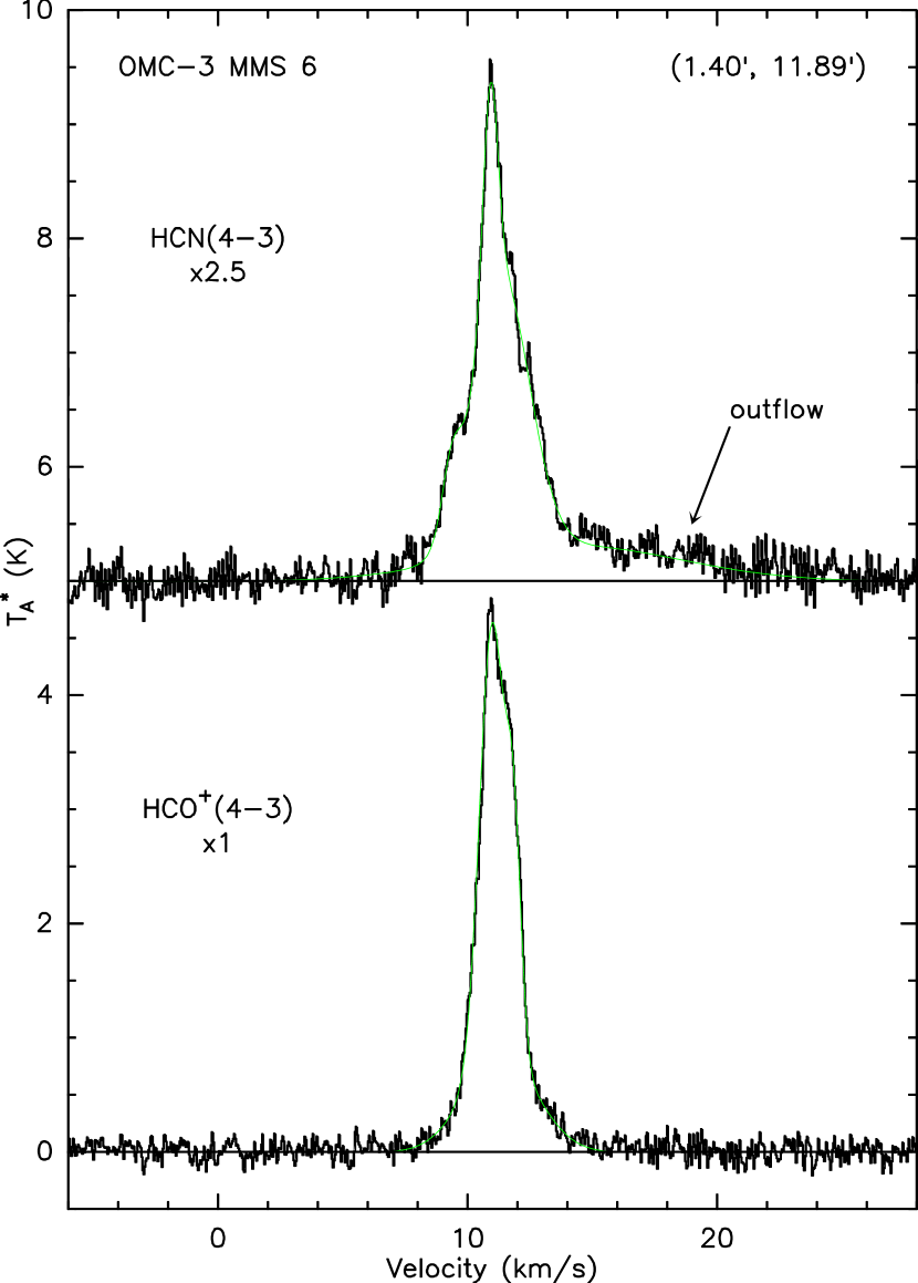
Figure 8: Spectra taken in OMC-3 MMS 6 that show the effect of a one-sided outflow on the evaluation of the HCO⁺/HCN line width ratio. The outflow is detected in HCN but not in HCO⁺. The line width ratio with and without accounting for the outflow is 0.34 and 0.87, respectively (see the text). The offset position from the reference at R.A.$=5^{h}32^{m}50^{s}$, decl.$=-5\arcdeg 15\arcmin 00\arcsec$ (B1950) (see Figure 10) is given in the upper right corner, in arcminutes.

In evaluating the line widths of the HCN and HCO⁺ spectra and, subsequently, their ratio care must be taken that the spectra studied are obtained in region suitable to this type of analysis. For example, the line width calculations and the models proposed by Houde et al. (2002) (see their equations (9) and (10) and Figure 2) make certain assumptions concerning the distribution of the neutral flows in velocity space. One consequence is that, ideally, the spectra should be even around the mean velocity. Although this will rarely be the case in turbulent molecular clouds, one should be careful that the departures from this idealization are not extreme. Such an example is shown in Figure 8 where we show a pair of HCN and HCO⁺ spectra taken in the OMC-3 MMS 6 region. We can see the clear signature of a one-sided outflow in the neutral line profile that is, however, missing from the ion spectrum. Although the presence of unresolved (bipolar) outflows within the telescope beam is not un-welcome when trying to calculate the orientation of the magnetic field, it does not make sense, for example, to discuss differences between line widths of coexistent neutral and ion species within a resolved outflow. The most that one can do in such cases is to look for similarities or differences in the line profiles and draw appropriate conclusions from them (Houde et al., 2001). For the case at hand, the inclusion of the outflow in the line width calculations brings an artificial reduction in the value of the line width ratio. More precisely, we have found two more positions of similar occurrences in OMC-3 MMS 6 (none in the other sources) where the presence of the one-sided outflow lowers the local HCO⁺ to HCN line width ratio and brings the corresponding mean inclination angle to $82.2^{\circ}$. In analyzing the data presented in the previous section, we have carefully removed the effect of the outflow, after fitting the spectra with Gaussian profiles, to ensure that we are within confines relevant to the model of Houde et al. (2002). After doing so, for the example shown in Figure 8, the line width ratio jumped from 0.34 to 0.87. This new ratio is very similar to that obtained in OMC-3 MMS 9, a region which exhibits line profiles that are alike to those found for OMC-3 MMS 6 when no outflows are present (see Figure 5). Moreover, it is seen that this apparently significant change has a relatively mild effect on the value of the inclination angle; as stated before, the latter has a revised value of $72.6^{\circ}$. This is not surprising considering the fact that the field appears to lie close to the plane of the sky where $\alpha$ is quite insensitive to such changes. No matter which value for the ratio is used, the conclusion is still that the field is severely inclined in relation to the line of sight.

3.3.4 An early assessment of our $\alpha$-measuring technique

Without the existence of an independent method for measuring the inclination angle of the magnetic field, it is difficult to determine the level of success attained using our technique. It is, however, possible to get an early assessment on its viability by combining the data presented in this paper with the earlier set for M17 published by Houde et al. (2002). Since M17 exhibits relatively low polarization levels ($\lesssim 4\%$) while Orion A (more precisely OMC-1) covers a range that goes as high as $\approx 10\%$, a combination of both sets of data will allow us to see how well our technique performs over a large range of polarization levels. Despite the strong depolarization observed in regions of higher flux, measurements obtained on the edges of the clouds where we find the most significant levels of polarization, should trace differences in the inclination angle from one cloud to the other.

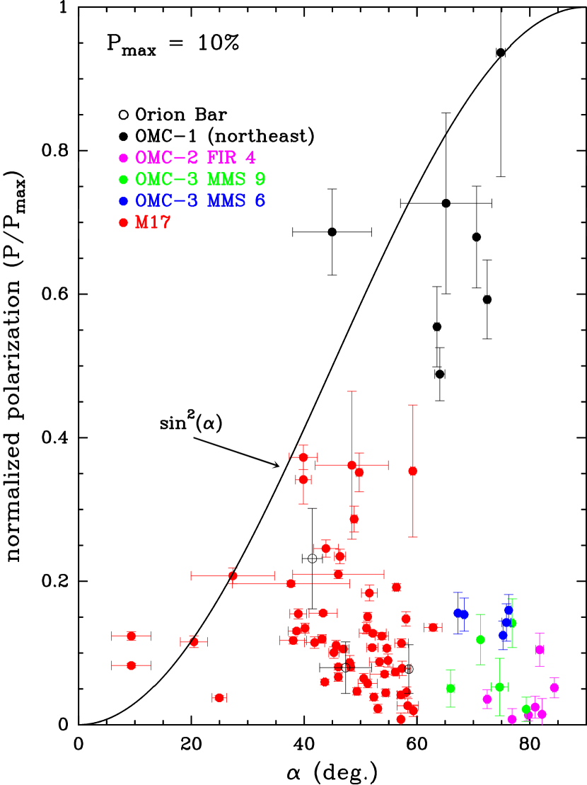
Figure 9: Normalized polarization level ($P/P_{max}$) vs the inclination angle ($\alpha$) for every source studied so far. The theoretical relation between the two parameters is also shown (solid curve). There is a good correspondence of low (high) polarization levels to small (large) inclination angles as would be expected.

We produced in Figure 9 a graph of the combined sets of data with the normalized polarization level plotted against the inclination angle. Also shown is a theoretical curve relating the two parameters (as would be the case in the absence of depolarization). As can be seen, there is a good correspondence between low (high) polarization levels and small (large) inclination angles. The polarization data for M17 are confined to a range where $\alpha\lesssim 60^{\circ}$ whereas the Orion A data set mostly covers $\alpha\gtrsim 60^{\circ}$, with most points being pushed down “under” the curve via the depolarization effect. Moreover, only three data points are located to the left of the theoretical curve. This is a good indication that the vast majority of pairs of polarization/line-width-ratio measurements fall within a domain that is predicted by our technique. Indications to the contrary could imply some shortcomings in our model and cast doubts on its adequacy. The results obtained so far are consistent with expectations.

4 Discussion

The results presented in Table 1 give us a glimpse into the orientation of the magnetic field in Orion A and can form the basis for an interpretation of its interaction with its environment. A few characteristics are easily noticeable upon studying Table 1. First, the inclination of the magnetic field varies little as one proceeds north to south along the ISF, this is especially true north of OMC-1. Second, the orientation of the magnetic field in the plane of the sky also shows little variations north of OMC-1 while it significantly changes direction at and within this high mass cloud. On the other hand, the orientation of the filament varies by some $60^{\circ}$ in the OMC-3 region alone, and by $\approx 80^{\circ}$ overall.

While it is true that in some parts (i.e., IRAS 05327-457, OMC-3 MMS 1-6 and north of OMC-2 FIR 3) the projection of the magnetic field is almost perpendicular to the local filament, and though this could be significant in itself (Matthews, Wilson & Fiege, 2001), we cannot say that there is a systematic trend for this. Similarly, there does not seem to exist a tendency for alignment as this is observed only in OMC-2 FIR 6 (see the last column of Table 1). Future polarimetry measurements which could fill the gaps in our coverage might, however, alter this picture. But for the present, it is perhaps more important to note that the absolute orientation of the sky-projected magnetic field changes by a relatively small amount over a large extent. In fact, from our data we see only one region north of OMC-1 (OMC-2 FIR 3) where there is an important deviation in the value of $\beta$ as compared to the other regions observed in OMC-3 and OMC-2. Neglecting OMC-2 FIR 3, we find that $\beta$ diminishes smoothly as one goes southward from IRAS 05327-457 to OMC-2 FIR 6, covering values ranging from $\approx 50^{\circ}$ to $\approx 25^{\circ}$. It is only when we reach the vicinity of the high mass star-forming region of OMC-1 that the orientation of the field varies considerably.

We could interpret these results as being consistent with a picture where the magnetic field is relatively unaffected by the presence of the concentrations of lower mass that characterize the OMC-3 and OMC-2 fields (Figures 1 and 2), adopting there an orientation similar to that which it may have on the larger scale. This aspect of the orientation of the magnetic field in connection to the larger scale will be treated in an upcoming paper by Poidevin and Bastien (in preparation). Moreover, the small changes in the inclination of the magnetic field to the line of sight in these parts of Orion A only reinforces the idea of a relatively unaffected magnetic field. The only significant variations in the value of $\alpha$ happen in OMC-1 (northeast) and in the Bar where it decreases to $\simeq 65^{\circ}$ and $\simeq 49^{\circ}$, respectively, from $\simeq 80^{\circ}$ in OMC-2 FIR 4. This is also accompanied by significant changes in $\beta$. This, in itself is not surprising for one would expect the magnetic field to be strongly perturbed by the presence of the large concentrations of mass found within OMC-1 and the greater amount of recent star formation in this region. The radiation and strong stellar winds emanating from the stars of the Trapezium must also affect the local magnetic field through their impact on the ionization fraction. The orientation of the magnetic field is indicated for five different positions along the ISF on the SHARC II map of Figure 10.

Finally, OMC-1 is one of the few clouds where there exists a Zeeman detection in CN. Crutcher (1999) reported a line-of-sight magnetic field strength of 360 $\mu$G at a position $\Delta\alpha\approx 10\arcsec$, $\Delta\delta\approx 20\arcsec$ away from IRc 2. If we assume that our value of $\alpha\simeq 65^{\circ}$ obtained in OMC-1 (northeast) applies equally well at this location, we calculate a magnitude of $\approx 850\,\,\mu$G for the magnetic field. This is not too far from that which was used by Crutcher (1999), based on statistical arguments, and therefore corroborates the conclusions reached there. More precisely, OMC-1 is magnetically supercritical with a mass-to-flux ratio $M/\Phi_{B}\approx 2.6$, and magnetic-to-gravitational and kinetic-to-gravitational energy ratios of $\approx 0.26$ and $\approx 0.30$, respectively. The combination of the magnetic and internal motion energies can therefore provide a significant amount of support against gravitation.

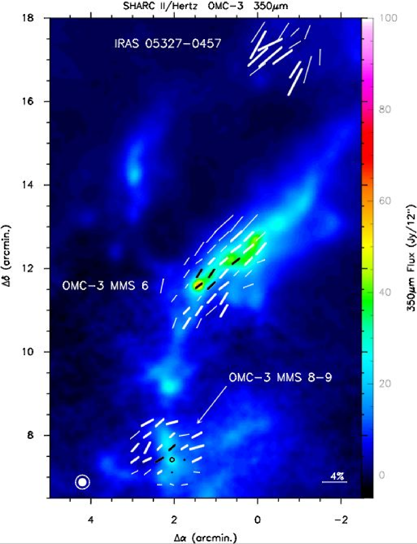
Figure 1: 350 $\mu$m continuum map and polarimetry (E-vectors) of the OMC-3 region obtained with SHARC II and Hertz, respectively. The thick (thin) vectors have a polarization level and uncertainty such that $P\geq 3\sigma_{P}$ ($P\geq 2\sigma_{P}$). The circle indicates a case where $P+2\sigma_{P}<1\%$ and $P<2\sigma_{P}$. The darker polarization vectors, circle, and dots denote positions where spectroscopic data were obtained. The beam widths are shown in the lower left corner, with the solid and open circles for SHARC II at $\simeq 12\arcsec$ and Hertz at $\simeq 20\arcsec$, respectively. The reference position is at R.A.$=5^{h}32^{m}50^{s}$, decl.$=-5\arcdeg 15\arcmin 00\arcsec$ (B1950).

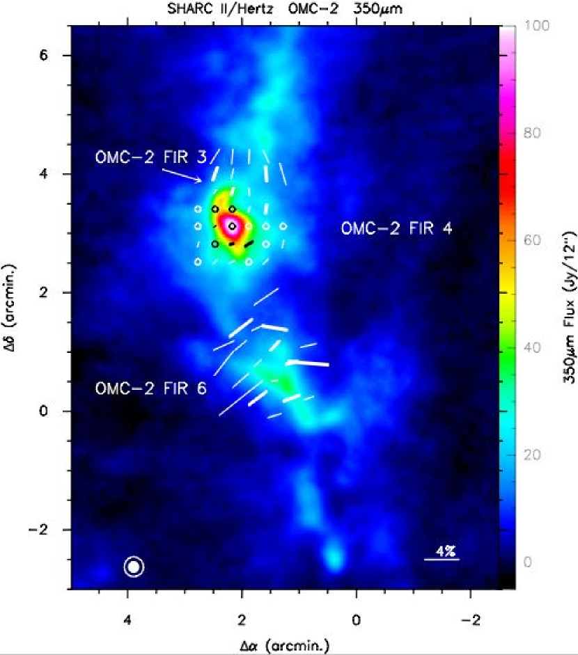
Figure 2: 350 $\mu$m continuum map and polarimetry (E-vectors) of the OMC-2 region obtained with SHARC II and Hertz, respectively. The thick (thin) vectors have a polarization level and uncertainty such that $P\geq 3\sigma_{P}$ ($P\geq 2\sigma_{P}$). Circles indicate cases where $P+2\sigma_{P}<1\%$ and $P<2\sigma_{P}$. The darker polarization vectors and circles denote positions where spectroscopic data were also obtained. The beam widths are shown in the lower left corner, with the solid and open circles for SHARC II at $\simeq 12\arcsec$ and Hertz at $\simeq 20\arcsec$, respectively. The reference position is at R.A.$=5^{h}32^{m}50^{s}$, decl.$=-5\arcdeg 15\arcmin 00\arcsec$ (B1950).

Figure 6: The polarization level vs the 350 $\mu$m continuum flux for the polarimetry data as shown for the OMC-3 and OMC-2 fields of Figures 1 and 2, respectively, where $P\geq 2\sigma_{P}$. The depolarization effect is clearly seen.

Table 1: Results - Orientation of the magnetic field in Orion A

Object	$\alpha$	$\sigma_{\alpha}$	$\beta$	$\sigma_{\beta}$	$\gamma$	$\mid\beta-\gamma\mid$
IRAS 05327-457	$\cdots$	$\cdots$	$52.6^{\circ}$	$3.0^{\circ}$	$\sim 132^{\circ}$	$\sim 79^{\circ}$
OMC-3 MMS 6	$72.6^{\circ}$	$4.4^{\circ}$	$46.3^{\circ}$	$1.0^{\circ}$	$\sim 132^{\circ}$	$\sim 86^{\circ}$
OMC-3 MMS 9	$73.7^{\circ}$	$5.2^{\circ}$	$38.5^{\circ}$	$2.8^{\circ}$	$\sim 8^{\circ}$	$\sim 31^{\circ}$
OMC-2 FIR 3	$\cdots$	$\cdots$	$84.6^{\circ}$	$3.8^{\circ}$	$\sim 160^{\circ}$	$\sim 75^{\circ}$
OMC-2 FIR 4	$79.8^{\circ}$	$4.0^{\circ}$	$31.3^{\circ}$	$4.6^{\circ}$	$\sim 0^{\circ}$	$\sim 31^{\circ}$
OMC-2 FIR 6	$\cdots$	$\cdots$	$25.0^{\circ}$	$6.2^{\circ}$	$\sim 35^{\circ}$	$\sim 10^{\circ}$
OMC-1 (northeast)	$65.1^{\circ}$	$9.9^{\circ}$	$130.2^{\circ}$	$0.3^{\circ}$	$\sim 10^{\circ}$	$\sim 120^{\circ}$
Bar	$49.1^{\circ}$	$8.7^{\circ}$	$81.8^{\circ}$	$3.6^{\circ}$	$\sim 52^{\circ}$	$\sim 30^{\circ}$
OMC-4	$\cdots$	$\cdots$	$73.7^{\circ}$	$2.8^{\circ}$	$\sim 25^{\circ}$	$\sim 49^{\circ}$

Table 2: OMC-1, 350 µm Results

$\Delta\alpha$	$\Delta\delta$	$P$	$\sigma_{P}$	$PA$	$\sigma_{PA}$	Flux
-1.69	-13.85	10.17	5.02	133.6	14.1	54.2
-1.39	-13.85	4.08	1.40	143.9	9.7	79.7
-1.69	-13.56	5.09	2.06	147.1	11.4	54.2
-1.39	-13.56	2.33	1.08	125.4	13.3	80.4
-1.09	-13.56	2.04	0.47	148.3	6.7	115.7
-0.80	-13.56	1.11	0.29	154.8	7.5	139.8
-1.69	-13.26	4.22	1.11	146.2	6.4	57.9
-1.39	-13.26	2.18	0.47	147.2	6.0	79.6
-1.09	-13.26	1.22	0.33	157.4	7.8	109.9
-0.80	-13.26	1.09	0.17	139.7	4.1	141.6
-0.50	-13.26	0.82	0.22	120.8	7.6	134.1
-0.20	-13.26	0.22	0.24	95.0	31.2	110.1
-1.98	-12.96	3.47	1.04	153.3	8.5	53.1
-1.69	-12.96	2.28	0.73	154.3	9.2	61.5
-1.39	-12.96	1.66	0.36	161.8	6.3	77.7
-1.09	-12.96	1.14	0.20	162.1	5.1	104.7
-0.80	-12.96	0.63	0.21	158.9	9.2	145.6
-0.50	-12.96	0.63	0.20	141.4	6.2	141.4
-0.20	-12.96	0.14	0.19	113.9	39.3	129.7
0.09	-12.96	0.33	0.23	56.8	20.1	106.0
-2.56	-12.92	6.17	2.15	163.2	10.1	29.8
-2.26	-12.92	4.03	1.77	155.0	12.6	37.4
-1.96	-12.92	5.25	1.11	154.2	6.1	53.5
-1.67	-12.92	3.94	0.74	143.9	5.4	76.7
-1.98	-12.67	3.19	1.04	155.8	9.4	52.6
-1.69	-12.67	2.06	0.66	157.1	9.2	71.3
-1.39	-12.67	1.78	0.32	151.9	5.2	80.7
-1.09	-12.67	1.60	0.21	161.1	3.7	97.4
-0.80	-12.67	1.24	0.14	168.3	3.4	133.8
-0.20	-12.67	0.96	0.33	2.3	5.9	133.5
-0.50	-12.67	0.90	0.15	179.2	4.0	142.6
0.09	-12.67	1.61	0.24	14.7	4.2	124.4
0.39	-12.67	2.18	0.36	16.7	4.7	110.8
-2.85	-12.62	6.09	2.55	156.3	12.0	26.9
-2.56	-12.62	6.13	1.22	173.5	5.9	36.4
-2.26	-12.62	4.38	0.91	165.5	6.0	46.5
-1.96	-12.62	2.98	0.59	149.0	5.8	67.9
-1.67	-12.62	1.51	0.49	145.8	9.5	92.1
-0.18	-12.62	1.54	0.76	41.4	15.1	161.9
-1.98	-12.37	2.71	0.68	148.0	7.0	65.2
-1.69	-12.37	1.77	0.44	152.4	7.2	81.9
-1.09	-12.37	0.65	0.20	152.4	8.8	115.1
-0.80	-12.37	0.40	0.17	157.3	12.7	131.6
-0.50	-12.37	0.77	0.15	7.4	5.5	138.4
-0.20	-12.37	1.15	0.22	20.4	5.4	141.0
0.09	-12.37	1.38	0.24	14.2	4.9	125.5
0.39	-12.37	1.41	0.33	5.0	6.7	114.8
0.71	-12.36	2.32	0.70	167.6	8.6	106.6
1.30	-12.36	0.88	0.37	115.5	12.1	87.9
1.60	-12.36	2.19	0.68	96.3	8.8	61.5
-2.85	-12.32	4.72	1.36	165.5	8.4	36.1
-2.56	-12.32	4.51	0.92	154.4	5.8	57.3
-2.26	-12.32	3.12	0.61	159.1	5.6	71.5
-1.96	-12.32	2.53	0.42	150.2	4.8	102.2
-1.67	-12.32	0.89	0.37	142.3	11.1	136.2
-1.37	-12.32	0.80	0.24	146.3	8.4	167.3
-0.78	-12.32	0.72	0.28	59.0	11.3	213.8
-0.48	-12.32	0.98	0.23	50.8	6.8	198.3
-0.18	-12.32	1.52	0.34	30.7	7.3	173.7
0.11	-12.32	1.42	0.62	41.2	9.2	139.7
1.00	-12.32	4.41	2.02	122.9	13.0	145.6
-1.98	-12.07	1.86	0.66	155.7	10.2	87.8
-1.69	-12.07	1.44	0.39	147.9	7.9	112.2
-1.09	-12.07	0.51	0.17	138.4	9.4	153.3
-0.80	-12.07	0.40	0.14	79.6	10.2	175.1
-0.50	-12.07	0.60	0.13	51.6	7.3	164.4
-0.20	-12.07	0.87	0.19	30.5	6.2	146.1
0.09	-12.07	0.71	0.25	40.5	9.9	131.3
0.39	-12.07	1.00	0.42	17.4	11.9	122.4
2.19	-12.07	2.42	0.82	97.6	9.6	49.1
1.30	-12.07	0.80	0.36	104.9	12.9	117.3
1.89	-12.07	1.97	0.55	77.9	8.0	66.4
-2.85	-12.03	3.51	0.97	177.3	8.0	58.3
-2.56	-12.03	3.65	0.99	166.9	6.1	69.7
-2.26	-12.03	2.72	0.44	162.3	4.6	89.2
-1.96	-12.03	1.65	0.39	160.0	7.2	133.2
-1.67	-12.03	0.62	0.19	167.8	9.0	200.7
-1.37	-12.03	0.01	0.15	115.9	452.5	244.7
-1.07	-12.03	0.65	0.25	150.6	13.8	285.8
-0.78	-12.03	0.77	0.17	38.5	5.6	310.5
-0.48	-12.03	1.47	0.21	43.7	3.2	249.4
-0.18	-12.03	1.33	0.19	40.3	4.1	188.5
0.11	-12.03	1.36	0.27	32.6	5.8	162.4
0.41	-12.03	2.17	0.47	36.5	6.1	120.6
0.71	-12.03	1.31	0.60	24.8	13.1	130.8
-1.98	-11.78	4.64	1.39	176.5	8.7	107.3
-1.69	-11.78	1.00	0.34	146.9	10.1	167.4
-1.39	-11.78	0.63	0.25	123.1	11.0	200.9
-1.09	-11.78	0.58	0.15	102.7	7.0	234.3
-0.80	-11.78	0.81	0.13	52.3	6.9	241.0
-0.50	-11.78	1.48	0.17	45.0	4.0	217.9
-0.20	-11.78	1.42	0.23	29.6	4.6	171.9
0.09	-11.78	1.41	0.39	44.1	7.9	147.6
0.71	-11.77	1.09	0.51	54.3	13.4	83.9
1.60	-11.77	0.78	0.34	85.2	12.4	108.5
1.89	-11.77	0.90	0.37	80.4	11.5	96.1
2.19	-11.77	1.16	0.50	96.9	12.4	67.3
-2.85	-11.73	3.56	0.68	3.1	5.3	75.7
-2.56	-11.73	2.67	0.56	165.7	6.0	88.8
-2.26	-11.73	2.19	0.38	165.2	4.9	107.2
-1.96	-11.73	0.92	0.25	177.8	7.9	154.3
-1.67	-11.73	0.72	0.17	169.6	6.6	232.7
-1.37	-11.73	0.35	0.13	175.6	11.7	342.5
-1.07	-11.73	0.32	0.10	45.1	9.5	506.3
-0.78	-11.73	1.02	0.08	45.0	2.4	524.8
-0.48	-11.73	1.70	0.16	43.7	3.3	325.7
-0.18	-11.73	1.76	0.15	43.8	2.4	234.9
0.11	-11.73	1.99	0.21	32.0	3.0	189.6
0.41	-11.73	1.99	0.30	42.3	4.3	141.8
0.71	-11.73	1.46	0.46	41.4	9.1	120.0
-1.39	-11.48	0.61	0.30	86.7	14.5	319.4
-1.09	-11.48	0.42	0.21	84.5	14.5	422.2
-0.80	-11.48	1.22	0.21	60.9	4.9	432.3
0.71	-11.47	2.97	0.90	34.2	8.9	74.2
1.00	-11.47	0.90	0.45	46.1	14.3	73.1
1.30	-11.47	1.54	0.44	51.5	8.2	80.8
1.89	-11.47	1.51	0.29	110.4	5.6	118.6
-2.85	-11.43	3.00	1.04	175.9	6.6	83.4
-2.56	-11.43	1.13	0.44	176.8	11.2	98.1
-2.26	-11.43	2.15	0.44	169.5	4.6	131.4
-1.96	-11.43	0.89	0.20	173.2	9.4	182.0
-1.67	-11.43	1.16	0.12	11.3	3.1	257.0
-1.37	-11.43	0.80	0.12	9.8	4.5	411.1
-1.07	-11.43	0.97	0.07	23.7	2.2	886.1
-0.78	-11.43	1.13	0.11	29.7	1.9	952.8
-0.48	-11.43	1.67	0.14	37.3	2.0	466.0
-0.18	-11.43	2.18	0.18	38.9	1.7	285.6
0.11	-11.43	2.32	0.17	39.6	2.2	213.3
0.41	-11.43	1.88	0.25	33.6	3.7	159.0
0.71	-11.43	1.17	0.45	33.9	10.9	127.5
1.00	-11.43	1.65	0.68	46.5	11.8	127.7
1.89	-11.18	1.26	0.47	64.0	10.7	89.9
-2.85	-11.14	3.14	0.94	175.5	8.6	93.6
-2.56	-11.14	3.00	0.85	166.6	5.8	107.8
-2.26	-11.14	2.68	0.33	173.9	3.5	153.1
-1.96	-11.14	1.58	0.21	177.5	3.9	220.5
-1.67	-11.14	1.17	0.15	13.3	3.9	316.0
-1.37	-11.14	1.23	0.24	20.8	5.1	442.0
-1.07	-11.14	1.76	0.07	24.2	1.1	766.0
-0.78	-11.14	2.04	0.11	24.0	1.4	947.8
-0.48	-11.14	2.57	0.10	27.7	1.0	491.0
-0.18	-11.14	2.78	0.12	29.2	1.3	308.0
0.11	-11.14	2.25	0.19	26.8	2.5	222.6
0.41	-11.14	2.40	0.28	29.4	3.3	157.8
0.71	-11.14	1.54	0.45	38.1	8.8	118.4
1.00	-11.14	1.49	0.56	32.7	10.9	133.8
-2.56	-10.84	2.97	0.63	0.2	6.1	135.7
-2.26	-10.84	1.43	0.39	5.0	7.8	190.1
-1.96	-10.84	2.01	0.27	22.5	3.9	270.5
-1.67	-10.84	2.13	0.23	14.3	3.1	351.8
-1.37	-10.84	1.61	0.25	25.2	4.9	477.7
-1.07	-10.84	2.64	0.17	24.3	1.7	657.5
-0.78	-10.84	2.82	0.10	25.5	1.0	709.0
-0.48	-10.84	2.71	0.10	26.8	1.1	450.6
-0.18	-10.84	2.96	0.12	25.5	1.2	349.8
0.11	-10.84	2.44	0.17	29.2	2.0	232.6
0.41	-10.84	2.25	0.30	20.1	3.8	160.1
0.71	-10.84	2.63	0.50	15.2	5.4	120.8
1.00	-10.84	2.52	0.70	13.5	8.2	126.5
-1.05	-10.60	1.51	0.15	37.6	2.9	832.2
-0.75	-10.60	1.91	0.17	17.9	2.5	988.7
-0.45	-10.60	2.47	0.37	26.2	4.3	400.0
-0.16	-10.60	2.13	0.35	18.5	4.7	276.3
-2.56	-10.54	2.13	0.70	20.2	9.5	160.8
-2.26	-10.54	2.26	0.58	8.6	7.4	194.2
-1.96	-10.54	1.60	0.42	12.7	7.5	280.4
-1.67	-10.54	1.90	0.38	32.6	5.7	444.7
-1.07	-10.54	3.44	0.31	21.5	2.6	547.2
-0.78	-10.54	3.54	0.22	22.8	1.8	573.2
-0.48	-10.54	3.24	0.17	26.6	1.5	449.9
-0.18	-10.54	3.05	0.19	25.3	1.7	368.8
0.11	-10.54	2.84	0.21	28.2	2.1	273.7
0.41	-10.54	3.07	0.39	21.3	3.6	183.4
0.71	-10.54	2.38	0.61	26.2	7.3	198.2
1.30	-10.54	2.74	1.13	170.5	11.1	125.4
-2.53	-10.31	2.32	0.58	10.0	7.1	132.6
-2.23	-10.31	1.91	0.48	20.3	7.1	169.8
-1.94	-10.31	2.12	0.33	18.2	4.4	232.9
-1.64	-10.31	2.79	0.25	19.5	2.5	291.5
-1.34	-10.31	1.89	0.08	24.1	1.2	531.5
-1.05	-10.31	3.07	0.08	27.3	0.9	665.4
-0.75	-10.31	3.33	0.07	26.4	0.6	647.1
-0.45	-10.31	3.02	0.05	26.4	0.5	460.2
-0.16	-10.31	2.50	0.09	28.0	1.1	341.8
0.14	-10.31	2.12	0.47	21.9	6.3	236.3
0.11	-10.25	2.20	0.37	27.9	4.9	331.0
0.41	-10.25	3.12	0.79	32.6	7.3	245.8
0.71	-10.25	2.51	0.66	38.7	7.6	220.7
1.00	-10.25	1.81	0.89	33.0	14.7	165.2
-2.83	-10.01	2.12	0.52	10.6	7.0	141.9
-2.53	-10.01	2.22	0.30	14.8	3.8	178.3
-2.23	-10.01	2.11	0.25	21.9	3.4	200.8
-1.94	-10.01	2.62	0.21	28.6	2.4	249.9
-1.64	-10.01	2.54	0.07	22.0	0.8	406.7
-1.34	-10.01	2.57	0.04	27.6	0.5	531.7
-1.05	-10.01	2.98	0.05	27.7	0.5	788.2
-0.75	-10.01	3.45	0.07	26.2	0.6	708.0
-0.45	-10.01	2.97	0.06	27.6	0.5	535.2
-0.16	-10.01	2.60	0.05	23.8	0.5	377.8
0.14	-10.01	2.37	0.14	23.1	1.7	279.3
-2.83	-9.71	2.55	0.34	24.1	3.8	154.8
-2.53	-9.71	2.52	0.30	23.4	3.4	174.1
-2.23	-9.71	2.70	0.26	23.3	2.7	196.7
-1.94	-9.71	2.67	0.18	28.8	1.9	226.8
-1.64	-9.71	2.76	0.07	28.2	0.7	358.5
-1.34	-9.71	2.77	0.06	29.1	0.5	538.5
-1.05	-9.71	2.50	0.06	26.8	0.7	999.4
-0.75	-9.71	2.01	0.04	31.0	0.6	1257.8
-0.45	-9.71	2.41	0.07	26.3	0.8	697.9
-0.16	-9.71	2.53	0.04	22.2	0.5	423.3
0.14	-9.71	2.47	0.08	23.0	0.9	296.5
0.44	-9.71	2.67	0.26	20.0	2.8	215.7
0.73	-9.71	2.87	0.37	10.1	3.5	164.1
1.03	-9.71	2.60	0.46	11.4	5.0	102.8
1.33	-9.71	2.76	0.55	6.6	5.4	82.3
-1.94	-9.42	3.00	0.18	32.7	1.7	237.0
0.44	-9.42	2.51	0.18	17.7	2.1	235.6
-0.75	-9.42	1.06	0.04	33.3	1.3	2100.0
-2.83	-9.42	2.30	0.47	42.1	5.8	118.4
-2.53	-9.42	2.97	0.36	36.7	3.5	138.9
-2.23	-9.42	2.26	0.35	32.7	4.5	159.6
-1.64	-9.42	2.91	0.05	32.9	0.5	399.5
-1.34	-9.42	2.88	0.04	32.4	0.5	531.7
-1.05	-9.42	2.10	0.06	28.5	0.6	1011.5
-0.45	-9.42	1.89	0.04	24.5	0.6	952.9
-0.16	-9.42	2.67	0.06	19.4	0.6	473.5
0.14	-9.42	2.46	0.12	17.5	1.1	316.0
0.73	-9.42	2.81	0.31	8.6	3.1	158.7
1.03	-9.42	2.80	0.37	3.5	3.7	111.1
1.33	-9.42	2.66	0.49	2.1	5.2	94.6
1.62	-9.42	3.27	0.54	176.7	4.8	81.9
-2.83	-9.12	3.20	0.57	44.3	5.1	106.2
-2.53	-9.12	3.22	0.42	33.2	3.7	131.5
-2.23	-9.12	2.85	0.30	34.9	2.9	172.5
-1.94	-9.12	2.78	0.17	34.8	1.8	267.1
-1.64	-9.12	2.74	0.05	37.5	0.9	387.6
-1.34	-9.12	2.38	0.05	37.0	0.8	516.0
-1.05	-9.12	2.02	0.04	35.1	0.5	807.4
-0.75	-9.12	1.49	0.05	34.0	1.1	1238.4
-0.45	-9.12	2.33	0.05	22.6	0.6	1134.4
-0.16	-9.12	2.88	0.05	14.1	0.4	508.9
0.14	-9.12	2.52	0.07	13.1	0.9	311.7
0.44	-9.12	2.34	0.22	8.3	4.7	231.2
0.73	-9.12	2.77	0.29	178.7	3.0	156.0
1.03	-9.12	3.05	0.38	2.0	3.6	127.1
1.33	-9.12	2.45	0.44	7.6	4.9	103.7
1.62	-9.12	2.58	0.56	2.5	6.1	82.1
-2.83	-8.82	3.02	0.82	35.1	7.8	103.3
-2.53	-8.82	3.58	0.40	39.7	3.2	144.0
-2.23	-8.82	3.41	0.29	37.4	2.5	174.9
-1.94	-8.82	2.96	0.19	42.3	1.9	236.1
-1.64	-8.82	2.80	0.11	39.6	0.9	342.1
-1.34	-8.82	2.28	0.04	40.1	0.6	455.7
-1.05	-8.82	1.94	0.03	39.0	0.7	615.0
-0.75	-8.82	2.07	0.05	38.3	0.6	725.1
-0.45	-8.82	1.79	0.04	29.1	0.8	949.0
-0.16	-8.82	2.20	0.05	13.0	0.6	552.6
0.14	-8.82	2.65	0.07	10.5	0.8	316.5
0.44	-8.82	2.37	0.17	4.3	2.1	243.6
0.73	-8.82	4.03	0.59	4.6	4.2	184.9
1.03	-8.82	3.52	0.40	1.6	3.2	151.1
1.33	-8.82	3.59	0.47	3.1	3.6	115.2
1.62	-8.82	5.65	0.70	1.1	3.5	83.8
-2.53	-8.53	4.10	0.60	39.9	4.1	157.4
-2.23	-8.53	3.34	0.60	35.3	5.2	148.4
-1.94	-8.53	3.62	0.32	43.7	2.6	193.3
-1.64	-8.53	3.37	0.28	37.8	2.4	265.5
-1.34	-8.53	2.32	0.09	45.1	1.1	381.8
-1.05	-8.53	2.19	0.06	41.5	0.7	467.0
-0.75	-8.53	2.18	0.07	36.3	0.6	508.9
-0.45	-8.53	1.86	0.04	28.2	0.8	566.1
-0.16	-8.53	1.76	0.06	15.4	1.0	482.0
0.14	-8.53	1.96	0.10	10.6	1.9	437.9
0.44	-8.53	2.34	0.18	178.7	3.1	268.5
0.73	-8.53	2.52	0.28	178.0	3.2	194.9
1.03	-8.53	3.01	0.33	179.2	3.2	152.6
1.33	-8.53	4.30	0.69	176.5	4.7	111.4
1.62	-8.53	4.61	0.71	177.4	4.4	80.0
-2.62	-8.41	2.39	0.82	57.7	9.9	109.7
-2.32	-8.41	3.16	0.81	48.7	7.2	119.1
-2.03	-8.41	5.66	0.63	50.0	3.1	146.1
-1.73	-8.41	4.43	0.47	50.1	3.0	187.9
-0.84	-8.40	2.20	0.22	39.4	2.9	408.3
-0.55	-8.40	1.93	0.14	33.9	2.1	489.2
-0.25	-8.40	1.57	0.13	21.3	2.4	542.8
0.05	-8.40	1.47	0.14	17.6	2.7	496.2
0.34	-8.40	1.68	0.22	5.0	3.8	411.2
0.64	-8.40	3.17	0.28	177.1	2.6	212.4
0.94	-8.40	4.04	0.49	175.7	3.5	155.4
1.23	-8.40	3.35	0.55	5.2	4.8	102.9
1.53	-8.40	5.43	0.86	1.6	4.5	67.0
-1.64	-8.23	3.82	0.79	45.9	5.9	191.9
-1.34	-8.23	3.41	0.66	46.3	5.5	217.2
-1.05	-8.23	2.36	0.21	43.6	2.6	320.3
-0.75	-8.23	2.01	0.15	41.1	2.0	399.4
-0.45	-8.23	1.61	0.13	28.0	2.2	541.4
-0.16	-8.23	1.87	0.15	19.6	2.4	470.5
0.14	-8.23	1.60	0.23	23.3	4.2	415.8
0.44	-8.23	1.63	0.26	174.5	4.7	286.0
0.73	-8.23	3.25	0.35	175.5	3.1	183.3
1.03	-8.23	3.35	0.45	178.0	3.9	134.7
1.33	-8.23	3.04	0.50	179.1	4.7	103.6
-2.92	-8.11	6.01	1.51	59.9	7.0	73.1
-2.62	-8.11	3.18	0.95	50.5	8.2	94.0
-2.32	-8.11	2.78	0.73	53.1	7.3	103.8
-2.03	-8.11	4.59	0.59	48.3	3.6	138.3
-1.73	-8.11	3.86	0.45	49.8	3.3	181.1
-1.43	-8.11	3.10	0.46	44.5	4.3	185.2
-1.14	-8.10	2.45	0.35	47.4	4.0	293.4
-0.84	-8.10	2.06	0.11	40.8	1.5	350.5
-0.55	-8.10	1.89	0.07	35.3	1.0	488.3
-0.25	-8.10	1.68	0.07	20.8	1.2	483.9
0.05	-8.10	1.42	0.09	13.7	1.8	341.5
0.34	-8.10	1.29	0.32	5.3	2.8	337.9
0.64	-8.10	1.71	0.22	179.8	4.9	257.1
0.94	-8.10	3.21	0.38	176.6	3.4	152.3
1.23	-8.10	4.29	0.60	176.3	4.0	103.1
1.53	-8.10	6.54	0.97	178.7	4.3	75.1
1.83	-8.10	5.72	1.34	5.0	6.4	53.4
-2.92	-7.81	5.35	1.69	70.3	9.0	59.8
-2.62	-7.81	3.94	1.11	44.2	8.1	71.4
-2.32	-7.81	2.66	1.10	52.2	11.5	92.0
-2.03	-7.81	3.89	0.63	49.6	4.5	126.0
-1.73	-7.81	2.47	0.48	46.2	5.5	161.3
-1.43	-7.81	3.99	0.48	48.5	3.4	168.6
-1.14	-7.81	2.63	0.17	48.9	1.8	255.4
-0.84	-7.81	1.96	0.10	47.3	1.4	286.9
-0.55	-7.81	1.58	0.07	41.1	1.3	393.6
-0.25	-7.81	1.22	0.05	20.4	1.2	493.1
0.05	-7.81	1.28	0.08	18.1	1.7	357.1
0.34	-7.81	1.23	0.20	14.9	3.1	293.6
0.64	-7.81	1.69	0.16	7.6	3.3	205.4
0.94	-7.81	2.61	0.31	2.4	3.4	145.8
1.23	-7.81	3.18	0.42	6.8	3.7	102.1
1.53	-7.81	4.53	0.57	9.3	3.4	79.9
1.83	-7.81	6.60	1.03	15.7	4.4	63.1
2.12	-7.81	5.48	2.34	175.8	12.2	61.4
-2.92	-7.52	5.87	1.87	51.4	8.7	48.0
-2.62	-7.52	3.65	1.60	66.3	12.6	59.8
-2.03	-7.52	4.31	0.66	53.6	4.2	126.8
-1.73	-7.52	3.89	0.58	52.3	4.1	146.0
-1.43	-7.52	3.23	0.60	68.5	5.3	147.5
-2.32	-7.52	3.48	1.02	54.6	8.2	82.8
-1.14	-7.51	2.06	0.19	55.3	2.6	219.2
-0.84	-7.51	1.64	0.12	50.4	2.0	260.3
-0.55	-7.51	1.36	0.07	41.5	1.4	420.6
-0.25	-7.51	0.68	0.06	31.5	2.4	483.3
0.05	-7.51	0.79	0.07	23.5	2.6	341.3
0.34	-7.51	1.36	0.10	14.9	2.9	288.4
0.64	-7.51	1.77	0.15	13.0	2.4	205.4
0.94	-7.51	3.02	0.43	17.3	4.1	131.0
1.23	-7.51	3.72	0.58	11.8	3.2	107.0
1.53	-7.51	5.74	0.50	14.8	2.4	89.1
1.83	-7.51	6.87	0.60	12.8	2.4	78.9
2.12	-7.51	7.59	1.49	18.2	5.6	80.4
2.42	-7.51	7.87	2.05	19.1	7.5	79.0
-2.92	-7.22	8.08	3.53	64.2	12.5	40.0
-2.62	-7.22	2.88	1.15	50.2	11.4	54.3
-2.32	-7.22	3.67	0.81	53.2	6.4	80.7
-2.03	-7.22	2.55	0.40	47.5	4.5	120.9
-1.73	-7.22	3.57	0.63	57.0	4.7	112.6
-1.43	-7.22	4.31	1.12	62.1	7.4	126.9
-1.14	-7.21	2.41	0.24	55.1	2.8	183.7
-0.84	-7.21	1.79	0.11	50.1	1.7	228.6
-0.55	-7.21	1.74	0.07	35.8	1.1	342.3
-0.25	-7.21	1.12	0.06	36.4	1.6	346.8
0.05	-7.21	0.94	0.08	42.4	2.4	261.7
0.34	-7.21	1.45	0.10	27.6	2.1	241.8
0.64	-7.21	2.34	0.17	20.9	2.0	192.9
0.94	-7.21	3.85	0.32	20.4	2.4	141.9
1.23	-7.21	4.20	0.43	20.2	2.9	114.7
1.53	-7.21	5.55	0.56	17.4	2.9	107.3
1.83	-7.21	5.25	0.44	13.4	2.4	105.4
2.12	-7.21	6.23	1.04	18.5	4.8	104.4
2.42	-7.21	5.79	1.44	6.2	7.0	75.9
-2.62	-6.92	3.12	1.19	48.5	11.0	50.5
-2.32	-6.92	3.63	0.79	47.2	5.6	77.9
-2.03	-6.92	3.94	0.46	57.0	3.4	104.5
-1.73	-6.92	3.57	0.58	64.3	4.6	99.0
-1.43	-6.92	2.64	0.77	46.8	8.5	107.3
-0.84	-6.92	2.31	0.11	51.7	1.3	205.3
-0.55	-6.92	1.86	0.07	41.8	1.1	302.4
0.05	-6.92	1.47	0.09	37.7	1.7	227.0
0.34	-6.92	2.24	0.10	32.8	1.2	208.2
0.64	-6.92	3.15	0.16	31.0	1.3	189.4
0.94	-6.92	4.26	0.33	34.7	3.1	150.6
1.23	-6.92	4.89	0.37	21.4	2.2	116.7
1.53	-6.92	5.75	0.48	17.5	2.4	104.2
1.83	-6.92	6.80	0.71	21.5	3.0	95.6
2.12	-6.92	7.27	1.26	13.7	4.9	82.4
2.42	-6.92	9.37	1.73	8.5	5.1	64.9
-0.25	-6.92	1.28	0.07	37.0	1.5	304.8
-1.14	-6.92	2.84	0.19	54.6	1.9	157.0
-2.62	-6.63	3.92	1.39	41.6	9.9	46.0
-2.32	-6.63	4.33	0.93	50.2	6.2	65.5
-2.03	-6.63	3.43	0.72	57.8	5.9	77.5
-1.73	-6.63	2.88	0.73	44.3	7.3	86.3
-1.43	-6.63	4.21	0.84	53.1	5.6	94.2
-1.14	-6.62	3.71	0.28	48.9	2.2	150.3
-0.84	-6.62	2.33	0.14	53.3	1.7	194.2
-0.55	-6.62	1.83	0.08	44.5	1.3	268.5
-0.25	-6.62	1.39	0.06	41.6	1.2	342.2
0.05	-6.62	1.96	0.08	39.0	1.2	235.7
0.34	-6.62	2.64	0.10	33.0	1.1	200.9
0.64	-6.62	3.64	0.24	33.8	1.5	172.1
0.94	-6.62	4.56	0.28	30.2	1.8	154.8
1.23	-6.62	5.93	0.55	23.8	2.7	115.1
1.53	-6.62	5.13	0.94	22.3	5.2	96.5
1.83	-6.62	4.93	0.90	13.5	6.1	75.2
2.12	-6.62	5.48	1.78	3.4	9.2	57.2
2.42	-6.62	5.69	2.38	11.9	11.6	45.5
-2.62	-6.33	4.39	1.81	49.9	11.7	43.3
-2.32	-6.33	2.73	1.05	61.2	11.0	55.9
-2.03	-6.33	3.98	0.92	44.9	6.6	66.7
-1.73	-6.33	4.16	0.83	51.7	5.6	78.1
-1.43	-6.33	3.78	1.09	52.5	8.2	92.4
-1.14	-6.32	3.40	0.31	55.8	2.5	148.0
-0.84	-6.32	2.45	0.16	49.8	1.8	200.2
-0.55	-6.32	1.56	0.09	48.8	1.7	278.9
-0.25	-6.32	1.62	0.06	45.0	1.1	395.0
0.05	-6.32	1.88	0.07	41.6	1.0	311.9
0.34	-6.32	2.98	0.13	35.3	1.2	199.5
0.64	-6.32	3.87	0.18	32.0	1.3	157.3
0.94	-6.32	4.80	0.26	33.5	1.5	138.5
1.23	-6.32	4.19	0.48	24.7	3.2	106.1
1.53	-6.32	3.84	0.73	16.6	5.3	80.7
1.83	-6.32	7.03	1.42	13.5	5.7	65.5
-2.62	-6.03	4.82	2.40	50.1	14.7	37.6
-2.32	-6.03	4.06	1.35	54.3	9.6	49.4
-2.03	-6.03	2.83	0.84	57.3	8.7	64.8
-1.73	-6.03	3.57	0.81	62.9	6.5	73.4
-1.43	-6.03	3.60	0.86	53.4	6.6	80.6
-1.14	-6.03	4.07	0.29	55.4	2.0	143.0
-0.84	-6.03	1.91	0.14	58.2	2.1	222.4
-0.55	-6.03	1.88	0.11	48.3	1.6	245.9
-0.25	-6.03	2.06	0.08	44.9	1.1	291.9
0.05	-6.03	1.83	0.07	44.3	1.1	339.1
0.34	-6.03	2.28	0.10	34.4	1.2	227.4
0.64	-6.03	3.31	0.18	36.4	1.5	160.6
0.94	-6.03	3.67	0.40	31.4	2.5	109.7
1.23	-6.03	3.30	0.61	34.4	5.5	84.8
-2.32	-5.74	4.46	1.45	53.5	9.4	49.0
-2.03	-5.74	3.20	0.90	46.3	8.1	64.4
-1.73	-5.74	2.86	0.90	50.3	9.0	67.2
-0.84	-5.73	2.26	0.18	55.0	2.2	237.5
-0.55	-5.73	1.73	0.12	52.5	2.0	223.1
-0.25	-5.73	2.08	0.10	47.8	1.3	237.2
0.05	-5.73	1.82	0.08	45.1	1.3	290.4
0.34	-5.73	1.60	0.11	46.1	1.9	234.0
0.64	-5.73	2.12	0.20	32.2	2.7	157.1
0.94	-5.73	2.92	0.40	25.1	4.0	109.9
1.23	-5.73	2.27	0.84	31.2	10.9	79.8
-2.32	-5.44	4.59	2.23	58.1	13.8	43.8
-2.03	-5.44	5.52	1.91	40.6	9.5	58.9
-0.55	-5.43	1.92	0.28	56.6	4.0	168.6
-0.25	-5.43	1.54	0.20	47.9	3.7	169.9
0.05	-5.43	1.55	0.17	49.7	3.2	190.4
0.34	-5.43	1.39	0.16	54.6	3.2	200.9
0.64	-5.43	1.34	0.22	40.8	4.7	156.4
0.94	-5.43	1.45	0.37	24.9	7.3	101.9
1.23	-5.43	1.73	0.75	19.2	12.4	80.9
-0.55	-5.14	2.79	0.59	55.4	6.0	123.3
-0.25	-5.14	2.70	0.35	62.4	3.6	117.1
0.05	-5.14	1.57	0.30	64.3	5.5	125.3
0.34	-5.14	1.59	0.23	62.8	4.2	146.0
0.64	-5.14	1.46	0.21	49.4	4.2	156.9
1.23	-5.14	2.43	1.07	57.2	12.6	74.9
-0.25	-4.84	1.93	0.92	63.6	13.6	79.3
0.34	-4.84	1.19	0.56	65.7	13.4	97.9
0.64	-4.84	1.30	0.38	61.7	8.3	122.4

Table 3: OMC-2, 350 µm Results

$\Delta\alpha$	$\Delta\delta$	$P$	$\sigma_{P}$	$PA$	$\sigma_{PA}$	Flux
1.43	-0.08	1.67	0.66	105.1	10.9	24.1
0.83	0.22	1.25	0.62	109.0	14.0	34.9
1.13	0.22	2.02	0.54	109.1	7.6	39.8
1.72	0.22	2.48	0.68	125.5	7.7	28.2
2.02	0.22	6.47	2.90	127.8	12.7	16.4
2.02	0.52	2.54	0.93	129.9	10.4	20.6
1.43	0.52	0.79	0.34	93.6	12.2	48.0
0.83	0.81	4.64	1.06	85.0	6.6	25.9
1.13	0.81	1.35	0.45	103.3	9.3	44.2
1.72	0.81	1.04	0.43	130.7	11.8	50.9
2.32	0.81	3.56	1.34	141.4	10.4	17.8
0.83	1.11	1.96	0.92	103.1	12.7	24.5
1.43	1.11	1.46	0.45	137.8	8.8	51.4
2.02	1.11	1.70	0.72	128.8	12.2	32.5
2.32	1.11	2.70	1.19	114.0	12.5	23.6
1.43	1.41	2.98	0.70	80.8	6.9	40.0
1.72	1.41	1.58	0.67	114.4	12.0	37.0
2.02	1.41	3.26	0.88	125.9	7.7	28.0
1.58	1.93	3.49	1.28	123.7	10.4	43.5
1.58	2.52	0.95	0.42	133.0	12.8	55.9
1.88	2.52	0.39	0.28	126.5	20.7	75.5
2.17	2.52	0.75	0.31	111.8	12.2	89.8
2.47	2.52	0.62	0.25	137.2	11.4	81.2
2.77	2.52	0.30	0.33	25.2	32.0	65.2
1.28	2.82	0.94	0.47	167.1	14.3	62.6
1.58	2.82	0.05	0.27	118.3	148.5	71.2
1.88	2.82	1.05	0.23	120.4	6.9	90.4
2.17	2.82	0.52	0.14	104.5	7.3	143.5
2.47	2.82	0.25	0.15	115.6	16.7	111.4
2.77	2.82	0.67	0.26	158.0	11.1	73.0
1.88	3.12	0.28	0.20	147.7	22.9	99.7
2.17	3.12	0.14	0.08	101.3	16.7	200.0
1.28	3.12	0.09	0.40	139.8	122.0	60.1
1.58	3.12	0.27	0.33	165.7	36.1	68.8
2.47	3.12	0.36	0.13	128.1	10.0	148.9
2.77	3.12	0.36	0.24	126.4	21.0	78.9
1.58	3.41	1.06	0.30	172.4	8.0	70.1
1.88	3.41	0.70	0.26	161.7	10.5	74.8
2.17	3.41	0.15	0.22	13.3	34.5	117.5
2.47	3.41	0.08	0.15	88.7	50.6	136.8
2.77	3.41	0.39	0.29	17.9	21.1	76.3
1.88	3.71	0.88	0.36	6.3	11.7	72.2
2.17	3.71	0.87	0.27	159.6	8.7	99.8
2.47	3.71	0.46	0.23	147.7	16.0	98.6
1.28	4.01	2.59	0.93	16.3	10.2	58.0
1.58	4.01	1.66	0.47	4.3	8.1	65.7
2.17	4.01	1.15	0.45	164.7	11.0	68.2
2.47	4.01	1.58	0.43	159.7	7.8	67.8
1.58	4.30	1.64	0.64	26.3	11.1	79.8
1.88	4.30	1.60	0.66	176.9	11.6	69.4
2.17	4.30	1.74	0.73	175.4	11.8	61.2
2.47	4.30	2.04	0.99	146.4	13.1	54.3

Table 4: OMC-3 & IRAS 05327-457, 350 µm Results

$\Delta\alpha$	$\Delta\delta$	$P$	$\sigma_{P}$	$PA$	$\sigma_{PA}$	Flux
1.75	6.82	1.05	0.37	96.6	10.2	23.9
2.05	6.82	0.60	0.24	69.8	11.5	25.1
2.35	6.82	0.81	0.34	90.8	12.1	24.3
1.46	7.12	1.01	0.43	85.9	12.3	21.3
2.35	7.12	0.72	0.23	123.0	9.2	32.0
2.64	7.12	1.34	0.65	126.0	13.6	22.1
2.94	7.12	1.19	0.41	119.5	9.9	18.5
2.35	7.42	1.42	0.34	120.5	7.0	30.0
2.64	7.42	1.39	0.35	116.6	7.2	19.6
2.94	7.42	1.50	0.43	124.0	8.2	16.9
2.05	7.42	0.22	0.17	120.9	22.3	40.0
1.46	7.42	1.59	0.50	114.5	9.1	22.2
1.46	7.71	2.35	0.37	105.4	4.2	26.3
1.75	7.71	1.20	0.26	122.0	6.2	29.6
2.05	7.71	1.19	0.35	130.9	8.4	38.9
2.35	7.71	1.06	0.24	133.5	6.6	37.0
2.64	7.71	1.95	0.36	152.5	5.4	22.6
2.94	7.71	1.67	0.45	141.0	7.8	17.3
1.46	8.01	1.69	0.41	116.6	6.8	20.9
1.75	8.01	1.68	0.59	98.6	9.9	22.5
2.05	8.01	0.90	0.26	137.1	8.5	35.4
2.64	8.01	1.44	0.36	126.9	7.1	23.6
2.94	8.01	1.96	0.67	129.8	9.7	15.6
2.05	8.31	1.77	0.45	106.4	6.9	22.9
2.35	8.31	1.68	0.36	131.2	6.2	25.8
2.64	8.31	2.13	0.45	117.6	6.0	18.1
1.40	10.70	1.74	0.63	154.8	10.4	32.4
1.70	10.70	1.98	0.54	148.4	7.7	43.1
2.00	10.70	1.76	0.63	159.5	10.3	37.5
0.81	10.99	2.19	0.68	150.2	8.9	36.4
1.11	10.99	2.27	0.76	131.7	9.6	34.6
1.40	10.99	1.77	0.58	144.3	9.4	41.2
1.70	10.99	1.33	0.44	136.1	9.5	45.9
0.81	11.29	2.12	0.54	150.0	7.3	44.5
1.11	11.29	1.88	0.56	138.2	8.4	42.4
1.40	11.29	0.88	0.30	143.4	9.0	60.6
2.00	11.29	1.37	0.58	143.7	12.1	37.8
0.22	11.59	1.78	0.84	111.2	13.6	39.7
0.81	11.59	1.87	0.41	126.1	7.2	52.1
1.11	11.59	1.60	0.22	132.0	4.1	68.2
1.70	11.59	0.74	0.34	147.0	13.3	61.7
1.40	11.59	1.25	0.20	127.2	4.6	110.0
2.29	11.59	2.44	1.03	168.3	12.1	31.9
0.22	11.88	1.37	0.56	130.5	11.9	51.2
0.51	11.88	1.14	0.48	132.4	12.0	62.8
0.81	11.88	1.77	0.25	137.3	4.0	67.8
1.11	11.88	1.54	0.23	144.2	4.2	83.8
1.40	11.88	1.56	0.29	147.3	5.9	69.5
1.70	11.88	1.42	0.48	146.9	9.7	47.7
-0.08	12.18	1.39	0.62	111.5	12.8	61.8
0.22	12.18	1.66	0.31	134.3	5.3	89.3
0.51	12.18	1.43	0.26	127.9	5.4	99.4
0.81	12.18	1.57	0.28	130.4	5.2	93.0
1.11	12.18	1.28	0.39	139.2	9.4	71.0
1.40	12.18	1.28	0.46	123.7	11.9	47.3
1.70	12.18	1.49	0.66	145.1	12.5	35.8
-0.08	12.48	2.32	0.57	141.4	7.0	82.2
0.22	12.48	2.01	0.34	128.5	4.8	90.0
0.51	12.48	1.92	0.37	126.1	5.7	74.1
0.81	12.48	1.25	0.47	132.7	10.8	72.0
1.11	12.48	1.88	0.63	135.1	9.5	53.7
1.40	12.48	2.66	0.91	145.4	9.8	40.4
-0.08	12.77	1.94	0.85	132.1	12.6	89.1
0.22	12.77	2.11	0.59	136.6	8.0	66.8
0.51	12.77	2.41	0.69	134.0	8.2	47.5
0.81	12.77	2.22	0.75	131.6	9.7	37.9
1.11	12.77	2.68	0.99	140.1	10.5	28.2
0.22	13.07	4.11	1.40	137.8	9.8	47.2
0.51	13.07	3.19	1.48	140.8	13.0	38.8
0.81	13.07	4.03	1.67	131.9	12.3	31.8
-0.90	16.48	4.73	1.57	153.2	10.5	17.5
-1.20	16.77	4.50	1.62	164.2	10.6	20.8
-0.90	16.77	3.03	0.89	147.8	8.0	21.9
-0.01	16.77	3.19	1.32	128.0	11.9	18.9
-1.49	17.07	2.52	0.97	179.1	11.1	25.2
-0.60	17.07	3.66	0.97	125.2	7.6	19.2
-0.31	17.07	4.73	1.44	130.0	8.7	18.0
-0.01	17.07	4.16	1.19	132.9	8.2	15.8
-0.01	17.37	4.96	1.55	150.9	8.9	15.7
-0.90	17.37	2.25	0.91	121.1	11.8	24.0
-0.31	17.37	4.23	1.32	115.9	8.9	18.1
-1.20	17.66	2.36	0.95	157.7	11.7	23.3
-0.90	17.66	1.91	0.94	132.8	14.1	22.1
-0.60	17.66	3.40	1.14	147.3	9.0	18.5
-0.01	17.66	3.95	1.42	147.0	10.4	14.4

Table 5: OMC-4, 350 µm Results

$\Delta\alpha$	$\Delta\delta$	P	$\sigma_{\rm{P}}$	PA	$\sigma_{\rm{PA}}$	Flux
-3.14	-23.43	1.47	0.68	160.3	13.2	25.6
-2.84	-23.43	1.83	0.48	171.0	7.4	24.6
-2.55	-23.43	1.96	0.68	176.7	9.7	22.7
-3.44	-23.13	1.61	0.53	0.4	9.4	33.1
-2.84	-23.13	1.31	0.64	177.2	14.1	26.2
-2.55	-23.13	1.83	0.47	161.3	7.3	27.5
-3.14	-22.83	1.30	0.65	166.8	14.4	29.7
-2.84	-22.83	1.97	0.46	179.4	6.7	27.5
-2.55	-22.83	1.90	0.65	175.6	9.8	30.9
-2.25	-22.83	0.88	0.36	178.4	12.1	35.0
-2.55	-22.54	1.28	0.44	163.7	9.8	33.2
-2.25	-22.54	1.34	0.39	5.7	8.5	36.9
-1.95	-22.54	2.08	0.74	165.0	8.5	26.5
-3.44	-22.24	2.46	0.53	149.7	6.1	31.3
-3.14	-22.24	2.00	0.76	148.9	10.8	35.0
-2.84	-22.24	1.80	0.52	158.0	8.2	31.3
-2.55	-22.24	1.57	0.53	158.9	9.7	31.9
-2.25	-22.24	1.81	0.41	146.3	6.5	35.3
-2.25	-21.94	1.12	0.46	145.2	11.7	34.3

References

- Bally et al. (1987) Bally, J., Langer, W. D., Stark, A. A., & Wilson, R. W. 1987, ApJ, 313, L45
- Chini et al. (1997) Chini, R., Reipurth B., Ward-Thompson, D., Bally, J., Nyman, L.- ., Sievers, A., & Billawala, Y. 1997, ApJ, 474, L135
- Crutcher (1999) Crutcher, R. M. 1999, ApJ, 520, 706
- Dotson (1996) Dotson, J. L. 1996, ApJ, 470, 175
- Dowell et al. (1998) Dowell, C. D., Hildebrand, R. H., Schleuning, D. A., Vaillancourt, J. E., Dotson, J. L., Novak, G., Renbarger, T., Houde, M. 1998, ApJ, 504, 588
- Dowell et al. (2003) Dowell, C. D., Allen, C. A., Babu, S., Freund, M. M., Gardner, M., Groseth, J., Jhabvala, M., Kovacs, A., Lis, D. C., Moseley Jr., S. H., Phillips, T. G., Silverberg, R., Voellmer, G., Yoshida, H.: 2003, in Millimeter and Submillimeter Detectors for Astronomy, eds. T. G. Phillips and J. Zmuidzinas, Proc. SPIE 4855, 73
- Falgarone & Phillips (1990) Falgarone, E., & Phillips, T. G. 1990, ApJ, 359, 344
- Fiege & Pudritz (2000) Fiege, J. D. and Pudritz, R. E. 2000, MNRAS, 311, 85
- Gold (1952) Gold, T. 1952, MNRAS, 112, 215
- Hildebrand (1988) Hildebrand, R. H. 1988, QJRAS, 29, 327
- Heiles et al. (1993) Heiles, C., Goodman, A. A., McKee, C. F., & Zweibel, E. 1993, in Protostars and Planets III, ed. E. H. Levy & J. I. Lunine (Tucson: Univ. Arizona Press), 279
- Houde et al. (2000a) Houde, M., Bastien, P., Peng, R., Phillips, T. G., and Yoshida, H. 2000a, ApJ, 536, 857
- Houde et al. (2000b) Houde, M., Peng, R., Phillips, T. G., Bastien, P. and Yoshida, H. 2000b, ApJ, 537, 245
- Houde et al. (2001) Houde, M., Phillips, T. G., Bastien, P., Peng, R., and Yoshida, H. 2001, ApJ, 547
- Houde et al. (2002) Houde, M., Bastien, P., Dotson, J. L., Dowell, C. D., Hildebrand, R. H., Peng, R., Phillips, T. G., Vaillancourt, J. E., and Yoshida, H. 2002, ApJ, 569, 803
- Johnstone & Bally (1999) Johnstone, D., and Bally, J. 1999, ApJ, 510, L49
- Lai, Velusamy, Langer (2003) Lai, S.-P., Velusamy, T., Langer, W. D. 2003, ApJ, 596, L239
- Lazarian (1994) Lazarian, A. 1994, MNRAS, 268, 713
- Lazarian (1997) Lazarian, A. 1997, ApJ, 483, 296
- Lis et al. (1998) Lis, D. C., Serabyn, E., Keene, J., Dowell, C. D., Benford, D. J., Phillips, T. G., Hunter, T. R., and Wang, N. 1998, ApJ, 509, 299
- Makinen et al. (1985) Makinen, P., Harvey, P. M., Wilking, B. A., Evans, N. J., II 1985, ApJ, 299, 341
- Matthews, Wilson & Fiege (2001) Matthews, B. C., Wilson, C. D., and Fiege, J. D. 2001, ApJ, 562, 400
- McKee et al. (1993) McKee, C. F., Zweibel, E. G., Goodman, A. A., and Heiles, C. 1993, in Protostars and Planets III, ed. E. H. Levy & J. I. Lunine (Tucson: Univ. Arizona Press), 327
- Mookerjea et al. (2000a) Mookerjea B., Ghosh, S. K., Rengarajan, T. N., Tandon, S. N., Verma, R. P. 2000a, ApJ, 539, 775
- Mookerjea et al. (2000b) Mookerjea B., Ghosh, S. K., Rengarajan, T. N., Tandon, S. N., Verma, R. P. 2000b, AJ, 120, 1954
- Mouschovias & Ciolek (1999) Mouschovias, T. Ch., Ciolek, G. E. 1999, in The Origins of Stars and Planetary Systems, eds. C. J. Lada & N. D. Kylafis (Kluwer, Dordrecht), 305
- Myers, Ladd, & Fuller (1991) Myers, P. C., Ladd, E. F., and Fuller, G. A. 1991, ApJ, 372, L95
- Rao et al. (1998) Rao, R., Crutcher, R. M., and Plambeck, R. L., and Wright, M. C. H. 1998, ApJ, 502, L75
- Schleuning (1998) Schleuning, D. A. 1998, ApJ, 493, 811
- Shu et al. (1987) Shu, F. H., Adams, F. C., and Lizano, S. 1987, ARA&A, 25, 23
- Vaillancourt (2002) Vaillancourt, J. E. 2002, ApJS, 142, 53
- Vall e & Bastien (1999) Vall e, J. P., Bastien, P. 1999, ApJ, 526, 819
- Williams et al. (2000) Williams, J. P., Blitz, L. and McKee, C. F. 2000, in Protostars and Planets IV, ed. V. Mannings, A. P. Boss & S. S. Russell (Tucson: Univ. Arizona Press), 97
- Williams et al. (2003) Williams, J. P., Plambeck, R. L., & Heyer, M. 2003, ApJ, 591, 1025
- Zuckerman & Evans (1974) Zuckerman, B., & Evans, N. J., II 1974, ApJ, 192, L149