Sunyaev-Zel’dovich power spectrum with decaying cold dark matter

Abstract

Recent studies of structures of galaxies and clusters imply that dark matter might be unstable and decay with lifetime $\Gamma^{-1}$ about the age of universe. We study the effects of the decay of cold dark matter on the Sunyaev-Zel’dovich (SZ) power spectrum. We analytically calculate the SZ power spectrum taking finite lifetime of cold dark matter into account. We find the finite lifetime of dark matter decreases the power at large scale ($l<4000$) and increases at small scale ($l>4000$). This is in marked contrast with the dependence of other cosmological parameters such as the amplitude of mass fluctuations $\sigma_{8}$ and the cosmological constant $\Omega_{\lambda}$ (under the assumption of a flat universe) which mainly change the normalization of the angular power spectrum. This difference allows one to determine the lifetime and other cosmological parameters rather separately. We also investigate sensitivity of a future SZ survey to the cosmological parameters including the life time, assuming a fiducial model $\Gamma^{-1}=10h^{-1}{\rm Gyr}$, $\sigma_{8}=1.0$, and $\Omega_{\lambda}=0.7$. We show that future SZ surveys such as ACT, AMIBA, and BOLOCAM can determine the lifetime within factor of two even if $\sigma_{8}$ and $\Omega_{\lambda}$ are marginalized.

1 INTRODUCTION

The $\Lambda$-dominated Cold Dark Matter (${\rm\Lambda CDM}$) model, in which universe is dominated by cold dark matter and dark energy, is remarkably successful in many ways. However, recent analyses of structure on galactic and sub-galactic scales have suggested discrepancies and stimulated numerous alternative proposals (Ostriker & Steinhardt, 2003). Decaying cold dark matter is one of such proposals; Cen (2001) investigated the effect of cold dark matter decay on the density profile of a halo and found that it can solve problems of overproduction of small dwarf galaxies as well as overconcentration of galactic halos in the ${\rm\Lambda CDM}$ model if half of the dark matter particles decay into relativistic particles by $z=0$. Also decaying dark matter which is superheavy ($>10^{12}$GeV) has been proposed as the origin of ultra-high energy cosmic rays (Kuzmin & Tkachev, 1998; Hagiwara & Uehara, 2001). Chou & Ng (2003) showed that such a dark matter with lifetime about the age of the universe can solve both the puzzle of ultra-high energy cosmic rays and the problem of overproduction of small dwarf galaxies simultaneously.

The effect of decaying cold dark matter would be seen also in more larger scale: clusters of galaxies and the universe itself. Ichiki et al. (2003) showed that decaying cold dark matter with lifetime about the age of universe improves the fit of Type Ia supernova observations, the evolution of mass-to-light ratios and the fraction of X-ray emitting gas of clusters, and cosmic microwave background (CMB) observations. From these observations, they set a constraint on the lifetime $\tau$, $15<\tau<80$Gyr. Furthermore, Oguri et al. (2003) developed a method to compute the mass function of clusters in decaying cold dark matter model on the basis of the Press-Schechter formalism (Press & Schechter, 1974). They found that a finite lifetime of cold dark matter significantly changes the evolution of the cluster abundance and that the observed evolution of the cluster abundance can be accounted well if the life time is about the age of the universe.

It is interesting that all these studies suggest the lifetime of cold dark matter to be the age of the universe. Thus such decaying cold dark matter should be investigated more rigorously. In this paper, we study the effect of finite lifetime of cold dark matter on power spectrum of Sunyaev-Zel’dovich (SZ) effect and investigate the possibility to probe the lifetime of dark matter by future CMB experiment. Finite lifetime changes the expansion law of the universe and the evolution of density fluctuation, both of which affect the SZ power spectrum.

Theoretical candidates for decaying cold dark matter have been proposed by many authors and their predictions for lifetime of such particles cover a large range of values $10^{-2}<\tau<10^{11}$ Gyr (Chung et al., 1998; Benakli et al., 1999; Kim & Kim, 2002). Decaying dark matter with lifetime around the age of the universe has significant observational signals if it decays into observable particles. The most stringent constraint may come from the diffuse gamma ray background observations (Dolgov & Zeldovich, 1981). However, realistic calculation which takes all energy dissipation processes into account showed that even the particles with lifetime as short as a few times of the age of the universe still are not ruled out by recent observations (Ziaeepour, 2001). Moreover, as long as we have not identified what dark matter is, the decay channel cannot escape some uncertainties. On the contrary, cosmological constraints such as those from CMB and SZ effect do not depend on the details of the decay products. Here we assume only that dark matter particles decay into relativistic particles.

Recently, dark matter with finite lifetime has been renewed as disappearing dark matter in the context of the brane world scenario (Randall & Sundrum, 1999a, b). In the brane world scenario a bulk scalar field can be trapped on the brane, which is identified with our universe, and become cold dark matter. But since the scalar field is expected to be metastable, it decays into continuum states in the higher dimension with some decay width $\Gamma$, which is determined by the mass of the scalar field and the energy scale of the extradimension (Dubovsky et al., 2000). An observer on the brane sees this as if the scalar field disappears into the extradimension leaving some energy on the brane. This energy behaves in the same way as energy of relativistic particles but does not correspond to real particles. Thus this is called “dark radiation”. Therefore, this model cannot be constrained from decay products such as diffuse gamma ray background; one needs cosmological constraints to test this model. Since they contribute to the expansion of the universe in the same way, hereafter we call both of them decaying cold dark matter.

Let’s turn to the ordinary matter which produce SZ effect. Our universe is full of ionized gas. Hot electron scatters off CMB photons and generates secondary CMB temperature fluctuations. This effect is SZ effect (Sunyaev & Zel’dovich, 1972) and has been rigorously studied as a powerful tool for probing both cluster physics and cosmology. For recent review, see Carlstrom et al. (2002).

SZ effect reflects the characteristics of the cluster gas: the intensity of the thermal SZ effect is proportional to the line-of-sight integral of electron density times temperature. Since this dependence is different from that of the X-ray thermal bremsstrahlung emission, combining these observations allows us to study cluster physics effectively (Zaroubi et al., 1998; Hughes & Birkinshaw, 1998; Yoshikawa & Suto, 1999; Gomez et al., 2003). Especially recent high-resolution SZ image paved the way for a detailed study of complex structures in the intracluster medium (Kitayama et al., 2003).

On the other hand, a survey of SZ effect reflects the number density of clusters and its evolution. Since the number density and its evolution are quite sensitive to some of cosmological parameters, such as $\Omega_{m0}$, current density parameter of matter and $\sigma_{8}$, amplitude of mass fluctuations on a scale of $8h^{-1}$Mpc, SZ survey can be used to constrain these parameters (Makino & Suto, 1993; Komatsu & Kitayama, 1999; da Silva et al., 2000, 2001a; Seljak et al., 2001; Zhang & Pen, 2001; Zhang et al., 2002; Komatsu & Seljak, 2002; Battye & Weller, 2003). Also statistical strategy to determine the cluster luminosity function was developed in Lee (2002) and Lee & Yoshida (2003).

Several CMB experiments such as CBI (Bond et al., 2002; Mason et al., 2003), BIMA (Dawson et al., 2002) and ACBAR (Kuo et al., 2002) detected the excess power over the primary fluctuation and these may be the first SZ effect detections in a blank sky survey. Furthermore, there are many upcoming CMB experiments such as ACT (Komatsu & Seljak, 2002), AMIBA (Zhang et al., 2002), BOLOCAM (Glenn et al., 2003) and Planck (Kay et al., 2001), which are expected to be able to measure the SZ power spectrum with about $1\%$ accuracy. Thus precision era of SZ effect is not far away. An accurate theoretical understanding required for the future experiment has been proceeded by many authors (Oh et al., 2003; Diego et al., 2003; Zhang et al., 2003; Zhang, 2003).

The structure of this paper is as follows. In section 2 and 3, we briefly review the phenomenology of decaying cold dark matter and the calculation method of SZ power spectrum, respectively. We give power spectrum taking finite lifetime of dark matter into account and investigate the sensitivity of future CMB experiment on lifetime and other cosmological parameters in section 4. Finally, we summarize our results in section 5. Throughout the paper, we assume a flat universe which is favored by recent observations (e.g., Spergel et al., 2003).

2 PHENOMENOLOGY OF DECAYING DARK MATTER

Finite lifetime affects not only the expansion law of the universe but also the evolution of density fluctuation. Here we review the method to calculate the expansion law and the mass function. For details of derivation and computation, see Oguri et al. (2003).

2.1 Cosmology

We assume that dark matter particles decay into relativistic particles and that the radiation component consists only of the decay product of the dark matter. Then rate equations of matter and radiation components are,

$$\dot{\rho}_{m}+3H\rho_{m} = -\Gamma\rho_{m},$$ (1)

$$\dot{\rho}_{r}+4H\rho_{r} = \Gamma\rho_{m},$$ (2)

where $\rho_{m}$ and $\rho_{r}$ are energy density of matter and radiation, respectively, dot denotes time derivative, and $\Gamma$ is the decay width of the dark matter. From these equations, we obtain the evolution of the matter and radiation energy density as,

$$\rho_{m} = \rho_{m0}a^{-3}e^{-\Gamma t},$$ (3)

$$\rho_{r} = \Gamma\rho_{m0}a^{-4}\int_{0}^{t}ae^{-\Gamma t}dt,$$ (4)

from which Friedmann equation is obtained as,

$$\frac{H^{2}(a)}{H_{0}^{2}} = \Omega_{m0}a^{-3}e^{-\Gamma(t-t_{0})}$$ (5)

$$+\Gamma\Omega_{m0}a^{-4}\int_{0}^{t}ae^{-\Gamma(t-t_{0})}dt+\Omega_{\lambda}.$$

Here $\Omega_{m0}$ and $\Omega_{\lambda}$ are the current density parameters of the dark matter and dark energy, respectively. Combining this equation and the definition of the cosmological time,

$$t=\int_{0}^{a}\frac{da}{aH(a)},$$ (6)

we obtain the following equation:

$$t^{\prime\prime}=-\frac{1}{2}\left(\frac{\Omega_{m0}e^{-\Gamma(t-t_{0})}}{a^{2}}+4a\Omega_{\lambda}\right)t^{\prime}{}^{3}+\frac{t^{\prime}}{a},$$ (7)

where prime denotes derivative with respect to the scale factor $a$. It should be noted that the Friedmann equation at $z=0$ reduces to,

$$1=\Omega_{m0}+\Gamma\Omega_{m0}\int_{0}^{t_{0}}ae^{-\Gamma(t-t_{0})}dt+\Omega_{\lambda}.$$ (8)

Thus, the current density parameter $\Omega_{m0}$ is uniquely determined by $\Gamma$ and $\Omega_{\lambda}$.

2.2 Mass function

In our previous paper (Oguri et al., 2003), we calculated mass function on the basis of the Press-Schechter theory (Press & Schechter, 1974). We first consider motion of a spherical overdensity with radius $R$ and initial mass $M$. The equation of motion of the spherical shell is given by,

$$\frac{\ddot{R}}{R}=-\frac{GM}{R^{3}}e^{-\Gamma t}-H_{0}^{2}\Gamma\Omega_{m0}a^{-4}\int_{0}^{t}ae^{-\Gamma(t-t_{0})}dt+H_{0}^{2}\Omega_{\lambda}.$$ (9)

From equations (7) and (9), we can calculate the nonlinear overdensity $\Delta_{\rm c}$ and the extrapolation of the linear fluctuation $\delta_{\rm c}$ at virialization, although we used $\delta_{\rm c}=1.58$ for simplicity. It can be interpreted that a region has already been virialized at $z$ if the linearly extrapolated density contrast $\delta_{\rm linear}(M_{i},z)$, which is smoothed over the region containing mass $M_{i}$, exceeds the critical value $\delta_{\rm c}$. The evolution of the linear density contrast is determined by,

$$\dot{a}^{2}\delta^{\prime\prime}+\left(\ddot{a}+2\frac{\dot{a}^{2}}{a}\right)\delta^{\prime}-4\pi G\bar{\rho}_{m}\delta=0.$$ (10)

If the initial density field is random Gaussian, probability distribution function of the density contrast is given by,

$$P\left[\delta(M_{i},z_{i})\right]=\frac{1}{\left(2\pi\right)^{1/2}\sigma_{M_{i}}(z_{i})}\exp\left[-\frac{\delta^{2}(M_{i},z_{i})}{2\sigma^{2}_{M_{i}}(z_{i})}\right],$$ (11)

where $\sigma_{M_{i}}(z_{i})$ is the mass variance. We assume the mass variance for the cold dark matter fluctuation spectrum with the primordial spectral index $n=1$, and adopt a fitting formula presented by Kitayama & Suto (1996) in which they used transfer function of Bardeen et al. (1986). Consequently, the probability that the region with mass $M$ has already been virialized is obtained as,

$$f(M,t)=\frac{1}{2}{\rm erfc}\left(\frac{\delta_{\rm c}(z)}{\sqrt{2}\sigma_{M_{i}}}\right),$$ (12)

where ${\rm erfc}(x)$ is the complementary error function, $\sigma_{M_{i}}\equiv\sigma_{M_{i}}(z=0)$, and $\delta_{\rm c}(z)=\delta_{\rm c}D(z=0)/D(z)$. Here $D(z)$ is linear growth rate, which can be calculated from equation (10). From this equation, we finally obtain the comoving number density of halos of mass $M$ at redshift $z$,

$$\frac{dn_{\rm PS}}{dM}(M,z) = e^{2\Gamma t}\sqrt{\frac{2}{\pi}}\frac{\rho_{0}}{M_{i}}\frac{\delta_{\rm c}(z)}{\sigma_{M_{i}}^{2}}\left|\frac{d\sigma_{M_{i}}}{dM_{i}}\right|$$ (13)

$$\times\left.\exp\left[-\frac{\delta_{\rm c}^{2}(z)}{2\sigma_{M_{i}}^{2}}\right]\right|_{M_{i}=Me^{\Gamma t}},$$

where $\rho_{0}=\rho_{\rm crit}(z=0)\Omega_{m0}e^{-\Gamma(t-t_{0})}$. We use this mass function to compute the angular power spectrum of SZ effect. Although the mass function of Press & Schechter is claimed to tend to underestimate the abundance of the massive halos compared with $N$-body simulations (Jenkins et al., 2001), we assume that the dependence of the mass function on cosmological parameters is well described by the Press-Schechter mass function.

3 SUNYAEV-ZEL’DOVICH POWER SPECTRUM

To compute the angular power spectrum of SZ effect, we basically follow Komatsu & Seljak (2002). They derived a analytic prediction for the angular power spectrum using the universal gas-density and temperature profile which were developed in Komatsu & Seljak (2001). Here we briefly review their method.

3.1 Angular power spectrum

Since for the angular scales of interest here, $l>300$, the halo-halo correlation term can be neglected, we consider only the one-halo Poisson term. Then angular power spectrum is given by

$$C_{l} = g_{\nu}^{2}\int_{0}^{z_{\rm max}}dz\frac{dV(z,\Gamma)}{dz}$$ (14)

$$\times\int_{M_{\rm min}}^{M_{\rm max}}dM\frac{dn_{\rm PS}(M,z,\Gamma)}{dM}|\tilde{y}_{l}(M,z,\Gamma)|^{2},$$

where $g_{\nu}$ is the spectral function of the SZ effect. $V(z,\Gamma)$ is the comoving volume of the universe and this depends on $\Gamma$ because expansion law depends on the lifetime of dark matter. Here we take $z_{\rm max}=10$, $M_{\rm min}=10^{12}M_{\odot}$ and $M_{\rm max}=10^{16}M_{\odot}$, which were shown to be sufficient by Komatsu & Seljak (2002). The 2D Fourier transform of the projected Compton $y$-parameter $\tilde{y}_{l}(M,z,\Gamma)$ is given by,

$$\tilde{y}_{l}(M,z,\Gamma)=\frac{4\pi r_{\rm s}}{l_{s}^{2}}\int_{0}^{x_{\rm vir}}dxx^{2}y_{\rm 3D}(x)\frac{\sin{lx/l_{\rm s}}}{lx/l_{\rm s}},$$ (15)

where $y_{\rm 3D}(x)$ is the 3D radial profile of the Compton $y$-parameter and $x$ is a scaled, non-dimensional radius,

$$x\equiv r/r_{\rm s}.$$ (16)

Here $r_{\rm s}$ is a scale radius which characterizes the 3D radial profile. The corresponding angular wave number is

$$l_{s}\equiv d_{\rm A}/r_{\rm s},$$ (17)

where $d_{\rm A}=d_{\rm A}(z,\Gamma)$ is the proper angular-diameter distance. The scale radius $r_{\rm s}$ is parameterized by the concentration parameter $c$:

$$c(M,z,\Gamma)\equiv\frac{r_{\rm vir}(M,z,\Gamma)}{r_{\rm s}(M,z)}\sim\frac{10}{1+z}\left(\frac{M}{M_{*}(0)}\right)^{-0.2},$$ (18)

where $r_{\rm vir}$ is the virial radius of halos and $M_{*}(0)$ is the mass collapsing at redshift $z=0$, defined by $\sigma_{M}(z)=\delta_{\rm c}\equiv 1.68$. The last expression follows from Seljak (2000) and we assume that this relation does not depend on $\Gamma$. The virial radius $r_{\rm vir}$ can be calculated based on the spherical model,

$$r_{\rm vir}(M,z,\Gamma)\equiv\left[\frac{3M}{4\pi\Delta_{\rm c}(z,\Gamma)\rho_{0}(z)}\right]^{1/3}.$$ (19)

For the upper integration boundary of $x$ in equation (15), we take a value $x_{\rm vir}$, which corresponds to the virial radius $r_{\rm vir}$.

The 3D radial profile of the Compton $y$-parameter $y_{\rm 3D}(x)$ is written by a thermal gas-pressure profile $P_{\rm gas}(x)$, through,

$$y_{\rm 3D}(x) \equiv \frac{\sigma_{\rm T}}{m_{e}c^{2}}P_{e}(x)$$ (20)

$$= \frac{\sigma_{\rm T}}{m_{e}c^{2}}\frac{2+2X}{3+5X}P_{\rm gas}(x)$$

where $P_{e}(x)$ is an electron-pressure profile, $\sigma_{\rm T}$ is the Thomson cross section, $m_{e}$ is the electron mass, and $X=0.76$ is the primordial hydrogen abundance. Further, the gas-pressure profile $P_{\rm gas}(x)$ can be written by a gas-density profile $\rho_{\rm gas}(x)$ and a gas-temperature profile $T_{\rm gas}(x)$, as,

$$P_{\rm gas}(x)=\frac{3+5X}{4}\frac{\rho_{\rm gas}(x)}{m_{p}}k_{\rm B}T_{\rm gas}(x),$$ (21)

where $m_{p}$ is the proton mass and $k_{\rm B}$ is the Boltzmann constant. Thus we need the gas-density profile $\rho_{\rm gas}(x)$ and the gas-temperature profile $T_{\rm gas}(x)$ to calculate the angular power spectrum of SZ effect.

3.2 Gas-pressure profile of halos

In Komatsu & Seljak (2001), the gas-density profile and gas-temperature profile were derived on the basis of the following assumptions:

• hydrostatic equilibrium between gas pressure and gravitational potential due to dark matter

• gas density tracing the dark-matter density in the outer parts of halos

• constant polytropic equation of state for gas: $P_{\rm gas}\propto\rho_{\rm gas}^{\gamma}$

The density profile of the dark matter is assumed to be the universal profile (Navarro, Frenk, & White, 1997):

$$\rho_{\rm DM}(x)=\frac{\rho_{\rm s}}{x(1+x)^{2}},$$ (22)

where $\rho_{\rm s}$ is a scale density. Although, as Cen (2001) discussed, the finite lifetime of dark matter would change the density profile of galaxy-scale halo, it is expected that this is not the case with cluster scale because clusters of galaxies tend to form quite recently (Lacey & Cole, 1993) and thus there is little time to decay dark matter particles after a cluster is formed.

Then the gas-density profile is given analytically as,

$$\rho_{\rm gas}(x)=\rho_{\rm gas}(0)\left[1-B\left\{1-\frac{\ln{(1+x)}}{x}\right\}\right]^{1/(\gamma-1)},$$ (23)

where $B$, which is a constant, and the polytropic index $\gamma$ are given in terms of the concentration parameter $c$. Finally the normalization of the gas density is obtained by requiring that the gas density is the dark-matter density times $\Omega_{\rm b}(z)/\Omega_{\rm m}(z,\Gamma)$ at the virial radius. Note that this ratio is not time-independent because of the decay of dark matter. Thus the gas-pressure profile is completely determined. Here we must mention that hydrostatic equilibrium cannot be realized in a strict sense in the presence of finite decay width of dark matter. However, since the lifetime we are interested in here is about the age of universe, this approximation would remain valid.

4 SZ POWER SPECTRUM WITH DECAYING DARK MATTER

We can calculate the angular power spectrum of SZ effect by the method described in the previous section and the Press-Schechter mass function. Nonzero decay width of the dark matter affects it in various ways. The following two statement will help understand its feature. First, since the dark matter decreases with time, the evolution of the comoving number density of massive cluster is milder than that with stable dark matter (Oguri et al., 2003). Second, due to the decrease of matter component and the increase of the radiation component, the expansion law of the universe changes. This decreases the comoving volume and the angular-diameter distance at a given redshift compared with that of universe with stable dark matter.

4.1 Angular power spectrum

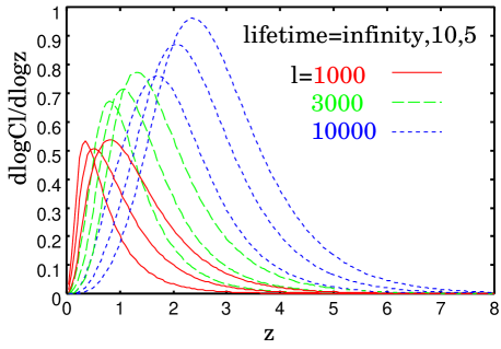
Figure 1: Redshift distribution of $C_{l}$ for a given $l$: $d\ln{C_{l}}/dz$. Solid, dashed and dotted lines correspond to $l=1000,3000,10000$, respectively, and for each $l$, three lines, from the left to right, show model with the dark matter with lifetime of infinity, $10h^{-1}{\rm Gyr}$ and $5h^{-1}{\rm Gyr}$.

It is helpful to see the contribution to $C_{l}$ of cluster with specific mass and redshift. Figure 1 shows the redshift distribution of $C_{l}$ for a given $l$: $d\ln{C_{l}}/dz$. Solid, dashed and dotted lines correspond to $l=1000,3000,10000$, respectively, and for each $l$, three lines, from the left to right, show model with the dark matter with lifetime of infinity, $10h^{-1}{\rm Gyr}$ and $5h^{-1}{\rm Gyr}$. It can be easily understood that clusters at a higher redshift contribute to power of a larger $l$, that is, a smaller scale. Since the angular-diameter distance at a given redshift become shorter with shorter lifetime of the dark matter, the peaks move toward high-redshift side as the lifetime becomes small for each $l$.

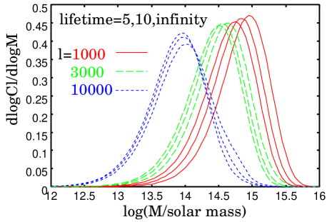
Figure 2: Mass distribution of $C_{l}$ for a given $l$: $d\ln{C_{l}}/d\ln{M}$. Solid, dashed and dotted lines correspond to $l=1000,3000,10000$, respectively, and for each $l$, three lines, from the left to right, show model with the dark matter with lifetime of , $5h^{-1}{\rm Gyr}$, $10h^{-1}{\rm Gyr}$ and infinity. Note that the order of the lifetime is opposite to Figure 1.

Figure 2 shows the redshift distribution of $C_{l}$ for a given $l$: $d\ln{C_{l}}/d\ln{M}$. Types of lines for each $l$ are the same as those in Figure 1 but the order of the lifetime is opposite to that in Figure 1. It can be easily understood that clusters of larger mass contribute to power of a smaller $l$, that is, larger scale. The peaks move toward low-mass side with shorter lifetime because the angular-diameter distance at a given redshift become shorter.

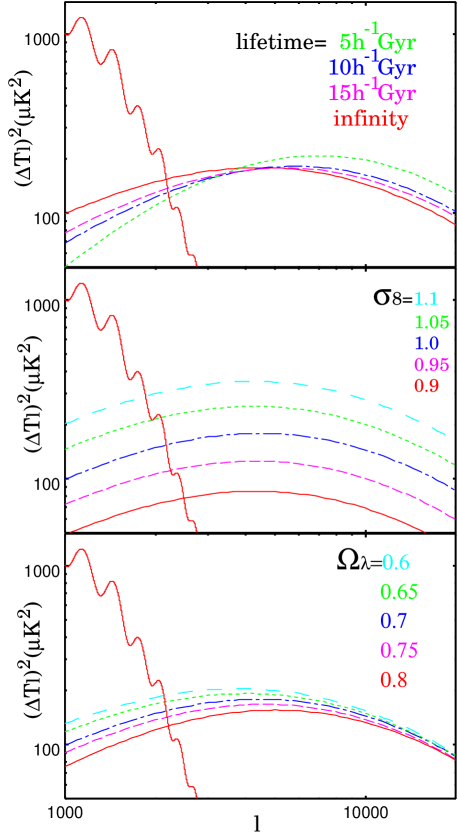
Figure 3: Dependence of the angular power spectrum on the lifetime of the dark matter, $\sigma_{8}$ and $\Omega_{\lambda}$. The fiducial model is the universe with stable dark matter, $\sigma_{8}=1.0,\Omega_{\lambda}=0.7$ and $h=0.7$. The primary spectrum is also shown.

In Figure 3, we show the dependence of the angular power spectrum on several cosmological parameters. Besides the lifetime of dark matter, we choose $\sigma_{8}$ and $\Omega_{\lambda}$ as main parameters. The reasons are (1) it is known that the SZ angular power spectrum is quite sensitive to $\sigma_{8}$, and rather insensitive to other parameters (Komatsu & Seljak, 2002), (2) the SZ angular power spectrum is also sensitive to baryon matter density $\Omega_{\rm b}h^{2}$, where $h$ is the Hubble constant in units of $100{\rm km\,s^{-1}Mpc^{-1}}$, but now it is accurately measured by CMB anisotropy (Spergel et al., 2003), and (3) $\Omega_{\lambda}$ usually degenerates with the lifetime of dark matter (Ichiki et al., 2003; Oguri et al., 2003), thus we should see how we can determine the lifetime of dark matter and $\Omega_{\lambda}$ separately. The fiducial model here is the universe with stable dark matter, $\sigma_{8}=1.0$, $\Omega_{\lambda}=0.7$, $\Omega_{\rm b}h^{2}=0.02$, and $h=0.7$. As can be seen in the top figure, the power at large $l$ increase and that at small $l$ decrease with shorter lifetime. This behavior is mainly because of the milder evolution of the cluster abundance in decaying cold dark matter model. The signal for a given multipole $l$ is from clusters which angular sizes roughly corresponds to $l^{-1}$, so nearby clusters contribute low-$l$ (see Figure 1). Since the decay of dark matter lowers the ratio of low-$z$ to high-$z$ clusters, it tilts the angular power spectrum so that signals at large $l$ increase. On the other hand, the value of $\sigma_{8}$ increases or decreases the normalization of the angular power spectrum and does not change the shape. The effect of changing $\Omega_{\lambda}$ is also nearly scale-independent. From these different dependences, we expect that we can determine these three parameters rather separately.

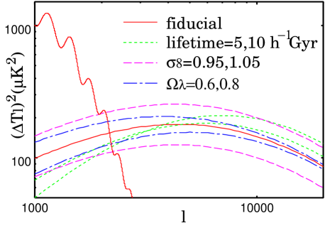
Figure 4: Comparison of the strength of the dependence of the lifetime, $\sigma_{8}$ and $\Omega_{\lambda}$ on the power spectrum. The fiducial model is the same as in Figure 3. The primary spectrum is also shown.

The comparison of the strength of the dependence of each parameter is shown in Figure 4. From this Figure, we find that the difference of signals by changing the lifetime by a factor 2 roughly corresponds to the change of $\sigma_{8}$ by a few percents or $\Omega_{\lambda}$ by a few tens percents.

4.2 Sensitivity of future experiment

In this subsection we investigate how well we can probe the lifetime of dark matter with future SZ surveys. We do not specify the instruments but consider a survey with $100{\rm deg}^{2}$ field of view, beam size of $1^{\prime}$ and sensitivity $2\mu{\rm K}$. These are typical values for near-future experiments such as ACT, AMIBA and BOLOCAM (Komatsu & Seljak, 2002; Zhang et al., 2002; Glenn et al., 2003).

To investigate the sensitivity for cosmological parameters, we use the Fisher information matrix approach (Seljak, 1996; Jungman et al., 1996; Zaldarriaga & Seljak, 1997; Eisenstein et al., 1999). Because this approach is based on the dependence of power spectrum on the cosmological parameters, results would be rather insensitive to the underestimation of halo abundance due to the Press-Schechter mass function. Under the assumption of Gaussian perturbations and Gaussian noise, the Fisher matrix for CMB anisotropies is,

$$F_{ij}=\sum_{l}\frac{\partial C_{l}}{\partial p_{i}}({\rm Cov}_{l})^{-1}\frac{\partial C_{l}}{\partial p_{j}},$$ (24)

where $p_{i}$ is a cosmological parameter and the covariance matrix ${\rm Cov}_{l}$ is,

$${\rm Cov}_{l}=\frac{2}{(2l+1)f_{\rm sky}}\left[C_{l}+\theta_{\rm beam}^{2}\sigma^{2}\exp{\left\{\frac{l(l+1)}{8\ln{2}}\theta_{\rm beam}^{2}\right\}}\right].$$ (25)

Here $f_{\rm sky}$ is a fraction of the surveyed sky, $\theta_{\rm beam}$ is the full width, half-maximum of the beam in radians, and $\sigma$ is sensitivity in $\mu{\rm K}$. We use the values stated at the beginning of this subsection for these parameters. Summation with respect to $l$ is taken from $l=3000$ to $l=20000$, in order for the primary power to be negligible. As discussed in §4.1, we adopt the lifetime $\Gamma^{-1}$, $\sigma_{8}$, and $\Omega_{\lambda}$ as main parameters which we vary. We fix the Hubble constant to $h=0.7$ and the baryon density $\Omega_{\rm b}h^{2}=0.02$. Figure 5 is marginalized 1-$\sigma$ contour for these three parameters for a cosmological model with $\Gamma^{-1}=10h^{-1}{\rm Gyr}$, $\sigma_{8}=1.0$, and $\Omega_{\lambda}=0.7$. As can be seen, the lifetime can be determined by a factor of two or so. On the other hand, $\sigma_{8}$ and $\Omega_{\lambda}$ will be determined within $\pm 0.04$ and $\pm 0.15$, respectively.

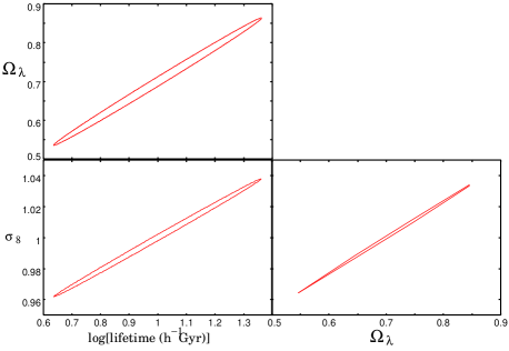
Figure 5: Marginalized 1-$\sigma$ contour for $\Gamma,\sigma_{8}$, and $\Omega_{\lambda}$ for a cosmological model with $\Gamma^{-1}=10h^{-1}{\rm Gyr}$, $\sigma_{8}=1.0$, and $\Omega_{\lambda}=0.7$.

It should be noted that there are some theoretical uncertainties in the SZ power spectrum. Komatsu & Seljak (2002) found that uncertainties due to the mass function, concentration parameter, outer radius of the gas profile and the effect of temperature decrease within $5\%$ of the virial radius are negligible. da Silva et al. (2001b) showed by hydrodynamical simulations that the effect of non-adiabatic physics, such as radiative cooling and preheating, reduces $C_{l}$ by 20-40$\%$ on all angular scales. This seems a significant uncertainty because the effect of finite lifetime is not so large. However, since this uncertainty does not change the shape of the spectrum but just changes the normalization, it is expected that it does not weaken the constraint on the lifetime while it affects the determination of $\sigma_{8}$ and $\Omega_{\lambda}$. Of course, we need more accurate mass functions when we compare the theoretical predictions with real observational data and constrain the lifetime.

5 SUMMARY

In this paper, we studied the effect of finite lifetime of dark matter on SZ power spectrum. We calculated the SZ power spectrum following the method proposed by Komatsu & Seljak (2002) using the Press-Schechter mass function and taking the decay width of dark matter into account. We have found that the finite lifetime of dark matter decreases the power at large scale ($l<4000$) and increases at small scale ($l>4000$). This unique feature will allow us to probe the lifetime of dark matter, rather independently with $\sigma_{8}$ and $\Omega_{\rm m}$ which mainly change the normalization of the angular power spectrum. Then we estimated how well we can constrain the lifetime in the future CMB experiment such as ACT, AMIBA and BOLOCAM. An SZ survey with $100{\rm deg}^{2}$ field of view, beam size of $1^{\prime}$ and sensitivity $2\mu{\rm K}$, which are the representative values of the near-future experiment, will be able to determine the lifetime within factor of two if the lifetime is $10h^{-1}{\rm Gyr}$ even if we marginalized other parameters such as $\sigma_{8}$ and $\Omega_{\rm m}$. Therefore, future SZ surveys will definitely provide an opportunity to reveal the nature of dark matter.

References

- Bardeen et al. (1986) Bardeen, J. M., Bond, J. R., Kaiser, N., & Szalay, A. S. 1986, ApJ, 304, 15
- Battye & Weller (2003) Battye, R. A., & Weller, J. 2003, Phys. Rev. D, 68, 083506
- Benakli et al. (1999) Benakli, K Ellis, J. R. & Nanopoulos, D. V. 1999, Phys. Rev. D, 59, 047301
- Bond et al. (2002) Bond, J. R., et al. 2002, ApJ, submitted (astro-ph/0205386)
- Carlstrom et al. (2002) Carlstrom, J., Holder, G. P., & Reese, E. D. 2002, ARA&A, 40, 643
- Cen (2001) Cen, R. 2001, ApJ, 546, L77
- Chou & Ng (2003) Chou, C-H., & Ng, K-W. 2003, astro-ph/0306437
- Chung et al. (1998) Chung, D. J. H., Kolb, E. W., & Riotto, A. 1998, Phys. Rev. Lett., 81, 4048
- da Silva et al. (2000) da Silva, A. C., Barbosa, D., Liddle, A. R., & Thomas, P. A. 2000, MNRAS, 317, 37
- da Silva et al. (2001a) da Silva, A. C., Barbosa, D., Liddle, A. R., & Thomas, P. A. 2001a, MNRAS, 326, 155
- da Silva et al. (2001b) da Silva, A. C., Kay, S. T., Liddle, A. R., Thomas, P. A., Pearce, F. R., & Barbosa, D. 2001b, MNRAS, 326, 155
- Dawson et al. (2002) Dawson, K. S., Holzapfel, W. L., Carlstrom, J. E., Joy, M., LaRoque, S. J., Miller, A. D., Nagai, D. 2002, ApJ, 581, 86
- Diego et al. (2003) Diego, D. M., Mazzotta, P., & Silk, J. 2003, ApJ, 597, L1
- Dolgov & Zeldovich (1981) Dolgov, A. D. & Zeldovich, Y. B. 1981, Rev. Mod. Phys. 53, 1
- Dubovsky et al. (2000) Dubovsky, S. L., Rubakov, V. A., & Tinyakov, P. G. 2000, Phys. Rev. D, 62, 105011
- Eisenstein et al. (1999) Eisenstein, D. J., Hu, W., & Tegmark, M. 1999, ApJ, 518, 2
- Glenn et al. (2003) Glenn, J., et al., 2003, in Millimeter and Submillimeter Detectors for Astronomy, eds T. G. Phillips, J. P. Zmuidzinas, Proceedings of the SPIE, volume 4855, page 30
- Gomez et al. (2003) Gomez, P., et al., astro-ph/0311263
- Hagiwara & Uehara (2001) Hagiwara, K., Uehara, Y. 2001, Phys. Lett. B, 517, 383
- Hughes & Birkinshaw (1998) Hughes, J. P., & Birkinshaw, M. 1998, ApJ, 501, 1
- Ichiki et al. (2003) Ichiki, K., Garnavich, P. M., Kajino, T., Mathews, G. J., & Yahiro, M. 2003, Phys. Rev. D, 68, 083518
- Jenkins et al. (2001) Jenkins, A., Frenk, C. S., White, S. D. M., Colberg, J. M., Cole, S., Evrard, A. E., Couchman, H. M. P., & Yoshida, N. 2001, MNRAS, 321, 372
- Jungman et al. (1996) Jungman, G., Kamionkowske, M., Kosowsky, A., & Spergel, D. N. 1996, Phys. Rev. Lett., 76, 1007
- Kay et al. (2001) Kay, S. T., Liddle, A. R., & Thomas, P. A. 2001, MNRAS, 325, 835
- Kim & Kim (2002) Kim, H. B. & Kim, J. E. 2002, Phys. Lett. B, 527 18
- Kitayama et al. (2003) Kitayama, T., Komatsu, E., Ota, N., Kuwabara, T., Suto, Y., Yoshikawa, K., Hattori, M., & Matsuo, H. 2003, PASJ, accepted (astro-ph/0311574)
- Kitayama & Suto (1996) Kitayama, T., & Suto, Y. 1996, ApJ, 469, 480
- Komatsu & Kitayama (1999) Komatsu, E., & Kitayama, T. 1999, ApJ, 526, L1
- Komatsu & Seljak (2001) Komatsu, E., & Seljak, U. 2001, MNRAS, 327, 1353
- Komatsu & Seljak (2002) Komatsu, E., & Seljak, U. 2002, MNRAS, 336, 1256
- Kuo et al. (2002) Kuo, C. L., et al. 2002, ApJ, submitted (astro-ph/0212289)
- Kuzmin & Tkachev (1998) Kuzmin, V. A., & Tkachev, I. I. 1998, JETP Lett., 68, 271
- Lacey & Cole (1993) Lacey, C., & Cole, S. 1993, MNRAS, 262, 627
- Lee (2002) Lee, J. 2003, ApJ, 578, L27
- Lee & Yoshida (2003) Lee, J., & Yoshida, N. 2003, ApJ, submitted (astro-ph/0311269)
- Makino & Suto (1993) Makino, N., & Suto, Y. 1993, ApJ, 405, 1
- Mason et al. (2003) Mason, B. S., et al., 2003, ApJ, 591, 540
- Navarro, Frenk, & White (1997) Navarro, J. F., Frenk, C. S., & White, S. D. M. 1997, ApJ, 490, 493
- Oguri et al. (2003) Oguri, M., Takahashi, K., Ohno, H., & Kotake, K. 2003, ApJ, 597, 645
- Oh et al. (2003) Oh, S. P., Cooray, A., & Kamionkowski, M. 2003, MNRAS, 342, L20
- Ostriker & Steinhardt (2003) Ostriker, J. P., & Steinhardt, P. 2003, Science, 300, 1909
- Press & Schechter (1974) Press, W. H., & Schechter, P. 1974, ApJ, 187, 425
- Randall & Sundrum (1999a) Randall, L., & Sundrum, R. 1999a, Phys. Rev. Lett. 83, 3370
- Randall & Sundrum (1999b) Randall, L., & Sundrum, R. 1999b, Phys. Rev. Lett. 83, 4690
- Seljak (1996) Seljak, U. 1996, ApJ, 482, 6
- Seljak (2000) Seljak, U. 2000, MNRAS, 318, 203
- Seljak et al. (2001) Seljak, U., Burwell, J., & Pen, U. 2001, Phys. Rev. D, 63, 619
- Spergel et al. (2003) Spergel, D. N., et al. 2003, ApJS, 148, 175
- Sunyaev & Zel’dovich (1972) Sunyaev, R. A., & Zel’dovich, Ya. B. 1972, Comments Astrophys. Space Phys. 4, 173
- Yoshikawa & Suto (1999) Yoshikawa, K., & Suto, Y. 1999, ApJ, 513, 549
- Zaldarriaga & Seljak (1997) Zaldarriaga, M., & Seljak, U. 1997, Phys. Rev. D, 55, 1830
- Zaroubi et al. (1998) Zaroubi, S., Squires, G., Hoffman, Y., & Silk, J. 1998, ApJ, 500, L87
- Zhang & Pen (2001) Zhang, P. J., & Pen, U. L. 2001, ApJ, 549, 18
- Zhang et al. (2002) Zhang, P. J., Pen, U. L., & Wang, B. 2002, ApJ, 577, 555
- Zhang et al. (2003) Zhang, P. J., Pen, U. L., & Trac, H. 2003, MNRAS, accepted (astro-ph/0304534)
- Zhang (2003) Zhang, P. J. 2003, MNRAS, submitted (astro-ph/0308354)
- Ziaeepour (2001) Ziaeepour, H. 2001, Astropart. Phys. 16, 101