Misleading results from low-resolution spectroscopy: from galaxy interstellar medium chemistry to cosmic star formation density

Low resolution spectroscopy (R=150) from the Canada-France-Redshift Survey (CFRS) had revealed intriguing properties for low redshift galaxies (z$\leq$ 0.3): nearly half of their spectra show prominent $H\alpha$ emission line, but no $H\beta$ emission line and barely detected [O ii] $\lambda$3727, and [O iii] $\lambda$5007 lines. We call these objects “CFRS H$\alpha$-single” galaxies and have re-observed a subsample of them at higher spectral resolution, associated with a subsample of more normal emission line galaxies. Good S/N spectroscopy at the VLT and the CFHT, with moderate spectral resolution (R$>$600), have allowed us to perform a full diagnostic of their interstellar medium chemistry. “CFRS H$\alpha$-single” galaxies and most of the star forming spirals are with high extinctions ($A_{V}>2$), high stellar masses and over-solar oxygen abundances.
From the present study, we believe hazardous to derive the detailed properties of galaxies (gas chemical abundances, interstellar extinction, stellar population, star formation rates and history) using spectra with resolutions below 600. One major drawback is indeed the estimated extinction which requires a proper analysis of the underlying Balmer absorption lines. We find that, with low resolution spectroscopy, star formation rates (SFRs) can be either underestimated or overestimated by factors reaching 10 (average 3.1), even if one accounts for ad hoc extinction corrections. These effects are prominent for a large fraction of evolved massive galaxies especially those experiencing successive bursts (A and F stars dominating their absorption spectra). Further estimates of the cosmic star formation density at all redshifts mandatorily requires moderate resolution spectroscopy to avoid severe and uncontrolled biases.

1 Introduction

Star formation history is a fundamental quantity to study the populations and evolution of galaxies. Hot, massive, short-lived OB stars emit ultraviolet (UV) photons which ionize the surrounding gas to form an H II region, where the recombinations produce spectral emission lines. Among the Balmer lines, H$\alpha$ is the most directly proportional to the ionizing UV stellar spectra at $\lambda<$912Å  (Osterbrock 1989), and the weaker Balmer lines are much more affected by stellar absorption and reddening. The other commonly observed metallic optical lines such as [N ii] $\lambda\lambda$6548, 6583, [S ii] $\lambda\lambda$6716, 6731, [O ii] $\lambda$3727, and [O iii] $\lambda\lambda$4958, 5007 depend strongly on the metal fraction present in the gas. Their ionizing potential is higher than the Balmer lines and thus depends on the hardness of the ionizing stellar spectra. These metal lines only represent the indirect tracers of recent star formation, and they characterize the gas chemistry which is linked to the star formation history in individual galaxies. Hence, H$\alpha$ luminosity density is one strong tool to estimate the cosmic star formation density (CSFD).

The optical H$\alpha$ line has been used to estimate the star formation (SF) density in the nearby universe. Tresse & Maddox (1998, hereafter TM98) have calculated the H$\alpha$ luminosity density at z$\sim$ 0.2 on the basis of $z<0.3$ CFRS galaxies and have obtained 10^39.44±0.04 ergs s^-1 Mpc^-1. More recent works (Pascual et al. 2001; Fujita et al. 2003), based on deep imaging narrow band data, provided respectively 1.6 and 1.9 times higher than TM98 estimated value. Fujita et al. (2003) argued that their estimates correspond to a redshift (0.24) slightly higher than that sampled by TM98, and also that their data revealed a steeper slope of the faint end of the $H\alpha$ luminosity function.

The above works were based on narrow band filter data and spectroscopy of very low resolving powers (R from 65 to 150) and they made crude assumptions about the extinction coefficient to be applied on the H$\alpha$ luminosity. Indeed, at low resolving power, the underlying Balmer absorption, related to intermediate age stellar populations, can severely affect the H$\alpha$/H$\beta$ ratio used to estimate the extinction coefficient.

In this paper, our aim is to address two questions: (1) could we estimate the global properties (gas chemical abundances, extinction and SFRs) of individual galaxies on the basis of low resolution spectroscopy ? (2) How solid are SF density estimates based on low resolution spectroscopy or narrow band filters imagery? To tackle these issues we have gathered a small, but representative sample of low-z galaxies and have systematically compared their properties derived from different spectral resolution observations, the very low and the moderate ones. Low resolution spectroscopy (about 40Å ) was provided by the CFRS spectra, and moderate resolution spectra have been obtained by using the European Southern Observatory (ESO) Very Large Telescope (VLT) and the Canada-France-Hawaii Telescope (CFHT): VLT/FORS and CFHT/MOS (5Å  or 12Å  for VLT, 12Å  for CFHT)

The paper is organized as follows. In Sect.2, we describe the sample selection. The observations, data reduction and flux measurements are described in Sect.3. Extinction properties are discussed in Sect.4, allowing to present diagnostic diagrams and the estimated gas abundances in Sect. 5. The derived SFRs of these galaxies were given in Sect. 6, which includes a discussion on the requirements needed for proper estimates. For reasons of consistency with the former analyses, the adopted cosmological constants are $H_{0}$=50 km s^-1 Mpc^-1 and $q_{0}=0.5$ throughout this paper.

2 CFRS low redshift galaxies: the sample selection

CFRS has produced a unique sample of 591 field galaxies with $I_{AB}<22.5$ in the range 0$<$ $z$ $<$1.3 with a median $\langle z\rangle\sim 0.56$ (Lilly et al. 1995a , Le Fèvre et al. CFRS2 (1995), Lilly et al. 1995b ; Hammer et al. CFRSIV (1995); Crampton et al. CFRS5 (1995)), which is a good sample to study stellar formation history, stellar population and evolution of galaxies.

There are 138 CFRS galaxies with z $\leq$ 0.3 showing both H$\alpha$ and H$\beta$ lines in the rest-frame optical wavelength range. 21 of these galaxies exhibit both H$\alpha$ and H$\beta$ in absorption, and 117 exhibit H$\alpha$ emission lines (see Fig. 1). Among the 117 low-$z$ H$\alpha$ emission galaxies, 57 ($\sim$49%) of them exhibit non-positive equivalent width of H$\beta$, EW(H$\beta$)$\leq 0$, (zero in 43 and negative in 14 galaxies), and generally exhibit no [O iii] $\lambda 5007$, [O ii] $\lambda 3727$ emission lines (Hammer et al. hammer97 (1997); Hammer and Flores HF01 (2001); Tresse et al. 1996). We call these galaxies “CFRS H$\alpha$-single” galaxies. 53 of the H$\alpha$-emission line galaxies show EW(H$\beta)>0$, which are called as “CFRS normal emission line” galaxies in this study. The other 7 are without available information about H$\beta$ because of the weak quality of their spectra near to 4861Å  wavelength (Tresse et al. 1996; Hammer et al. 1997).

Why almost half of the CFRS low-$z$ sample galaxies exhibit “H$\alpha$-single” spectra ? Could it be due to large extinctions? Is it related to the low spectral resolution in the CFRS ? Or could it be due to the “fact” that they are “peculiar” objects? What is the difference or relation between the “H$\alpha$-single” galaxies and other “normal emission line” galaxies?

Seven “CFRS H$\alpha$-single” galaxies are selected to understand their detailed properties (the filled circles on Fig. 1). Another nine “CFRS normal emission line” galaxies (showing both H$\alpha$ and H$\beta$ in emission) are associated to be selected for comparison mainly (the squares on Fig. 1). They can be the representatives of the two group galaxies mentioned above as demonstrated in Fig. 1 though all of them were observed during observational runs targetting different goals (higher redshift galaxies) by completing MOS or FORS masks.

The properties of the 16 sample galaxies are studied by using moderately high resolution and high S/N spectra from the VLT and the CFHT. Their images were obtained by the Hubble Space Telescope (HST) WFPC2 with filter F814W in 1994 and the CFHT/FOCAM in 1991. The basic data for these galaxies are given in Table 1. The columns are CFRS name, redshift, $I_{AB}$ magnitude, absolute B magnitude, $K_{AB}$ and absolute K magnitudes (“9999” was marked for the absent values), and the telescopes used for spectral and imaging observations. All the magnitudes are in the AB systems.

Table 1: Basic data of the sample galaxies, the top seven are the “CFRS H$\alpha$-single” galaxies, the bottom nine are the “CFRS normal emission line” galaxies. “SPE” means “spectroscopy” and “IMA” means “imagery”

Objects	$z$	$I_{AB}$	$M_{B}$	$K_{AB}$	$M_{K}$	SPE	IMA
03.0364	0.2511	19.05	$-$20.79	17.89	$-$22.63	CFHT	HST
03.0365	0.2183	19.19	$-$20.09	17.91	$-$22.20	CFHT	HST
03.0578	0.2192	20.79	$-$19.16	20.07	$-$20.04	VLT600	HST
03.0641	0.2613	20.03	$-$19.62	9999	9999	VLT600	CFHT
03.0711	0.2615	21.04	$-$19.03	19.76	$-$20.92	VLT600	HST
03.1014	0.1961	18.42	$-$20.87	17.27	$-$23.10	CFHT	HST
22.0717	0.2791	19.60	$-$20.24	17.92	$-$23.04	VLT300	CFHT
03.0003	0.2187	22.49	$-$16.60	21.81	$-$18.18	CFHT	CFHT
03.0149	0.2510	20.74	$-$19.42	19.70	$-$20.82	VLT600	HST
03.0160	0.2184	21.83	$-$17.71	9999	9999	CFHT	CFHT
03.1299	0.1752	18.59	$-$20.47	9999	9999	CFHT	HST
03.1311	0.1755	19.56	$-$19.40	18.05	$-$22.23	CFHT	HST
14.1103	0.2080	22.33	$-$17.69	9999	9999	CFHT	CFHT
14.1117	0.1919	20.79	$-$18.98	9999	9999	CFHT	CFHT
22.0474	0.2801	21.74	$-$18.66	21.12	$-$19.55	VLT300	CFHT
22.1084	0.2930	20.29	$-$20.22	19.22	$-$21.70	CFHT	CFHT

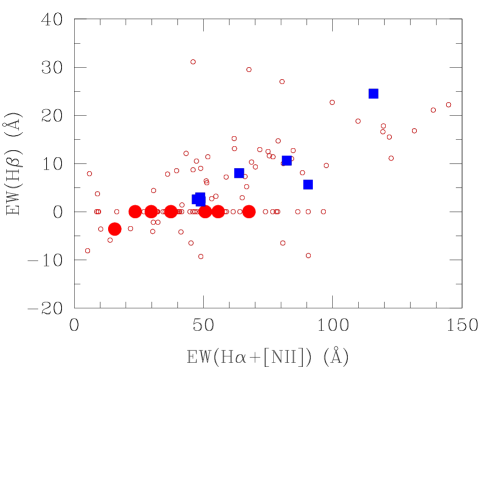
Figure 1: EW(H$\beta$) against EW(H$\alpha$+[N ii]) for the 117 H$\alpha$ emission CFRS galaxies ($z$$\leq$0.3) (open circles) at rest-frame. Five galaxies are outside the diagram, having higher EW(H$\alpha$+[N ii]) than 150 Å, including two sample galaxies in this study, CFRS22.0474 with (370, 42) and CFRS14.1103 with (2940, 192). The large filled circles represent the “CFRS H$\alpha$-single” galaxies. The filled squares represent the “CFRS normal emission line” galaxies.

3 Observations, data reduction and flux measurements

Spectrophotometric observations for four sample galaxies were obtained during one night (for 3^h field) with the ESO 8m VLT/FORS2 instrument with the R600 and I600 grisms (R=5Å) and covering the wavelength range from 5500 to 9200Å. The slit width was 1.2^′′, and the slit length 10^′′. The objects CFRS22.0474 and CFRS22.0717 were observed in another night (for 22^h field) using the VLT/FORS2 instruments with the R300 grism (R=12Å) and covering the wavelength range from 5800 to 9500Å. The slit width was 1.0″, and the slit length 10^′′. CFHT data were obtained in different runs from 1996 to 1999, using the standard MOS setup with the R300 grism and a 1.5^′′ slit. These ensure the coverage from H$\beta$ to [S ii] lines in the rest-frame spectrum.

The spectra were extracted and wavelength-calibrated using IRAF packages. Flux calibration was done using 15 minute exposures of different photometric standard stars. To ensure the reliability of the data, all spectrum extractions, as well as the lines measurements, were performed by using the SPLOT program.

The rest-frame spectra of the 16 sample galaxies are given in Fig. 2(a-o) and Fig. 3(a),(b). The continua have been convolved except at the locations of the emission lines (e.g. H$\beta$; [O iii] $\lambda\lambda$4958, 5007; [N ii] $\lambda\lambda$6548, 6583; H$\alpha$ and [S ii] $\lambda\lambda$6716, 6731) using the procedure developed by our group (Hammer et al. hammer01 (2001); Gruel Gruel02 (2002); Gruel et al. Gruel03 (2003)). For the VLT600 spectra, the adopted convolution factors are 7 pixels and then 15 pixels; for the VLT300 and CFHT spectra, the convolution factors are 7 and 7 pixels (Hammer et al. hammer01 (2001); Gruel et al. Gruel03 (2003)). Pairs of vertical dashed lines delimit the regions where strong sky emission lines (e.g. [O i] 5577, 6300, 6364Å  and OH 6834, 6871, 7716, 7751, 7794, 7851, 7914, 7993, 8289, 8298, 8344, 8505Å) and absorption lines (O₂ 6877, 7606 and 7640Å) are located. Fig. 2(a$\arcmin$-o$\arcmin$) and Fig. 3(c),(d) give the corresponding CFRS low-resolution spectra of the galaxies. The comparison between the moderate-resolution spectra and the CFRS spectra show that the emission lines are strongly hidden or diluted in the low resolution observations. And the higher resolution make it possible to separate the [N ii] $\lambda\lambda$6548, 6583 emission lines from the H$\alpha$ emission.

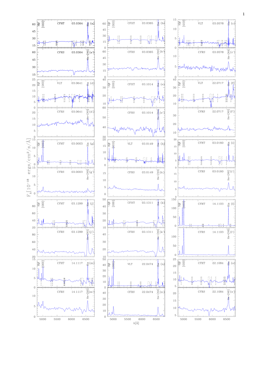
Figure 2: (a)-(o) Rest-frame spectra of 15 sample galaxies from the moderate-resolution observations ; (a$\arcmin$)-(o$\arcmin$) the corresponding low-resolution CFRS spectra of the galaxies. (a)-(f) and (a$\arcmin$)-(f$\arcmin$) are the spectra of the six “CFRS H$\alpha$-single” galaxies, others are the spectra of the nine “CFRS normal emission line” galaxies. The spectrum of another “CFRS H$\alpha$-single” galaxy, CFRS03.0711, will be given in Fig. 3.

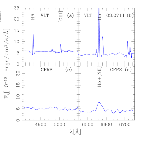
Figure 3: (a), (b) Rest-frame spectra of CFRS03.0711 from the VLT observation around H$\beta$ and H$\alpha$ wavelength positions; (c), (d) The corresponding low-resolution CFRS spectra.

The fluxes of emission lines have been measured using the SPLOT package. The stellar absorption under the Balmer lines are estimated from the synthesized stellar spectra obtained using the stellar spectra of Jacoby et al. (Jacoby84 (1984)). The corresponding error budget has been deduced using three independent methods: the first one is estimated by trying several combinations of the stellar templates for the stellar absorption; the second one is from measurement, which is estimated according to the independent measurements performed by Y.C. Liang, H. Flores and F. Hammer; the third one is Poisson noises from both sky and objects. The flux measurements of the emission lines from the VLT and the CFHT spectra and their errors are given in Table 2. The fluxes of [O ii]$\leavevmode\nobreak\ \lambda 3727$ are estimated from the original CFRS spectra with large error bars due to the absence of this line in the rest-frame wavelength ranges of the moderate resolution spectra.

Table 2: Measured emission fluxes (F_λ) of the sample galaxies in units of 10^-17 ergs cm^-2 s^-1, “9997” means the line is blended with strong sky line, “9998” means there are no the corresponding lines detected around the line positions, and “9999” means the lines are shifted outside the observed wavelength ranges. “Ap” is the aperture correction factor between the CFRS and the present moderate-resolution observations due to the different slit widths

CFRS	H$\beta$ 4861	[O iii]4958	[O iii]5007	H$\alpha$6563	[N ii]6548	[N ii]6583	[S ii]6716	[S ii]6731	[S ii]1+2	[O ii]3727	Ap
03.0364	7.18$\pm$0.57	0.81$\pm$0.05	2.44$\pm$0.14	62.30$\pm$0.62	6.89$\pm$0.41	22.3$\pm$1.11	—	—	10.90$\pm$1.50	9999	1.0
03.0365	13.49$\pm$0.54	$<$0.54	$<$1.61	88.75$\pm$8.34	14.25$\pm$1.43	33.14$\pm$2.45	12.55$\pm$1.04	9.32$\pm$0.77	21.87$\pm$1.81	14.0$\pm$14.0	1.0
03.0578	1.23$\pm$0.20	0.61$\pm$0.09	1.77$\pm$0.26	8.76$\pm$0.43	1.06$\pm$0.34	1.80$\pm$0.66	1.80$\pm$0.31	2.07$\pm$0.29	3.87$\pm$0.60	5.3$\pm$1.0	1.8
03.0641	2.21$\pm$0.24	0.31$\pm$0.06	0.92$\pm$0.17	10.25$\pm$0.92	1.18$\pm$0.14	3.53$\pm$0.43	$<$1.38	$<$1.65	$<$3.03	3.0$\pm$1.0	1.3
03.0711	4.49$\pm$0.18	0.65$\pm$0.07	1.95$\pm$0.20	13.58$\pm$0.58	1.04$\pm$0.12	5.78$\pm$0.68	3.56$\pm$0.37	1.96$\pm$0.37	5.52$\pm$0.74	2.5$\pm$2.0	1.0
03.1014	5.90$\pm$0.71	9998	1.32$\pm$0.26	43.28$\pm$4.51	4.24$\pm$0.85	13.00$\pm$1.71	9.26$\pm$0.99	5.12$\pm$2.78	14.38$\pm$3.77	16.0$\pm$7.0	2.2
22.0717	3.54$\pm$0.44	9998	$<$0.75	29.71$\pm$2.67	3.67$\pm$0.40	14.07$\pm$1.55	—	—	9997	1.3$\pm$1.3	1.0
03.0003	3.97$\pm$0.80	5.41$\pm$0.54	16.16$\pm$0.86	13.89$\pm$0.62	—	$<$3.06	2.80$\pm$0.20	1.95$\pm$0.14	4.75$\pm$0.50	2.1$\pm$2.1	0.6
03.0149	4.76$\pm$0.28	1.87$\pm$0.07	5.43$\pm$0.22	17.18$\pm$0.71	1.35$\pm$0.17	3.49$\pm$0.43	3.95$\pm$0.72	2.61$\pm$0.39	6.56$\pm$1.11	7.1$\pm$7.1	1.0
03.0160	4.25$\pm$0.51	1.57$\pm$0.157	4.72$\pm$0.47	12.40$\pm$0.37	—	6.17$\pm$0.66	—	—	7.04$\pm$0.68	9999	1.0
03.1299	16.4$\pm$1.48	5.06$\pm$0.46	15.2$\pm$1.37	144.0$\pm$4.32	13.2$\pm$1.32	39.6$\pm$3.96	—	—	40.0$\pm$4.80	9999	1.0
03.1311	6.97$\pm$0.49	2.53$\pm$0.20	7.59$\pm$0.61	58.4$\pm$2.34	4.40$\pm$0.18	13.4$\pm$0.54	16.5$\pm$1.65	10.5$\pm$1.05	27.0$\pm$2.7	9999	1.0
14.1103	60.56$\pm$0.61	130.9$\pm$0.52	392.7$\pm$1.57	133.9$\pm$0.54	9998	9998	—	—	9998	$<$3.45	1.0
14.1117	5.54$\pm$0.44	3.34$\pm$0.20	10.03$\pm$0.60	15.9$\pm$0.48	—	2.70$\pm$0.54	—	—	4.08$\pm$0.28	9999	1.0
22.0474	13.04$\pm$0.46	14.05$\pm$0.30	43.70$\pm$1.20	51.97$\pm$2.49	4.20$\pm$0.40	11.97$\pm$2.0	6.90$\pm$0.68	5.80$\pm$0.58	12.70$\pm$1.26	17.0$\pm$2.3	1.0
22.1084	5.23$\pm$0.52	0.94$\pm$0.12	2.82$\pm$0.37	26.9$\pm$2.15	1.70$\pm$0.23	5.11$\pm$0.71	—	—	5.82$\pm$0.64	9999	1.0

Notes: Ap=$({{\rm CFRS}\over{\rm VLT}})_{\rm Aper}$. [S ii]₁₊₂=[S ii]${6716}$+[S ii]${6731}$.

4 Balmer decrement and extinction

The major factor that affects measurements of the true emission fluxes is interstellar extinction. If galaxies are observed at high galactic latitudes, the extinction due to our own Galaxy is negligible ($\sim$0.05 mag), hence most extinction is intrinsic to the observed galaxy. Extinction arising along the line of sight to a target galaxy makes the observed ratio of the flux of two emission lines differ from their ratio as emitted in the galaxy. The extinction coefficient, $c$, can be derived using the Balmer lines H$\alpha$ and H$\beta$:

$$\frac{I(H\alpha)}{I(H\beta)}=\frac{I_{0}(H\alpha)}{I_{0}(H\beta)}10^{-c[f(H\alpha)-f(H\beta)]},$$ (1)

where $I(H\alpha)$ and $I(H\beta)$ are the measured integrated line fluxes, and $I_{0}(H\alpha)/I_{0}(H\beta)$ is the ratio of the fluxes as emitted in the interstellar dust. Assuming case B recombination, with a density of 100 cm^-3 and a temperature of 10⁴ K, the predicted ratio of $I_{0}(H\alpha)$ to $I_{0}(H\beta)$ is 2.86 (Osterbrock 1989).

Using the average interstellar extinction law given by Osterbrock (1989), $f(H\alpha)-f(H\beta)$=$-0.37$, $c$ can be readily determined from Eq.(1). Any corrected emission-line flux, $I_{0}(\lambda)$, can then be estimated by correcting the extinction obtained from Eq.(1) and the following average extinction law taken from Osterbrock (1989). The extinction parameter $A_{V}$ ($V$ for visual) has been calculated following the suggestion of Seaton (Seaton79 (1979)): $A_{V}=E(B-V)R=\frac{cR}{1.47}$ (mag). $R$ which is 3.2, is the ratio of total to selective extinction at $V$. The derived extinction values of the sample galaxies, $A_{V}$, are given in Col. 2 in Table 3. Fig. 4 shows the distributions of galaxy numbers vs. extinction ($A_{V}$) for the “CFRS H$\alpha$-single”, “CFRS normal emission line” galaxies and the combination of these two with a 0.5 bin in $A_{V}$. “CFRS H$\alpha$-single” galaxies mostly display high extinction coefficients (median $A_{V}$=2.2), conversely to “CFRS normal emission line” galaxies (median $A_{V}$=0.6). However, taking all the 16 galaxies together leads to an average extinction coefficient of about $A_{V}$=1.25, which is equivalent to the assumption of Fujita et al. (2003, $A_{H\alpha}$=1.0). No very high extinctions ($A_{V}>$ 3.3) are found in the sample galaxies.

Figure 4: Distribution of the extinction $A_{V}$ in sample galaxies with a binning interval of 0.5: (a) the seven “CFRS H$\alpha$-single” galaxies; (b) the nine “CFRS normal emission line” galaxies; (c) the total 16 sample galaxies.

4.1 Photometry and dust correction

Using the HST and the CFHT images of the sample galaxies, we used the GIM2D software package to calculate the inclination $i$ (the disk axis to the line of sight) and the luminosities ratio of the bulge over the total (B/T) of these galaxies. Table 3 gives the corresponding values. All “CFRS H$\alpha$-single” galaxies show disk properties with B/T ratios lower than 0.5. The B/T values are consistent with the study of Kent (Kent85 (1985)), which showed that the B/T ratio is mainly between 0.4 to 0.0 for Sab–Sc⁺ galaxies (see their Fig. 6) (also see Lilly et al. lilly98 (1998)). Three “CFRS normal emission line” galaxies (CFRS03.0003, 14.1103 and 22.0474) are very compact and the analysis of their CFHT images hardly recover their morphological parameters (which results in large error bars).

Generally, the internal extinction of galaxies increases with the inclination of the disk because the path length through the disk increases roughly as 1 /cos$\,i$ (Giovanelli et al. Gio95 (1995)). Fig. 6 provides a good illustration of this effect, since for galaxies with inclination lower than 45^∘, the median $A_{V}$ is 0.6 which could be compared to 2.2 in the edge-on galaxies.

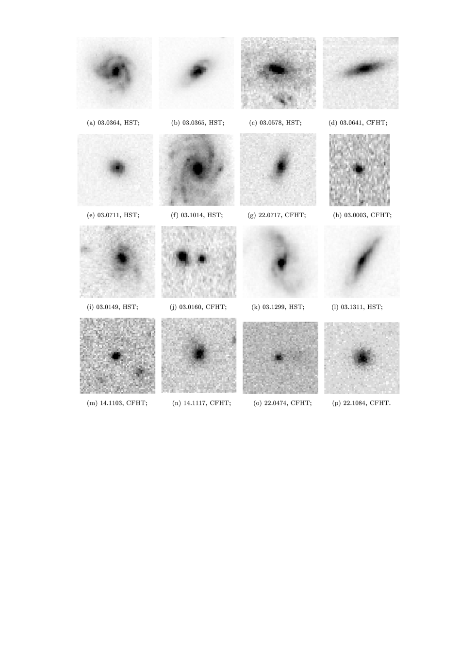
Figure 5: HST/F814W or CFHT images of the sample galaxies. (a)-(g) are the images of the seven “CFRS H$\alpha$-single” galaxies; the rest nine are “CFRS normal emission line” galaxies. Images are 5^′′$\times$5^′′ size, only 03.0003 is 4^′′ in the horizontal size since it is near to the edge of the image of the field.

Table 3: The photometric properties of the sample galaxies

CFRS	$A_{V}$	B/T	inclination $i$
			(degree)
03.0364	2.84$\pm{0.21}$	0.025${}_{-0.002}^{+0.002}$	11${}_{-1}^{+8}$
03.0365	2.13$\pm{0.26}$	0.010${}_{-0.010}^{+0.024}$	59${}_{-1}^{+1}$
03.0578	2.33$\pm{0.44}$	0.214${}_{-0.054}^{+0.047}$	55${}_{-3}^{+4}$
03.0641	1.22$\pm{0.36}$	0.007${}_{-0.007}^{+0.037}$	84${}_{-1}^{+1}$
03.0711	0.14$\pm{0.14}$	0.003${}_{-0.003}^{+0.013}$	32${}_{-3}^{+4}$
03.1014	2.41$\pm{0.41}$	0.021${}_{-0.003}^{+0.157}$	53${}_{-1}^{+4}$
22.0717	2.75$\pm{0.39}$	0.095${}_{-0.095}^{+0.089}$	72${}_{-2}^{+2}$
03.0003	0.52$\pm{0.27}$	0.868${}_{-0.434}^{+0.132}$	17${}_{-17}^{+33}$
03.0149	0.59$\pm{0.18}$	0.333${}_{-0.074}^{+0.150}$	51${}_{-3}^{+4}$
03.0160	0.05${}_{-0.05}^{+0.30}$	0.036${}_{-0.036}^{+0.224}$	23${}_{-23}^{+54}$
03.1299	2.87$\pm{0.24}$	0.097${}_{-0.007}^{+0.071}$	59${}_{-1}^{+2}$
03.1311	2.75$\pm{0.21}$	0.038${}_{-0.013}^{+0.015}$	75${}_{-1}^{+1}$
14.1103	0.00${}_{-0.00}^{+0.02}$	0.817${}_{-0.817}^{+0.183}$	39${}_{-13}^{+19}$
14.1117	0.01${}_{-0.01}^{+0.22}$	0.147${}_{-0.147}^{+0.164}$	47${}_{-13}^{+7}$
22.0474	0.85$\pm{0.13}$	0.898${}_{-0.030}^{+0.020}$	27${}_{-3}^{+4}$
22.1084	1.49$\pm{0.32}$	0.000${}_{-0.000}^{+0.054}$	2${}_{-2}^{+8}$

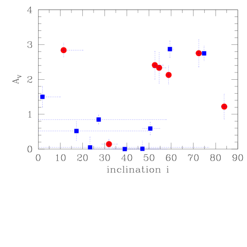
Figure 6: The relations between extinction $A_{V}$ and inclination $i$ in the sample galaxies. Symbols as in Fig. 1.

5 Diagnostic diagrams and gas abundances

5.1 Diagnostic diagrams

Several emission line ratios have been used for a proper diagnostic for the galaxies. Fig. 7(a) and (b) give the diagnostic diagrams of log([O iii] $\lambda{5007}$/H$\alpha$) vs. log([N ii] $\lambda{6583}$/H$\alpha$) and log([O iii] $\lambda{5007}$/H$\alpha$) vs. log([S ii] $\lambda{6716}+\lambda{6731}$/H$\alpha$), respectively.

The [O iii]/H$\beta$ ratio is mainly an indicator of the mean level of ionization and temperature, while the [S ii]/H$\alpha$ ratio is an indicator of the relative importance of a large partially ionized zone produced by high-energy photoionization. The [N ii]/H$\alpha$ ratio also gives a good separation between H II region nuclei and Active Galactic Nuclei (AGN) though its significance is not so immediately obvious. The ratios have been chosen to minimize the effects of dust extinction. (Veilleux & Osterbrock VO87 (1987); Osterbrock Oster89 (1989))

The dashed and dotted lines in the two diagrams are the separating lines between H II region nuclei and AGNs taken from Osterbrock (Oster89 (1989), their Fig. 12.1 and 12.3). The H II region-like objects can be H II regions in external galaxies, starbursts, or H II region galaxies, objects known to be photoionized by OB stars. Seyfert 2 galaxies have relatively high ionization with [O iii] $\lambda{5007}$/H$\beta$$\geq$3. Most starburst and H II region galaxies have lower ionization. Many low-ionization galaxies have stronger [S ii] $\lambda$$\lambda$6716, 6731 and [N ii] $\lambda$6583 than H II regions or starburst galaxies. These objects have been named “Low-Ionization Nuclear Emission-line Regions” (LINERs).

From Fig. 7(a), it seems that all of the sample galaxies are H II-region galaxies except for the possible “LINER” property of CFRS03.0160 due to the strong [N ii] emission. Fig. 7(b) confirms again that most of the studied galaxies lie in the H II-region locus though few of them are in the active region locus (LINER or Seyfert), including CFRS03.0160. Shock-wave ionization may produce stronger [S ii] $\lambda\lambda{6716,6731}$ emissions relative to H$\alpha$ than in typical H II regions. For some of the best quality spectra, we have been able to estimate the intensity ratio of the two [S ii] emission line, ([S ii]$\lambda{6716}$)/([S ii]$\lambda{6731}$) which can be used to estimate the electron density, N_e (Osterbrock Oster89 (1989), p134, their Fig. 5.3). It results the values which are generally close to what is expected from H II region galaxies (may also see van Zee et al. Zee98 (1998)).

From the combination of Fig. 7(a) and (b), we find that it seems that only one object (CFRS03.0160) out of 16 could be a LINER. Moderate resolution spectroscopy is required to establish these two diagnostic diagrams, and is unique for solid estimates of the nature of emission line objects. As also noticed by Tresse et al. (1996), a large fraction of their assumed Seyfert 2 galaxies would be better classified as LINERs if the underlying absorption under the $H\beta$ line was properly accounted for.

In both Fig. 7(a) and (b), the “CFRS H$\alpha$-single” galaxies and the “CFRS normal emission line” galaxies lie in well distinct areas, with the noticeable exception of CFRS03.0578. We believe this is related to different gas metal abundance histories in these two classes of galaxies as it is studied in the following sections.

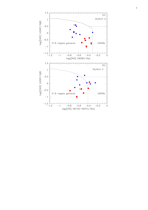
Figure 7: (a) [O iii]/H$\beta$ vs. [N ii]/H$\alpha$ diagnostic diagram for the sample galaxies; (b) [O iii]/H$\beta$ vs. [S ii]/H$\alpha$ diagnostic diagram for the sample galaxies. Symbols as in Fig. 1.

Table 4: The derived emission line ratios and oxygen, nitrogen abundances of the sample galaxies. The first seven are the “CFRS H$\alpha$-single” galaxies, and the rest nine are the “CFRS normal emission line” galaxies

CFRS	log${[O\textsc{iii]}}\over{{\rm H}\beta}$	log${[N\textsc{ii]}}\over{{\rm H}\alpha}$	log${[S\textsc{ii]}}\over{{\rm H}\alpha}$	log${[O\textsc{ii]}}\over{{\rm H}\beta}$	${{[S\textsc{ii]}}_{1}}\over{{[S\textsc{ii]}}_{2}}$	Ne	log(R23)	12+log(O/H)	t${}_{{[N\textsc{ii]}}}$ (K)	log(N/O)
						(cm-3)
03.0364	$-$0.55$\pm$0.04	$-$0.45$\pm$0.02	$-$0.77$\pm$0.06	0.30$\pm$0.30	—	—	0.38$\pm$0.26	9.09$\pm$0.17	7082$\pm$1095	$-$0.90$\pm$0.01
03.0365	$<$$-$0.98	$-$0.43$\pm$0.05	$-$0.63$\pm$0.05	0.29$\pm$0.47	1.35$\pm$0.22	$\sim$102	$<$0.32	$>$9.13	$<$6861	$\sim$$-$0.86
03.0578	0.09$\pm$0.08	$-$0.69$\pm$0.16	$-$0.37$\pm$0.07	0.68$\pm$0.22	0.87$\pm$0.27	$\sim$9$\times$102	0.81$\pm$0.13	8.61$\pm$0.23	10074$\pm$1343	$-$1.12$\pm$0.18
03.0641	$-$0.42$\pm$0.08	$-$0.47$\pm$0.04	$<$$-$0.54	0.17$\pm$0.24	0.84$\pm$0.53	$\sim$103	0.30$\pm$0.16	9.13$\pm$0.09	6798$\pm$571	$-$0.82$\pm$0.19
03.0711	$-$0.37$\pm$0.04	$-$0.37$\pm$ 0.05	$-$0.39$\pm$0.06	$-$0.24$\pm$0.37	1.81$\pm$0.54	$<$101	0.06$\pm$0.20	9.24$\pm$0.07	6173$\pm$375	$-$0.47$\pm$0.38
03.1014	$-$0.7$\pm$0.10	$-$0.53$\pm$0.07	$-$0.49$\pm$0.09	0.40$\pm$0.48	1.81$\pm$0.70	$<$101	0.44$\pm$0.23	9.05$\pm$0.17	7384$\pm$1135	$-$1.02$\pm$0.58
22.0717	$<$$-$0.75	$-$0.33$\pm$0.06	0.07$\pm$0.05	$-$0.08$\pm$0.49	—	—	$<$0.03	$>$9.25	$<$6111	$\sim$$-$0.57
03.0003	0.60$\pm$0.08	$<$$-$0.66	$-$0.47$\pm$0.05	0.01$\pm$0.34	—	—	0.80$\pm$0.12	8.63$\pm$0.21	$<$9965	$<$$-$0.63
03.0149	0.04$\pm$0.03	$-$0.69$\pm$0.06	$-$0.42$\pm$0.07	0.25$\pm$0.46	1.51$\pm$0.50	$<$101	0.51$\pm$0.26	8.99$\pm$0.22	7756$\pm$1465	$-$0.97$\pm$0.56
03.0160	0.04$\pm$0.05	$-$0.30$\pm$0.05	$-$0.25$\pm$0.04	0.49$\pm$0.31	—	—	0.66$\pm$0.22	8.83$\pm$0.28	8752$\pm$1720	$-$0.86$\pm$0.01
03.1299	$-$0.11$\pm$0.05	$-$0.57$\pm$0.04	$-$0.57$\pm$0.05	0.46 $\pm$0.31	—	—	0.60$\pm$0.24	8.91$\pm$0.25	8273$\pm$1621	$-$1.02$\pm$0.01
03.1311	$-$0.04$\pm$0.04	$-$0.64$\pm$0.02	$-$0.35$\pm$0.05	0.50$\pm$0.30	1.58$\pm$0.20	$<$101	0.64$\pm$0.23	8.86$\pm$0.27	8612$\pm$1707	$-$1.10$\pm$0.02
14.1103	0.81$\pm$0.00	9998	9998	$<$$-$1.24	—	—	0.94$\pm$0.00	$<$7.63	$<$11583	—
14.1117	0.26$\pm$0.04	$-$0.77$\pm$0.09	$-$0.63$\pm$0.04	0.54$\pm$0.31	—	—	0.77$\pm$0.19	8.68$\pm$0.30	9664$\pm$1782	$-$1.17$\pm$0.03
22.0474	0.50$\pm$0.02	$-$0.61$\pm$0.07	$-$0.62$\pm$0.05	0.22$\pm$0.08	1.19$\pm$0.23	$\sim$3$\times$102	0.77$\pm$0.03	8.68$\pm$0.05	9679 $\pm$285	$-$0.72$\pm$0.06
22.1084	$-$0.31$\pm$0.06	$-$0.72$\pm$0.07	$-$0.67$\pm$0.06	0.41$\pm$0.32	—	—	0.51$\pm$0.26	8.99$\pm$0.23	7727$\pm$1507	$-$1.18$\pm$0.01

Notes: log${[O\textsc{iii]}}\over{{\rm H}\beta}$=log${[O\textsc{iii]}}_{5007}\over{{\rm H}\beta}$, log${[N\textsc{ii]}}\over{{\rm H}\alpha}$=log${[N\textsc{ii]}}_{6583}\over{{\rm H}\alpha}$, log${[S\textsc{ii]}}\over{{\rm H}\alpha}$=log${[S\textsc{ii]}}_{6716+6731}\over{{\rm H}\alpha}$, [S ii]₁=[S ii]₆₇₁₆, [S ii]₂=[S ii]₆₇₃₁.

5.2 Metallicities from comparison with local H II regions and H II galaxies

Gas abundance is a key factor to understand the star formation history and stellar population components of galaxies. Metallicities of galaxies can be roughly estimated from the diagnostic diagram of [O ii]/H$\beta$ vs. [O iii]/H$\beta$ by comparing with the known metallicities of the local H II regions and H II galaxies (Hammer et al. hammer97 (1997)).

Figure 8 gives the log([O ii] $\lambda{3727}$/H$\beta$) vs. log([O iii] $\lambda{4958}+\lambda{5007}$/H$\beta$) relations in “CFRS H$\alpha$-single” galaxies (the filled circles) and “CFRS normal emission line” galaxies (the filled squares), associated with a sample of local H II regions and H II galaxies with known metallicities. The data points of other galaxies are taken from the literature (see Hammer et al. 1997 for references). It shows that the “CFRS H$\alpha$-single” galaxies are more metal-rich than the “normal emission line” galaxies except CFRS03.0578, which results in weaker [O ii] and [O iii] emissions.

Since [O ii] emission lines are outside the rest-frame wavelength ranges in six galaxies (“9999” were marked for their fluxes of [O ii] emission in Table 2), we use the theoretical [O ii]/H$\beta$ values of the local H II regions and H II galaxies (the solid line on the figure) to be their [O ii]/H$\beta$ values to estimate the metallicities, which is reliable by virtue of their H II-region galaxies properties certified by Fig. 7 and the reliable [O iii]/H$\beta$ ratios. Actually, the [O iii]/H$\beta$ ratio values have exhibited the metallicities of these galaxies by comparing with the corresponding ratios of the local H II regions and H II galaxies with different metallicities on Fig. 8. Their error bars of [O ii] fluxes are estimated by using the average error of other sample galaxies.

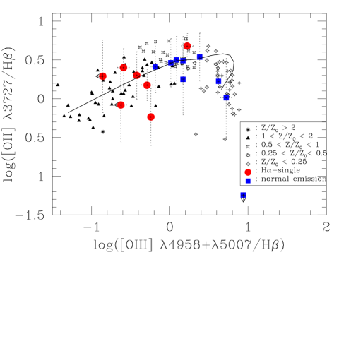
Figure 8: The relations between [O ii]/H$\beta$ and [O iii]/H$\beta$ in the “CFRS H$\alpha$-single” galaxies ($filled\leavevmode\nobreak\ circles$) and the “CFRS normal emission line” galaxies ($filled\leavevmode\nobreak\ squares$), together with a sample of the local H II regions and H II galaxies with different metallicities. The solid line shows the theoretical sequence from McCall et al. (MR85 (1985)), which fits the local H II galaxies well, with metallicity decreasing from the left to the right (also see Hammer et al. hammer97 (1997)).

5.3 Oxygen and nitrogen abundances

Oxygen is one of the main coolants in the nebular occurring primarily either via fine-structure lines in the far-infrared (52 and 88 $\mu$m) when the electron temperature is low or via forbidden lines in the optical ([O ii] $\lambda{3727}$, [O iii] $\lambda{4958}$ and [O iii] $\lambda{5007}$) when the electron temperature is high.

Given the absence of reliable [O iii] $\lambda{4363}$ detection, which is too weak to be measure except in extreme metal-poor galaxies, to derive the electron temperature of the ionized medium by comparing with [O iii] $\lambda\lambda{4958,5007}$ lines (Osterbrock 1989), oxygen abundances may also be determined from the ratio of [O ii]+[O iii] to H$\beta$ lines (“strong line” method). The general parameter is $R_{23}$: $R_{23}=({[O\textsc{ii]}}\lambda{3727}+{[O\textsc{iii]}}\lambda{4958}+{[O\textsc{iii]}}\lambda{5007})/H\beta$. To convert $R_{23}$ into 12+log(O/H), we adopt the analytical approximation given by Zaritsky et al. (ZKH94 (1994)) (hereafter ZKH), which is consistent with other calibration relations (see Kobulnicky & Zaritsky 1999, KZ99), and that is itself a polynomial fit to the average of three earlier calibrations for metal rich H II regions. This relationship has been used for all the galaxies except for CFRS14.1103 which presents a very small [O ii]/$H\beta$ ratio and no [N ii] $\lambda\lambda{6548,6583}$ and [S ii] $\lambda\lambda{6716,6731}$ emission lines are detected which characterize a low oxygen abundance medium, and for which we adopt the relation from Kobulnicky et al. (1999) for metal-poor branch galaxies. Its derived abundance by us is very similar to that of Tresse et al. (TH93 (1993)).

The derived oxygen abundances of the sample galaxies are given in Table 4 as 12+log(O/H), which are consistent with the results of Fig. 8. The “CFRS H$\alpha$-single” galaxies have larger abundance values than those of “CFRS normal emission line” galaxies, and lie in a region occupied by over-solar abundance objects, except for CFRS03.0578.

Figure 9 shows the oxygen abundance vs. absolute blue magnitude $M_{B}$ relations for the sample galaxies. It shows that the “CFRS H$\alpha$-single” galaxies are lying in the top metallicity area of local spiral galaxies and Emission Line Galaxies (ELGs) at $z=0.1\sim 0.5$ studied by KZ99, and the “CFRS normal emission line” galaxies are very similar to the local spiral galaxies except CFRS14.1103. The general trend of the sample galaxies follows: the brighter galaxies are more metal-rich. The Solar oxygen abundance (12+log(O/H)_⊙=8.83) was taken from Grevesse & Sauval (GS98 (1998)).

[N ii] $\lambda$6583 can be used in conjunction with [O ii] $\lambda$3727 and the temperature in the [N ii] emission regions (t${}_{{[N\textsc{ii]}}}$) to estimate the N/O ratio in the sample galaxies assuming $\frac{\rm N}{\rm O}=\frac{\rm N^{+}}{\rm O^{+}}$. Uncertainties due to emission line measurements, reddening and sky subtraction in the presence of strong night sky emission lines near [N ii] dominate the error budget for N/O.

First, we use the formula given by Thurston et al. (TEH96 (1996)) to estimate the temperature in the [N ii] emission region (t${}_{{[N\textsc{ii]}}}$) by using log$R_{23}$. Then, log(N/O) is estimated from ([N ii] $\lambda{6548}+\lambda{6583}$)/([O ii] $\lambda{3727}$) emission ratio and t${}_{{[N\textsc{ii]}}}$. The derived values are given in Table 4. Fig. 10 gives the log(N/O) vs. 12+log(O/H) relations for these sample galaxies. Most of them follow the $secondary$ nitrogen production well (Vila-Costas & Edmunds VilaE93 (1993)).

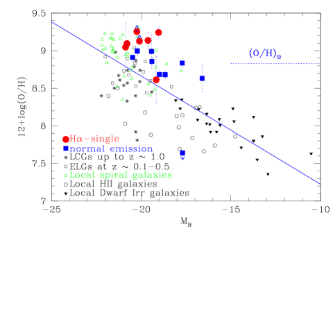
Figure 9: Oxygen abundances vs. absolute blue magnitudes for the “CFRS H$\alpha$-single” galaxies ($filled\leavevmode\nobreak\ circles$) and the “CFRS normal emission line” galaxies ($filled\leavevmode\nobreak\ squares$), associated with the Luminous Compact Galaxies (LCGs) up to $z$$\sim$1.0 ($asterisks$, from Gruel Gruel02 (2002) and Hammer et al. hammer01 (2001)), the Emission Line Galaxies (ELGs) at $z$$\sim$0.1-0.5 ($open$ $squares$, from Kobulnicky & Zaritsky KZ99 (1999): KZ99), the Local Spiral Galaxies ($open$ $triangles$, from ZKH), the Local H II Galaxies ($open\leavevmode\nobreak\ circles$, from Telles & Terlevich TT971 (1997)) and the Local Dwarf Irregular Galaxies ($upside-down$ $filled$ $triangles$, from Richer & McCall RM95 (1995)). All of them have been done using a spectral resolution comparable to ours. The solid line is a linear least-squares fit to local irregular and spiral galaxies (from KZ99). Solar oxygen abundance is shown by the dotted line.

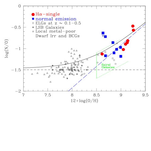
Figure 10: N/O vs. O/H relations for the “CFRS H$\alpha$-single” galaxies ($filled\leavevmode\nobreak\ circles$) and the “CFRS normal emission line” galaxies ($filled\leavevmode\nobreak\ squares$), associated with the ELGs at $z$$\sim$0.1-0.5 ($open$ $squares$, from KZ99), the Low Surface Brightness (LSB) Galaxies ($asterisks$, from van Zee et al. Zee97 (1997)), the Local metal-poor Dwarf Irregular and Blue Compact Galaxies (BCGs) ($open$ $triangles$, from Kobulnicky & Skillman KS96 (1996) and Izotov & Thuan IT99 (1999)). All of them have been done using a spectral resolution comparable to ours. The dotted box for spiral galaxies is taken from KZ99. The horizontal dot-dashed line refers to the $primary$ origin of nitrogen, the sloping dashed line refers to the $secondary$ origin, and the solid line is the combined contribution of a (delayed) $primary$ and a $secondary$ component of nitrogen (taken from Vila-Costas & Edmunds VilaE93 (1993)).

6 H$\alpha$ Luminosities and star formation rates

6.1 H$\alpha$ luminosities and SFRs

There is unique advantage at using H$\alpha$ to obtain the SFRs for low-$z$ galaxies. Among the Balmer lines, H$\alpha$ is the most directly proportional to the ionizing UV flux, and the weaker Balmer lines are much more affected by stellar absorption and reddening. The SFRs of the “CFRS H$\alpha$-single” galaxies were estimated from the H$\alpha$ luminosities.

In the following, we adopt Salpeter initial mass function (IMF) with low and high mass cutoffs at 0.1 and 100 $M_{\odot}$ (Salpeter Sal55 (1955)). The calibrations of Kennicutt et al. (K94 (1994)) and Madau et al. (Madau98 (1998)) yield:

$$SFR(M_{\odot}yr^{-1})=7.9\times 10^{-42}L(H\alpha)(ergs\leavevmode\nobreak\ s^{-1})\times Aper,$$ (2)

(Kennicutt K98 (1998)), with

$$L(H\alpha)=4\pi(3.086\times 10^{24}D_{L})^{2}f(H\alpha)(ergs\leavevmode\nobreak\ s^{-1}),$$ (3)

where $L(H\alpha)$ is the H$\alpha$ luminosity in ergs  s^-1, $f(H\alpha)$ is the integrated flux in ergs  s^-1 cm^-2 after correcting for the extinction, and $D_{L}$ is the luminosity distance in Mpc. $Aper$ is the aperture correction factor by comparing the photometric and spectral magnitudes in $I_{AB}$ band due to the limited size of the slit. The related results of these parameters and the derived SFRs are given in the left part of Table 5 (Col.(1)-(5)), in which Flux_c(H$\alpha$) is the H$\alpha$ emission flux after correcting for the extinction. CFRS galaxies have SFRs ranging from Milky Way value to higher typical values of starburst galaxies.

Table 5: Some derived characteristic parameters of the “CFRS H$\alpha$-single” (the top seven) and the “CFRS normal emission line” (the bottom nine) galaxies, the left part displays the results derived from the higher resolution spectra from the VLT or the CFHT, and the right part displays the results from low resolution CFRS spectra. The sequent columns in the right part of the table show the measured fluxes of (H$\alpha$+[N ii]) emission line, the rest-frame EW values of (H$\alpha$+[N ii]) emission line (in units of Å), the $N_{2}$ parameter, the measured fluxes of H$\beta$, the aperture correction factor, the SFRs with the average extinction $A_{V}=1$ (SFR₁), the estimated $A_{V}$ from the CFRS spectra (quoted as $A_{VC}$) and the derived SFRs by using $A_{VC}$ (SFR_C). All fluxes of the lines are given in units of (10^-17 ergs cm^-2 s^-1). All SFRs are in units of ($M_{\odot}$ $yr^{-1}$)

	Moderate		resolution				Very	low	resolution
	VLT	or	CFHT					CFRS
CFRS	Fluxc	Aper	L(H$\alpha$)	SFR	Flux	REW	$N_{2}$	Flux	Aper:	SFR1	$A_{VC}$	SFRC
	(H$\alpha$)		ergs s-1	M${}_{\odot}yr^{-1}$	(H$\alpha$+ [N ii])			(H$\beta$)	100.4a	$A_{V}$=1
(1)	(2)	(3)	(4)	(5)	(6)	(7)	(8)	(9)	(10)	(11)	(12)	(13)
03.0364	608.9$\pm{100.8}$	2.14	1042.26	31.22$\pm{5.17}$	94.8	44.5	0.42	0.0	2.14	7.52	—	—
03.0365	491.3$\pm{102.3}$	1.92	1042.04	16.84$\pm{3.50}$	121.8	52.6	0.36	0.0	1.49	5.22	—	—
03.0578	50.1$\pm{20.2}$	3.39	1041.11	3.48$\pm{1.23}$	18.9	46.8	0.42	0.0	2.03	1.05	—	—
03.0641	27.7$\pm{8.0}$	1.51	1040.96	1.08$\pm{0.31}$	25.5	20.5	0.45	0.0	1.50	1.50	—	—
03.0711	15.2$\pm{1.82}$	1.37	1040.70	0.54$\pm{0.06}$	14.4	32.9	0.45	0.0	1.28	0.73	—	—
03.1014	299.6$\pm{97.7}$	4.58	1041.73	19.60$\pm{6.40}$	103.8	24.7	0.45	0.0	1.89	4.24	—	—
22.0717	271.2$\pm{85.2}$	1.15	1042.01	9.31$\pm{2.93}$	19.5	10.8	0.54	—	1.41	1.17	—	—
03.0003	21.0$\pm{4.5}$	3.38	1040.68	1.27$\pm{0.27}$	8.2	95.0	0.21	1.7	1.22	0.34	0.90	0.21
03.0160	12.9$\pm{3.3}$	0.77	1040.47	0.18$\pm{0.05}$	16.9	38.9	0.45	1.2	0.77	0.35	3.13	1.99
03.0149	27.7$\pm{4.1}$	2.87	1040.92	1.90$\pm{0.28}$	17.8	51.0	0.36	3.2	2.56	1.76	0.91	1.67
03.1299	1442.1$\pm{281.0}$	2.28	1042.31	37.18$\pm{7.24}$	224.0	77.0	0.36	16.1	2.28	9.33	3.25	58.2
03.1311	531.2$\pm{88.0}$	1.77	1041.88	10.68$\pm{1.77}$	69.5	41.6	0.45	2.7	1.77	2.12	4.66	41.0
14.1103	133.9$\pm{3.0}$	2.08	1041.44	4.50$\pm{0.10}$	97.7	2434.0	0.15	39.0	2.08	—	0.00	2.86
14.1117	16.0$\pm{2.8}$	4.73	1040.44	1.03$\pm{0.18}$	19.6	69.0	0.36	4.7	4.73	2.04	0.18	1.07
22.0474	102.7$\pm{10.9}$	1.10	1041.59	3.40$\pm{0.36}$	53.5	312.0	0.15	10.4	1.54	4.77	1.14	5.40
22.1084	89.8$\pm{20.8}$	1.73	1041.57	5.15$\pm{1.32}$	31.5	37.7	0.45	2.3	1.73	2.74	3.05	14.5

6.2 Comparing the SFRs with those from low-resolution CFRS spectra

To understand more the effect of spectral resolution on the derived SFRs, we also estimated the SFRs of these galaxies from their low-resolution CFRS spectra. For the latter estimates, we have followed the method suggested by TM98 and used the extinction law from Osterbrock (1989), then the dereddened and aperture corrected H$\alpha$ fluxes are estimated by:

$$f(H{\alpha})=\frac{f(H{\alpha}+{[N\textsc{ii]}})}{1+N_{2}}10^{c(1.13-0.37)}10^{0.4a},$$ (4)

where $c=A_{V}\times 1.47/3.2$ (see Sect.4). For the seven“CFRS H$\alpha$-single” galaxies, extinction cannot be estimated from Balmer decrement due to the absence of H$\beta$ emission, we use the average $A_{V}=1$, corresponding to $c=0.45$, by following TM98. $N_{2}$ is the parameter to reflect [N ii] $\lambda$6583 emission mixed with H$\alpha$ in the CFRS spectra. We got $N_{2}$ values from Fig. 3(b) of TM98 by considering the rest-frame EW(H$\alpha$+[N ii]). $a$ refers to the aperture correction factor by comparing the photometric and spectral magnitudes in $V_{AB}$ band. Corresponding values are given in the right part of Table 5 (Col.(6)-(13)).

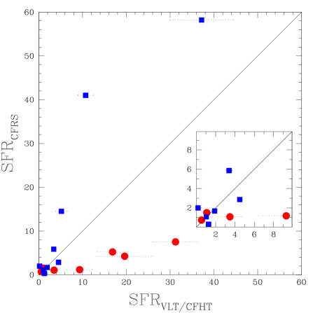
Figure 11: Comparison between the SFRs of the sample galaxies obtained from the low-resolution CFRS spectra (SFR_CFRS) and the higher quality spectra (SFR_VLT/CFHT) studied in this work. The small figure on this figure shows the detail around the origin. For SFR_CFRS, SFR₁ were used for the seven “CFRS H$\alpha$-single” galaxies, and SFR_C were used for the nine “CFRS normal emission line” galaxies (see Table 5). Symbols as in Fig. 1.

Figure 11 shows how misleading are the SFR estimates based on low resolution spectra by comparing the corresponding SFR_CFRS with the SFR_VLT/CFHT from the moderate resolution spectra. Thus, it may be that TM98 systematically underestimated the SFRs of the “CFRS H$\alpha$-single” galaxies simply because they underestimated the actual extinction coefficients of these galaxies. Conversely, the SFRs of “CFRS normal emission line” galaxies are often overestimated since the underlying absorption beneath $H\beta$ could not be properly accounted for in low resolution spectroscopy and leads to a severe overestimation of the extinction coefficient properties. This effect probably generates the derived $A_{V}$ values exceeding 3 or 4 (see Table 5, also Tresse et al. 1996). SFRs of individual galaxies can be only recovered by a proper analysis of the higher quality spectra (SFR_VLT/CFHT) at moderate spectral resolution.

6.3 Estimates of Cosmic Star Formation Density (CSFD)

From the above, some qualitative arguments can be used to test the validity of previous works based on low resolution spectroscopy or narrow band filter imagery. Although the latter cannot provide quantitative SFR measurements of individual galaxies, it is valuable to notice that, the SFR overestimates and underestimates are almost balanced in the TM98 study (Fig. 11). Table 6 report the total SFR budget assuming that the seven “CFRS H$\alpha$-single” galaxies and the nine “CFRS normal emission line” galaxies are the representative of the whole CFRS sample at low redshift. The difference between the two estimates is only 13% which is far below the error bars in TM98. Table 5 shows the extinction coefficients of “CFRS normal emission line” galaxies could be much overestimated from the very low resolution spectroscopy. If unrealistic values of $A_{V}$ ($\geq$3.5) are taken to calculate the SFRs of these galaxies, hence the SF density, this could lead to severe overestimations. Recall that for the luminous infrared galaxies, Flores et al. (2003) never find $A_{V}$ values larger than 3.5. And the average color excesses, $E(B-V)$, of luminous infrared galaxies (LIGs) studied by Veilleux et al. (VK95 (1995)) are only 0.72, 0.99 and 1.14 in Seyfert 2, H II LIGs and LINERs, respectively.

Fujita et al. (2003) have corrected their $H\alpha$ luminosities from narrow band filter imagery using $A_{H\alpha}$= 1 which grossly corresponds to $A_{V}$ $\sim$ 1.25. This value is in agreement with our median value for the 16 galaxies studied here. However this correction is related to the power law of the extinction coefficient, leading to important effect related to the large extinction coefficients. Table 7 compares the effect of applying the Fujita et al. (2003) correction on the 16 galaxies studied here. The result is that Fujita et al. (2003) might have underestimated their SF density by a factor close to 2.

It is out of the scope of this paper to provide a quantitative estimates of the CSFD, because of the small number of objects studied. Indeed, the study here would not help in reconciling the different estimates at low redshift. It however strongly calls for a systematic survey at moderate resolution of a complete sample of galaxies detected from deep narrow band imagery, in order to correct the $H\alpha$ luminosities by properly estimating the extinction coefficients.

Table 6: The comparison of the total SFRs (in units of $M_{\odot}$ $yr^{-1}$) for the CFRS low-$z$ sample. The adopted interstellar extinction law assumes ($f(H\alpha)-f(H\beta)$=$-$0.323) and the total galaxies are 110 here by following TM98

	Total SFRVLT/CFHT	Total SFRCFRS
57 “CFRS H$\alpha$-single” galaxies	696.5	160.3
53 “CFRS normal” galaxies	389.7	780.2
Total 110	1086.2	940.5

Table 7: The comparison of the SFRs (in units of $M_{\odot}$ $yr^{-1}$) of the 16 CFRS low-$z$ galaxies from different extinctions

	Total SFRsVLT/CFHT	Total SFRsVLT/CFHT
	with well determined $A_{V}$	assuming $A_{H\alpha}=1$
seven “CFRS H$\alpha$-single” galaxies	82.1	31.4
nine “CFRS normal” galaxies	65.3	43.4
Total 16	147.4	74.8

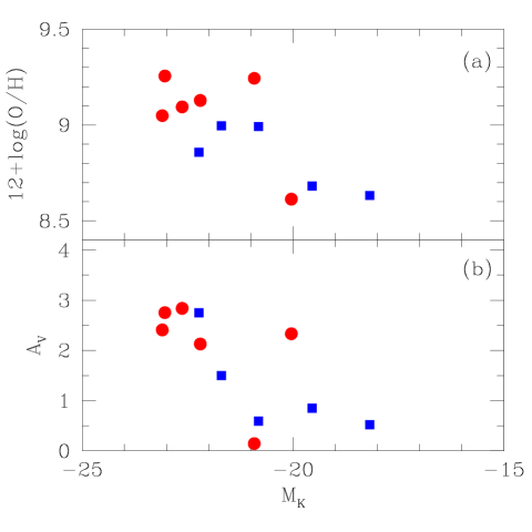
Figure 12: Oxygen abundances (top) and extinction coefficients (bottom) against absolute K band magnitudes for the sample galaxies. Both relations show the trends that the higher abundances and extinctions are in the more massive stellar systems. Symbols as in Fig. 1.

7 Discussion and conclusion

Using moderately high resolution (R$>$600) and high S/N spectra obtained from the VLT and the CFHT, we have studied the properties of a sample of 16 CFRS low redshift galaxies. This sample could be splitted in seven “CFRS H$\alpha$-single” emission galaxies, and nine “CFRS normal emission line” galaxies, from their spectral properties at the CFRS very low spectral resolution. Selected from the CFRS sample, these can be taken as representative of the H$\alpha$-emission field galaxy population at $z$$\leq$0.3.

Using the Balmer decrement method (H$\alpha$ to H$\beta$), we have been able to calculate their interstellar extinction values, by properly accounting for the underlying stellar absorption.

Two diagnostic diagrams (log([O iii] $\lambda{5007}$/H$\beta$) vs. log([N ii] $\lambda{6583}$/H$\alpha$) and log([O iii] $\lambda{5007}$/H$\beta$) vs. log([S ii] $\lambda 6716+\lambda{6731}$/H$\alpha$) have been obtained to derive firm conclusion about the nature of the emission line activity, especially because that [N ii] emission lines are divided from H$\alpha$ emission in these higher resolution spectra. Derivation of extinction properties have allowed to accurately estimate their oxygen and nitrogen abundances, as well as to calculate their SFRs using the extinction corrected H$\alpha$ luminosities.

We find that the spectral properties of galaxies at very low spectral resolution can be well understood by the properties of their interstellar media. Namely “CFRS H$\alpha$-single emission” galaxies shows systematically larger extinction coefficient, higher oxygen and nitrogen abundances than the rest of the sample. These properties suffice to explain why $H\beta$ and [O iii] $\lambda$5007 emissions are undetected by low resolution spectroscopy. They can be considered to be the mature and massive spirals that lie at low redshifts as it can be derived from their K absolute magnitudes (Fig.12).

SFRs of these low redshift galaxies are ranging from 0.5 $M_{\odot}$ $yr^{-1}$ (Milky Way value) to 40 $M_{\odot}$ $yr^{-1}$ (strong starburst). We also find that the SFRs of individual galaxies cannot be properly derived using low resolution spectroscopy. Indeed, extinction corrections are often large and requires a proper account of the underlying stellar absorption to the Balmer lines, which is simply impossible at spectral resolution lower than 600. Previous studies of SF density at low redshifts have assumed average properties for underlying absorption or even for extinction of Balmer line fluxes derived from low resolution spectroscopy. Indeed, $H\beta$ line is affected by underlying absorption and extinction in such a complex way that only moderate resolution can estimate properly the $H\alpha/H\beta$ ratio. Hence, the previous studies may systematically underestimated the contribution of “CFRS H$\alpha$-single” emission galaxies (the mature and massive systems) and overestimated the contribution of other normal emission line galaxies.

From the data shown here, one can only speculate about the consequences at higher redshifts. Deep surveys preferentially select luminous galaxies in their highest redshift bins, which generally show relatively large extinction coefficients (see Fig. 12). This effect may explain most of the $\sim$60% gap between the SF density derived by Tresse et al. (2002) (from $H\alpha$ luminosity, assuming $A_{V}$= 1) and that of Flores et al. (1999) (from combination of IR and UV measurements). Indeed, in a forthcoming paper, Flores et al. (2004, in preparation) find that one third of the Tresse et al.’s sample are luminous infrared galaxies, for which $A_{V}$ should reach values much larger than 1.

The present study gives a obvious warning for the studies based on low resolution spectroscopy aimed at measuring individual galaxy properties (gas chemical abundances, interstellar extinction, stellar population, ages as well as star formation rates and history), particularly for the metal rich and dusty spiral galaxies. Because this affects a large fraction of the galaxies, deriving cosmological star formation density from low resolution spectroscopic surveys could lead to severe biases.

References

- (1) Crampton, D., Le Fèvre, O., Lilly, S. J., Hammer, F., 1995, ApJ 455, 96 (CFRS V)
- (2) Flores, H., Hammer, F. et al. 2004 (in preparation)
- (3) Flores, H., Hammer, F., Elbaz, D. et al. 2003, A&A (in press), astro-ph/0311113
- (4) Flores, H., Hammer, F, Thuan, T. X. et al. 1999, ApJ 517, 148
- (5) Fujita, S. S., Ajiki, M., Shioya, Y., et al. 2003, ApJL 586, L115
- (6) Giovanelli, R., Haynes, M. P., Salzer, J. J. et al. 1995, AJ 110, 1059
- (7) Grevesse, N. & Sauval, A. J. 1998, Space Sci. Rev. 85, 161
- (8) Gruel, N. PhD thesis (http:// girafdb.obspm.fr/lirgsiso)
- (9) Gruel, N., Hammer F., Flores, H. et al. 2003 (in preparation)
- (10) Hammer, F., Crampton, D., Le Fèvre, O. et al. 1995, ApJ 455, 88 (CFRS IV)
- (11) Hammer, F. & Flores, H., Proceedings of the meeting held in Lyon, France, May 28-June 1st, 2001, Eds.: F. Combes, D. Barret, F. Thévenin, to be published by EdP-Sciences, Conference Series, p.251
- (12) Hammer, F., Gruel, N., Thuan, T. X. et al. 2001, ApJ 550, 570
- (13) Hammer, F., Le Fèvre, O., Lilly, S. J. et al. 1997, ApJ 481, 49 (CFRS XIV)
- (14) Izotov, Y. I., Thuan, T. X. 1999, ApJ 511, 639
- (15) Jacoby, G. H., Hunter, D. A., Christian, C. A., 1984, ApJS 56, 257
- (16) Kennicutt, R. C., Jr. 1998, ARA&A 36, 189
- (17) Kennicutt, R. C., Jr., Tamblyn, P., Congdon, C. W. 1994, ApJ 435, 22
- (18) Kent, S. M. 1985, ApJS 59, 115
- (19) Kobulnicky, H. A., Kennicutt, R. C., Jr., Pizagno, J. L. 1999, ApJ 514, 544
- (20) Kobulnicky, H. A., Skillman, E. D. 1996, ApJ 471, 211
- (21) Kobulnicky, H. A., Zaritsky, D. 1999, ApJ 511, 118 (KZ99)
- (22) Le Fèvre, O., Crampton, D., Lilly, S. J. et al. 1995, ApJ 455, 60 (CFRS II)
- (23) Lilly, S. J., Le Fèvre, O., Crampton, D. et al. 1995a, ApJ 455, 50 (CFRS I)
- (24) Lilly, S. J., Hammer, H., Le Fèvre, O. et al. 1995b, ApJ 455, 75 (CFRS III)
- (25) Lilly, S. J., Schade, D., Le Fèvre, O. et al. 1998, ApJ 500, 75
- (26) Madau, P., Pozzetti, L., Dickinson, M. 1998, ApJ 498, 106
- (27) McCall, M. L., Rybski, P. M., Shields, G. A. 1985, ApJS 57, 1
- (28) Osterbrock , D. E. Astrophysics of Gaseous Nebulae and Active Galactic Nuclei. Mill Valley, California: University Science Books, 1989
- (29) Pascual, S., Gallego, J., Aragon-Salamanca, A. et al. 2001, A&A 379, 798
- (30) Richer, M. G., McCall, M. L., 1995 ApJ 445, 642
- (31) Salpeter, E. E. ApJ 1955, 121, 161
- (32) Seaton, M. J. 1979, MNRAS 187, 73
- (33) Simard, L., Willmer, C. N. A., Vogt, N. P. et al. 2002, ApJS 142, 1
- (34) Telles, E., Terlevich, R. 1997, MNRAS 286, 183
- (35) Thurston, T. R., Edmunds, M. G., Henry, R. B. C. 1996, MNRAS 283, 990
- (36) Tresse, L., Hammer, F., Le Fèvre, O. et al. 1993, A&A 277, 53
- (37) Tresse, L., Maddox, S. J. 1998, ApJ 495, 691 (TM98)
- (38) Tresse, L., Maddox, S. J., Le Fèvre, O., Cuby, J.-G, 2002, MNRAS 337, 369
- (39) Tresse, L., Rola, C., Hammer, F. et al. 1996, MNRAS 281, 847 (CFRS XII)
- (40) van Zee, L., Haynes, M. P., Salzer, J. J. 1997, AJ 114, 2479
- (41) van Zee, L., Salzer, J. J., Haynes, M. P. et al. 1998, AJ 116, 2805
- (42) Vila-Costas, M. B. & Edmunds, M. G. 1993, MNRAS 265, 119
- (43) Veilleux, S., Kim, D.-C., Sanders, D. B. et al. 1995 ApJS 98, 171
- (44) Veilleux, S., Osterbrock, D. E., 1987, ApJS 63, 195
- (45) Zaritsky, D., Kennicutt, R. C., Huchra, J. P. 1994, ApJ 420, 87 (ZKH)