Characteristic Angular Scales in Cosmic Microwave Background Radiation

Abstract

We investigate the stochasticity in temperature fluctuations in the cosmic microwave background (CMB) radiation data from Wilkinson Microwave Anisotropy Probe. We show that the angular fluctuations of the temperature is a Markov process with a Markov angular scale, $\Theta_{\rm Markov}=1.01^{+0.09}_{-0.07}$. We characterize the complexity of the CMB fluctuations by means of a Fokker-Planck or Langevin equation and measure the associated Kramers-Moyal coefficients for the fluctuating temperature field $T(\hat{n})$ and its increment, $\Delta T=T(\hat{n}_{1})-T(\hat{n}_{2})$. Through this method we show that temperature fluctuations in the CMB has fat tails compared to a Gaussian distribution.

Key Words: New applications of statistical mechanics

]

I Introduction

The Wilkinson Microwave Anisotropy Probe (WMAP) mission is one of the main experiments in the cosmic microwave background (CMB) that determines the power spectrum of the temperature fluctuations in the CMB with high accuracy. It has been shown that the universe is geometrically flat, and that the dominant content of the universe is an exotic dark energy which causes the expansion of the universe to be accelerated [1, 2, 3, 4]. The statistical properties of the CMB radiation is an important tool for identifying the appropriate cosmological model and determining the parameters of the standard model [5]. The traditional way of studying the CMB data is through analyzing their angular power spectrum and computing the two-point correlation function. In order to gain full statistical information from the temperature fluctuations on the last scattering surface, we should use the $n$-point joint probability density function (PDF) or the $n$-point correlation function.

At the same time, Gaussianity of the CMB anisotropy is an important question which is linked with the theoretical predictions made by the inflationary cosmology [6, 7, 8]. With current developments in experimental CMB physics, we are now in a position to analyze very large data sets that provide information about large patches of the sky, measured with very high resolution and sensitivity. This means that we can precisely test whether the CMB is Gaussian. Tantalizing evidence of non-Gaussianity has been emerging in the WMAP sky maps, using a variety of methods. The statistical properties of the primordial fluctuations generated by the inflationary cosmology are closely related to the anisotropy of the CMB radiation. Thus, measurement of the possible non-Gaussianity of the CMB data is a direct test of the inflation paradigm. If the CMB anisotropy is Gaussian, then the angular power spectrum, or the two-point correlation function, fully specifies its statistical properties.

In this paper we study the statistical properties of the CMB anisotropy through the $n$-point joint PDF of temperature fluctuations in the CMB data. We show that the fluctuations constitute a Markovian process with a Markov angular scale of $\Theta_{\rm Markov}=1.01^{+0.09}_{-0.07}$, or in the Legendre space, $l_{\rm Markov}=178.22^{+0.27}_{-0.21}$, at $1\sigma$ confidence level. Using the Markov properties of the CMB data, a master equation for the angular evolution of the probability distribution function - the Fokker-Planck (FP) equation - is obtained. To derive the relation between the standard power-spectral analysis and the Markov properties of the CMB data, we consider the joint probability distribution $P(T_{2},\hat{n}_{2};T_{1},\hat{n}_{1})$ that describes the probability of finding simultaneously $T_{1}$ in the direction, $\hat{n}_{1}=(\theta_{1},\phi_{1})$, and $T_{2}$ in the direction $\hat{n}_{2}=(\theta_{2},\phi_{2})$. We then evaluate the corresponding Kramers-Moyal (KM) coefficients, and compute the first and second KM coefficients (i.e., the drift and diffusion coefficients in the FP equation). We show that the higher-order coefficients in the KM expansion are very small and can be ignored. In addition, using the FP equation for the PDF, we show that temperature fluctuations on the last scattering surface are consistent with a Gaussian distribution. We also use the same analysis to investigate temperature fluctuations in the northern and southern hemispheres. The analysis detects some cold and hot spots in the southern and northern hemisphere, respectively.

The organization of this paper is as follows: In Section II we determine the 2-point joint PDF of temperature fluctuations and obtain the correlation angular scale. In Section III we introduce the mathematical property of the PDF for the Markovian process and obtain the Markov angular scale for the WMAP data. We also develop the master equation in the form of a FP equation for the CMB data. In Section IV we investigate the (non)-Gaussian nature of the temperature fluctuations in the CMB. The relation between the Markov and the angular power spectrum for this set of data is obtained in Section V. The conclusions are presented in Section VI.

FIG. 1.: The arbitrary directions $\hat{n}_{0}$, $\hat{n}_{1}$ and $\hat{n}_{2}$ in the sky to the last scattering surface.

FIG. 2.: $\Theta$ is the angular separation between two directions $\hat{n}_{1}$ and $\hat{n}_{2}$. For $\Theta_{C}=24.86^{o}\pm 0.03$ we obtain the minimum value for the $\Delta P(T_{2},T_{1})=|P(T_{2},\hat{n}_{2};T_{1},\hat{n}_{1})-P(T_{1},\hat{n}_{1})P(T_{2},\hat{n}_{2})|$ vs $\Theta$.

II Correlation angular scale by the joint PDF decomposition analysis

The WMAP instrument is composed of 10 differencing assemblies, spanning five frequencies from 23 to 94 GHz [9]. The two lowest frequency bands (K and Ka) are primarily galactic foreground monitors, while the three highest (Q, V, and W) are primarily cosmological bands. The full width at half-maximum for the detectors is a function of the frequency and ranges from $0.82^{\circ}$ at 23 GHz to $0.21^{\circ}$ at 94 GHz [10]. Here, we use the Internal Linear Combination Map which is a weighted linear combination of the five WMAP frequency maps. The weights are computed using the criterion that minimize the galactic foreground contribution to the sky signal. The resultant map provides a low-contamination image of the CMB anisotropy.

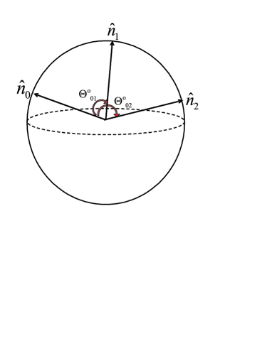
Let the temperature fluctuation in the CMB data in the direction of $\hat{n}=(\theta,\phi)$ be represented by ${\cal T}(\hat{n})$, and define $T(\hat{n})\equiv({\cal T}(\hat{n})-\bar{T})/\sigma$, where $\bar{T}$ and $\sigma$ are the mean and variance of the temperature fluctuations, respectively. For a direction $\hat{n}_{0}$ with $T(\hat{n}_{0})=T_{0}$, at any $\hat{n}\neq\hat{n}_{0}$, $T(\hat{n})$ is given by a PDF $P(T,\hat{n})$ (see figure 1). This means that $T(\hat{n})$ for $\hat{n}\neq\hat{n}_{0}$ is a stochastic (and possibly correlated) variable.

Complete information about the stochastic process is obtained from the knowledge about all the possible $k$-point or, more precisely, $k$-scale joint PDF (JPDF), $P(T_{k},\hat{n}_{k};T_{k-1},\hat{n}_{k-1};...;T_{1},\hat{n}_{1})$, describing the probability of finding simultaneously, $T_{1}$ in the direction $\hat{n}_{1}$, $T_{2}$ in the direction $\hat{n}_{2}$, and so on up to $T_{k}$ on the direction $\hat{n}_{k}$. Moreover, we can define the conditional probability distribution function. For a given $T(\hat{n}_{0})=T_{0}$, the conditional probability of $T(\hat{n})$ at the successive positions $\hat{n}_{1},\hat{n}_{2},\cdots,\hat{n}_{k}$, to be $T(\hat{n}_{1}),T(\hat{n}_{2}),\cdots,T(\hat{n}_{k})$ is described by

$$P_{k}^{1}(T_{k},\hat{n}_{k};\cdots;T_{1},\hat{n}_{1}|T_{0},\hat{n}_{0})dT_{k}dT_{k-1}\cdots dT_{1}=$$ (1)

$${\rm Prob}\{T(\hat{n}_{i})\in[T_{i},T_{i}+dT_{i}]\hskip 5.69046pt$$ (2)

$${\rm for}\hskip 5.69046pti=1,2,\cdots k\hskip 5.69046pt{\rm and}\hskip 5.69046ptT(\hat{n}_{0})=T_{0}\}.$$ (3)

In this notation, the superscript (for the $P$) represents the number of conditions (e.g., here, we have one condition), while the subscript denotes the number of stochastic variables in the joint PDF. The $k$-point JPDF of the temperature fluctuations is expressed by the product of the multiconditional PDFs as

$$P(T_{k-1},\hat{n}_{k-1};T_{k-2},\hat{n}_{k-2};...;T_{1},\hat{n}_{1};T_{0},\hat{n}_{0})=$$ (4)

$$P_{1}^{k-1}(T_{k-1},\hat{n}_{k-1}|T_{k-2},\hat{n}_{k-2};...;T_{1},\hat{n}_{1};T_{0},\hat{n}_{0})$$ (5)

$$\times P_{1}^{k-2}(T_{k-2},\hat{n}_{k-2}|T_{k-3},\hat{n}_{k-3};...;T_{1},\hat{n}_{1};T_{0},\hat{n}_{0})$$ (6)

$$\times...P_{1}^{1}(T_{1},\hat{n}_{1}|T_{0},\hat{n}_{0})P(T_{0},\hat{n}_{0})~{}.$$ (7)

where, $P_{1}^{1}(T_{1},\hat{n}_{1}|T_{0},\hat{n}_{0})$ denotes a conditional probability of finding temperature fluctuation $T_{1}$ in the direction $\hat{n}_{1}$, under the condition that the temperature $T_{0}$ in the direction $\hat{n}_{0}$ has been found. This conditional probability can be expressed by 2-point JPDF, as: $P_{1}^{1}(T_{1},\hat{n}_{1}|T_{0},\hat{n}_{0})=\frac{P(T_{1},\hat{n}_{1};T_{0},\hat{n}_{0})}{P(T_{0},\hat{n}_{0})}$, this result is important because, if the conditional PDF for the $T_{1}$ is independent of $T_{0}$, then $P_{1}^{1}(T_{1},\hat{n}_{1}|T_{0},\hat{n}_{0})=P(T_{1},\hat{n}_{1})$, in this case: $P_{1}^{1}(T_{1},\hat{n}_{1};T_{0},\hat{n}_{0})=P(T_{1},\hat{n}_{1})P(T_{0},\hat{n}_{0})$.

To derive the first characteristic angular scales in the CMB, we define the correlation angular scale, where the JPDF can be decomposed into the production of two independent PDFs [11] as

$$P(T_{2},\hat{n}_{2};T_{1},\hat{n}_{1})|_{\Theta_{C}}=P(T_{1},\hat{n}_{1})P(T_{2},\hat{n}_{2}).$$ (8)

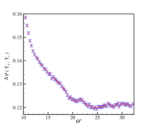
Here, $\Theta$ is the angular separation between the two direction $\hat{n}_{1}$ and $\hat{n}_{2}$, and we assumed the statistical isotropy of the temperature fluctuations in the CMB in which the correlation function depends only on the angle between the two directions of $\hat{n}_{1}$ and $\hat{n}_{2}$ [12]. In Fig. 2 we plot $\Delta P(T_{2},T_{1})=|P(T_{2},\hat{n}_{2};T_{1},\hat{n}_{1})-P(T_{1},\hat{n}_{1})P(T_{2},\hat{n}_{2})|$ in terms of $\Theta$, using the least square method,

$$\chi^{2}=\int\frac{[P(T_{2},\hat{n}_{2};T_{1},\hat{n}_{1})-P(T_{1},\hat{n}_{1})P(T_{2},\hat{n}_{2})]^{2}}{\sigma_{PDF}^{2}+\sigma_{2-{\rm joint}}^{2}}dT_{1}dT_{2},$$ (9)

where the minimum value of $\chi^{2}$ corresponds to the angular scale, at which the correlation disappears. Here, $\sigma_{PDF}^{2}$ and $\sigma_{2-{\rm joint}}^{2}$ are the variance of $P(T_{1},\hat{n}_{1})P(T_{2},\hat{n}_{2})$ and $P(T_{2},\hat{n}_{2};T_{1},\hat{n}_{1})$, respectively. Our analysis indicates that the minimum value of $\Delta P(T_{2},T_{1})$ happens at the $\Theta_{C}=24.86^{o}\pm 0.03$ with $\chi^{2}_{\nu}=1.01$ ($\chi^{2}_{\nu}={\chi^{2}}/{\cal{N}}$, with $\cal{N}$ being the number of degree of freedom).

III CMB data as a Markov Process: Least Squares Test

Now, let us check whether the CMB data follow a Markov chain and, if so, measure the second characteristic angular scale in the CMB, i.e., the Markov angular scale $\Theta_{\rm Markov}$ - the scale over which the CMB data are Markov-correlated. In other words, the Markov angular scale $\Theta_{\rm Markov}$ is the minimum angular separation over which the data can be represented by a Markov process [13, 14, 15]. The exact mathematical definition of the Markov process is given [16] by

$$P(T_{k},\hat{n}_{k}|T_{k-1},\hat{n}_{k-1};\cdots;T_{1},\hat{n}_{1};T_{0},\hat{n}_{0})=$$ (10)

$$\qquad\qquad P(T_{k},\hat{n}_{k}|T_{k-1},\hat{n}_{k-1}).$$ (11)

Intuitively, the physical interpretation of a Markov process is that it ”forgets its past,” or, in other words, only the most nearby conditioning, say $(T_{k},n_{k})$, is relevant to the probability of finding a temperature $T_{k}$ at $n_{k}$. In the Markov process the ability to predict the value of $T(\hat{n})$ will not be enhanced by knowing its values in the steps prior to the most recent one. Therefore, an important simplification that can be made for a Markov process is that a conditional multivariate JPDF (Eq. 4) can be written in terms of the products of simple two-parameter conditional PDFs [16] as

$$P(T_{k},\hat{n}_{k};T_{k-1},\hat{n}_{k-1};\cdots;T_{1},\hat{n}_{1}|T_{0},\hat{n}_{0})=$$ (12)

$$\qquad\qquad\prod_{i=1}^{k}P(T_{i},\hat{n}_{i}|T_{i-1},\hat{n}_{i-1}).$$ (13)

In what follows, we use the least-square method to determine the Markov angular scale of the CMB temperature fluctuations. Testing Eq. (10) for large values of $k$ is out of our computational capability; however, for $k=3$, where we have three vectors pointing the 2D celestial sphere, the Markov condition is as follows,

$$P(T_{3},\hat{n}_{3}|T_{2},\hat{n}_{2};T_{1},\hat{n}_{1})=P(T_{3},\hat{n}_{3}|T_{2},\hat{n}_{2}),$$ (14)

where $\Theta_{ij}=\arccos(\hat{n}_{i}.\hat{n}_{j})$ is the separation angle of $\hat{n}_{i}$ and $\hat{n}_{j}$ and $\Theta_{31}>\Theta_{32},\Theta_{21}$ (see Fig. 1). For simplicity, we let $\Theta_{21}=\Theta_{32}$. A process is Markovian if Eq. (14) is satisfied for a certain angular separation which, in our notation, is $\Theta_{32}$. We refer to it as the Markov angular scale $\Theta_{\rm Markov}$).

In order to determine the Markov angular scale, we compare the three-point PDF with that obtained based on the Markov process. The three-point PDF, in terms of conditional probability functions, is given by

$$P(T_{3},\hat{n}_{3};T_{2},\hat{n}_{2};T_{1},\hat{n}_{1})=$$ (15)

$$\qquad P(T_{3},\hat{n}_{3}|T_{2},\hat{n}_{2};T_{1},\hat{n}_{1})P(T_{2},\hat{n}_{2};T_{1},\hat{n}_{1}).$$ (16)

Using the properties of the Markov process and substituting Eq. (14) we obtain:

$$P_{Mar}(T_{3},\hat{n}_{3};T_{2},\hat{n}_{2};T_{1},\hat{n}_{1})=$$ (18)

$$\qquad P(T_{3},\hat{n}_{3}|T_{2},\hat{n}_{2})P(T_{2},\hat{n}_{2};T_{1},\hat{n}_{1}).$$

In order to check the condition for the data being a Markov process, we must compute the three-point JPDF through Eq. (15) and compare the result with Eq. (18). The first step in this direction is to determine the quality of the fit through the least-squared fitting quantity $\chi^{2}$ defined by

$$\chi^{2}=\int dT_{3}dT_{2}dT_{1}[P(T_{3},\hat{n}_{3};T_{2},\hat{n}_{2};T_{1},\hat{n}_{1})$$ (19)

$$-P_{\rm Mar}(T_{3},\hat{n}_{3};T_{2},\hat{n}_{2};T_{1},\hat{n}_{1})]^{2}/\left[\sigma_{3-{\rm joint}}^{2}+\sigma_{\rm Mar}^{2}\right]$$ (20)

where $\sigma^{2}_{3-{\rm joint}}$ and $\sigma^{2}_{\rm Mar}$ are the variances of $P(T_{3},\hat{n}_{3};T_{2},\hat{n}_{2};T_{1},\hat{n}_{1})$ and $P_{\rm Mar}(T_{3},\hat{n}_{3};T_{2},\hat{n}_{2};T_{1},\hat{n}_{1})$, respectively. To compute the Markov angular scale, we use the Likelihood statistical analysis [17]. In the absence of a prior constraint, the probability of the set of three-points JPDF is given by a product of Gaussian functions:

$$p(\arccos(\hat{n}_{3},\hat{n}_{2}))=\prod_{T_{3},T_{2},T_{1}}\frac{1}{\sqrt{2\pi(\sigma_{3-{\rm joint}}^{2}+\sigma_{\rm Mar}^{2})}}$$ (21)

$$\exp[-\frac{[P(T_{3},\hat{n}_{3};T_{2},\hat{n}_{2};T_{1},\hat{n}_{1})-P_{\rm Mar}(T_{3},\hat{n}_{3};T_{2},\hat{n}_{2};T_{1},\hat{n}_{1})]^{2}}{2(\sigma_{3-{\rm joint}}^{2}+\sigma_{\rm Mar}^{2})}]$$ (22)

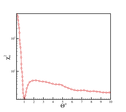
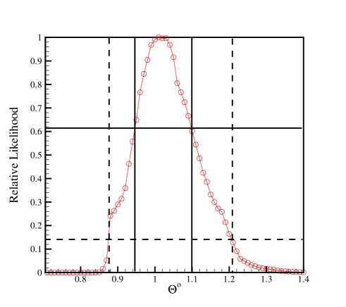
This probability distribution must be normalized. Evidently, when, for a set of values of the parameters, the $\chi^{2}$ is minimum the probability is maximum. Figure 3 shows the normalized $\chi^{2}_{\nu}$ as a function of the angular length scale $\Theta=\Theta_{32}\equiv\arccos(\hat{n}_{3}.\hat{n}_{2})$. The minimum value of $\chi^{2}_{\nu}$ is $1.38$, corresponding to $\Theta_{\rm Markov}=1.01^{+0.09}_{-0.07}$ with $1\sigma$ confidence level. Figure 4 shows the likelihood function of Markov angular scale of CMB.

FIG. 3.: $\chi^{2}_{\nu}$ in terms of angular scale $\Theta$. The minimum value of $\chi^{2}_{\nu}=1.388$ corresponds to $\Theta_{\rm Markov}=1.01^{+0.09}_{-0.07}$, with $1\sigma$ confidence level.

FIG. 4.: Relative likelihood function of the Markov angular scale of the CMB fluctuations, as a function of $\Theta^{\circ}$. The intersections of the curve with the horizontal solid and dashed lines give the bounds with $1\sigma$ and $2\sigma$ confidence levels, respectively. The minimum value of $\chi^{2}_{\nu}=1.38$ corresponds to $\Theta_{\rm Markov}=1.01^{+0.09}_{-0.07}$, with $1\sigma$ and $\Theta_{\rm Markov}=1.01^{+0.19}_{-0.13}$, with $2\sigma$ confidence level.

The Markov nature of the CMB enables us to derive a master equation - a FP equation - for the evolution of the PDF $P(T,\hat{n})$, in terms of, for example, the direction $\hat{n}$. One writes Eq. (8) as an integral equation, which is well-known as the Chapman-Kolmogorov (CK) equation:

$$P(T_{3},\hat{n}_{3}|T_{1},\hat{n}_{1})=\int dT_{2}\;P(T_{3},\hat{n}_{3}|T_{2},\hat{n}_{2})\;P(T_{2},\hat{n}_{2}|T_{1},\hat{n}_{1})\;$$ (24)

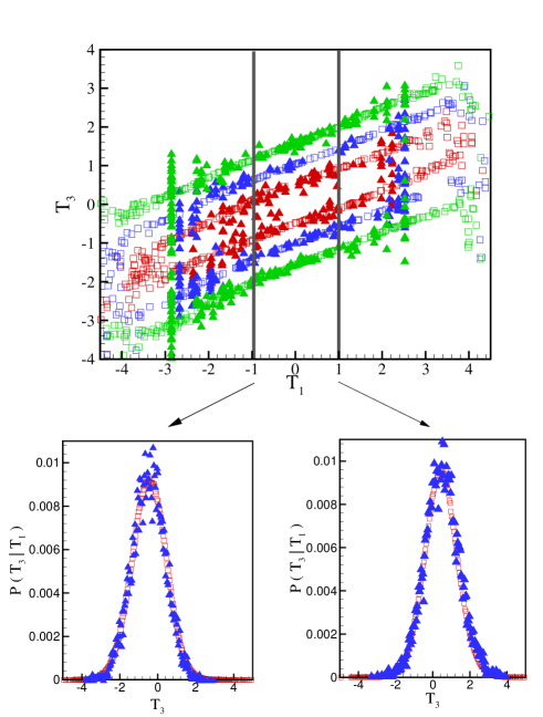
We checked the validity of the CK equation for describing the angular separation of $\hat{n}_{1}$ and $\hat{n}_{2}$ being equal to the Markov angular scale. This is shown in Fig. 5. In the upper panel we show the identification of the left (filled symbol) and right (open symbol) sides of Eq. (24) for three levels, 0.008 (red symbol), 0.005 (blue symbol), 0.002 (green symbol). The conditional PDF $P(T_{3}|T_{1})$, for $T_{1}=\pm\sigma$ are shown in the lower panel. All the scales are measured in unit of the standard deviation of the temperature fluctuations. The CK equation, formulated in differential form, yields the following Kramers-Moyal (KM) expansion [16],

$$\frac{\partial}{\partial\phi}P(T,\phi)=\sum_{n=1}^{\infty}(-\frac{\partial}{\partial T})^{n}[D^{(n)}(T,\phi)P(T,\phi)],$$ (25)

where $D^{(n)}(T,\phi)$ are called as the KM coefficients. These coefficients can be estimated directly from the moments $(M^{(n)})$ and the conditional probability distributions as:

$$D^{(n)}(T,\phi)=\frac{1}{n!}\hskip 5.69046pt\lim_{\Delta\phi\to 0}M^{(n)},$$ (26)

(27)

$$M^{(n)}=\frac{1}{\Delta\phi}\int dT^{\prime}(T^{\prime}-T)^{n}P(T^{\prime},\phi+\Delta\phi|T,\phi).$$ (28)

FIG. 5.: Verification of the validity of the Chapman-Kolmogorov equation (Eq. 24) for the angular separation of $\hat{n}_{1}$ and $\hat{n}_{2}$ being equal to the Markov angular scale. In the upper panel we show the identification of left (filled symbol) and right (open symbol) sides of Eq. (24) for three levels, 0.008 (red symbol), 0.005 (blue symbol), 0.002 (green symbol). The conditional PDFs $P(T_{3}|T_{1})$, for $T_{1}=\pm\sigma$ are shown at the lower panel. All the scales are measured in unit of the standard deviation of the temperature fluctuations.

FIG. 6.: The drift and diffusion coefficients, $D^{(1)}(T)$ and $D^{(2)}(T)$ in Eq. (28), following, respectively, linear and quadratic behaviors.

According to the Pawula’s theorem [16], for a process with $D^{(4)}\sim 0$, all the $D^{(n)}$ with $n\geq 3$ vanish, and the KM expansion reduces to the FP equation, known also as the Kolomogrov equation [16]

$$\frac{\partial}{\partial\phi}P(T,\phi)=\left[-\frac{\partial}{\partial T}D^{(1)}(T,\phi)+\frac{\partial^{2}}{\partial T^{2}}D^{(2)}(T,\phi)\right]P(T,\phi)\;.$$ (29)

Here $D^{(1)}(T,\phi)$ is the ’drift’ term, describing the deterministic part of the process, while $D^{(2)}(T,\phi)$ is the ‘diffusion’ term. Using the Ito interpretation, the FP equation is equivalent to the following Langevin equation [16]

$$\frac{d}{d\phi}T(\phi)=D^{(1)}(T)+\sqrt{D^{(2)}(T)}\hskip 2.84544ptf(\phi).$$ (30)

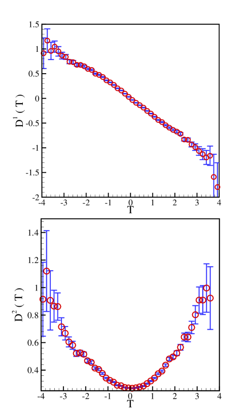
Here, $f(\phi)$ is a $\delta$-correlated Gaussian random force with zero mean (i.e., $<f(\phi)f(\phi^{\prime})>=3D\delta(\phi-\phi^{\prime})$). For the WMAP data, the drift and diffusion coefficients $D^{(1)}$ and $D^{(2)}$ are shown in Fig. 6. It turns out that the drift coefficient $D^{(1)}$ is a linear function in $T$, whereas the diffusion coefficient $D^{(2)}$ is a quadratic function. For large values of $T$, our estimates become poor and, thus, the uncertainty increases. From the analysis of the data set, we obtain the following approximate relations,

$$D^{(1)}(T)=-0.330T,$$ (31)

(32)

$$D^{(2)}(T)=0.060T^{2}+0.002T+0.270,$$ (33)

where we used the isotropy assumption which implies that $D^{(n)}(T,\phi)=D^{(n)}(T)$. The temperature field is measured in units of its standard deviation. The fourth-order coefficient $D^{(4)}$ is, in our analysis, ${D^{(4)}}\simeq 10^{-2}{D^{(2)}}$, so that we can ignore the coefficients $D^{(n)}$ for $n\geq 3$. Furthermore, using Eq. (30), it becomes clear that we are able to separate the deterministic and the noisy components of the CMB fluctuations in terms of the coefficients $D^{(1)}$ and $D^{(2)}$.

IV The (non)-Gaussianity test of CMB

Cosmological models of the structure formation are based on the standard inflationary paradigm, which implies Gaussian fluctuation of the density field [6, 7, 8, 18]. The Gaussianity in the density perturbation directly translates into the Gaussianity of the CMB temperature fluctuations. However, along with the standard inflationary models, there exist theories that predict the non-Gaussianity of the primordial fluctuations. Inflation with two or more scalar fields can provide significant deviations from the Gaussianity [19, 20, 21, 22]. Another possibility is the manipulation of the CMB data after the recombination, due to subsequent weak gravitational lensing [23, 24] and various foregrounds, such as dust emission, synchrotron radiation, or unresolved point sources [25]. One should also take into account the additional instrumental noise in the observational data [26].

There are standard methods of searching for non-Gaussian signature in the CMB data, such as using peak distributions [18, 27], the genus curve [28, 29], peak correlations [30] and global Minkowski functional methods [31]. More recent methods, such as a technique for studying hydrodynamic turbulence and detecting non-Gaussianity, and fractal analysis, can also be used for the CMB data [32, 33]. Moreover, the Gaussianity of the CMB at different angular scales have been tested [34, 35, 36, 37, 38, 39, 40, 41, 42, 43, 44, 45, 46, 47, 48, 49, 50, 51, 52, 53, 54, 55, 56, 57]. Most of the previous works were based on the consistency between the CMB data and simulated Gaussian realizations. So far, they have found no significant evidence for cosmological non-Gaussianity.

We note that for a Gaussian distribution, all the even moments are related to the second one through $\langle T^{2n}\rangle=\frac{2n!}{2^{n}n!}\langle T^{2}\rangle^{n}$ (e.g., for $n=2$, $\langle T^{4}\rangle=3\langle T^{2}\rangle^{2}$), while the odd moments are zero. We checked directly the relation between the moments for the CMB data. The results are summarized in Table I. The ratios $\langle T^{4}\rangle/(3\langle T^{2}\rangle^{2})$ are, $1.077\pm 0.004$ , $1.085\pm 0.005$ and $1.048\pm 0.005$, for the entire data set, and the northern and southern hemispheres, respectively. The odd moments $\langle T^{3}\rangle$ and $\langle T^{5}\rangle$ are not zero for different parts of the CMB data (see Table I). The odd moments of the temperature fluctuations can also be used as the indicators for the hot and cold spots. The southern part has a negative third moment, indicating greater prevalence of the cold spots, whereas the northern hemisphere has a positive third moment, indicating domination of the hot spots. The ratio of the higher moments, such as $\langle T^{6}\rangle/(15\langle T^{2}\rangle^{3})$, are, $1.398\pm 0.026$, $1.396\pm 0.022$ and $1.313\pm 0.035$ (for a Gaussian distribution this ration is unity) for the entire data set, and the northern and southern hemispheres, respectively.

The ratio of the higher moments, such as $\langle T^{6}\rangle/(15\langle T^{2}\rangle^{3})$, for the entire sky, and the northern and southern hemispheres are larger than those for a Gaussian distribution, implying that the probability distribution function for the temperature fluctuations in the CMB has fat tails compared to a Gaussian distribution.

Let us examine the predictions for the moments of the temperature fluctuations via the FP equation, and compare their values with the direct evaluation of results presented in Table I. Using the stochastic properties of the temperature field, one can check the deviation of the fluctuations from the Gaussian distribution in the northern and southern hemispheres, as well as in the entire data. As pointed out in section III, the PDF of the temperature fluctuations satisfies the KM expansion. Using Eq. (25) we calculate the $nth$ moment of the temperature fluctuations by multiplying both sides of Eq. (25) by $T^{n}$ and integrating over the temperature:

$$\frac{d}{d\phi}\langle T^{n}\rangle=\sum_{m=1}^{\infty}\frac{n!}{(n-m)!}\langle D^{(m)}(T)T^{n-m}\rangle.$$ (34)

We set $n=4$ in the above equation and find the equation for the fourth moment to be

$$\frac{d}{d\phi}\langle T^{4}\rangle=4\langle D^{(1)}(T)T^{3}\rangle+12\langle D^{(2)}(T)T^{2}\rangle$$ (35)

$$\qquad+24\langle D^{(3)}(T)T\rangle+24\langle D^{(4)}(T)\rangle.$$ (36)

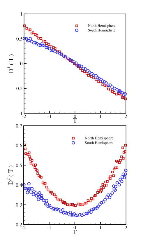
The KM coefficients for the northern and the southern hemispheres are given in Table II. For the isotropic case, all the moments of temperature fluctuations are independent of $\phi$, and the left-hand side of Eq. (35) vanishes. Using the results presented in Table II, for the northern and the southern hemispheres, Eq. (35) reduces to

$$\langle T^{4}\rangle_{north} = (2.71\pm 0.06)\langle T^{2}\rangle^{2}+(0.028\pm 0.010)\langle T^{3}\rangle\sqrt{\langle T^{2}\rangle},$$ (37)

$$\langle T^{4}\rangle_{south} = (3.27\pm 0.09)\langle T^{2}\rangle^{2}-(0.017\pm 0.020)\langle T^{3}\rangle\sqrt{\langle T^{2}\rangle},$$ (38)

where for the northern and southern hemispheres, $\langle T^{3}\rangle=(1.283\pm 0.125)\times 10^{-5}$, $\sqrt{\langle T^{2}\rangle}=(7.010\pm 0.004)\times 10^{-2}$ and $\langle T^{3}\rangle=(-5.408\pm 0.175)\times 10^{-5}$, $\sqrt{\langle T^{2}\rangle}=(7.914\pm 0.004)\times 10^{-2}$, respectively. We repeated the same procedure for the entire data set and obtained the following relation between the moments

$$\langle T^{4}\rangle=(3.07\pm 0.07)\langle T^{2}\rangle^{2}+(0.034\pm 0.020)\langle T^{3}\rangle\sqrt{\langle T^{2}\rangle},$$ (40)

where $\langle T^{3}\rangle=(-2.032\pm 0.108)\times 10^{-5}$ and $\sqrt{\langle T^{2}\rangle}=(7.475\pm 0.003)\times 10^{-2}$. The drift and diffusion coefficients of the northern and the southern hemisphere are shown in Fig. 7.

As mentioned earlier, for a Gaussian distribution, all the even moments are related to the second one, while the odd moments are zero. Eqs. (37) and (40) show that we have deviations from the Gaussianity, resulting from the coefficient of $\langle T^{2}\rangle^{2}$. Note that the result presented by Eq. (40) are compatible with direct calculation of moments for different part of the CMB data.

FIG. 7.: Drift and diffusion coefficients $D^{(1)}(T)$ and $D^{(2)}(T)$ for the northern and the southern hemisphere parts of the CMB data.

V Markov Nature of CMB and Angular Power Spectrum

Using statistical isotropy, the two-point temperature correlation function is expanded in term of the Legendre functions as

$$\langle T(\hat{n}_{1})T(\hat{n}_{2})\rangle=\sum_{l}\frac{2l+1}{4\pi}C_{l}P_{l}(\cos(\Theta)),$$ (41)

where $C_{l}$ is the angular power spectrum, $P_{l}$ is the Legendre polynomial of order $l$ and $\Theta=\arccos(\hat{n}_{1}.\hat{n}_{2})$. To find the relation between the Markovian properties of the CMB data and the $C_{l}$’s, we start with the temperature-increment moments, $S_{2}=\langle[T(\hat{n}_{1})-T(\hat{n}_{2})]^{2}\rangle$. The second moment $S_{2}$ allows us to determine $\langle T(\hat{n}_{1})T(\hat{n}_{2})\rangle$ and, hence, the $C_{l}$’s. On the other hand, $S_{2}$ can be obtained through $P(\Delta T,\Theta)$, where $\Delta T=T(\hat{n}_{1})-T(\hat{n}_{2})$. The FP equation [16] for $\Delta T(\Theta)$ is given by,

$$\frac{d}{d\Theta}P(\Delta T,\Theta)=$$ (42)

$$[-\frac{\partial}{\partial\Delta T}D^{(1)}(\Delta T,\Theta)+\frac{\partial^{2}}{\partial\Delta T^{2}}D^{(2)}(\Delta T,\Theta)]P(\Delta T,\Theta).$$ (43)

From the analysis of the CMB data we obtain the following equations for $D^{(1)}(\Delta T,\Theta)$ and $D^{(2)}(\Delta T,\Theta)$

$$D^{(1)}(\Delta T,\Theta)=(-0.190-\frac{0.182}{\Theta})\hskip 5.69046pt\Delta T,$$ (44)

(45)

$$D^{(2)}(\Delta T,\Theta)=[0.021+0.025\exp({-\frac{\Theta}{8.896}})](\Delta T)^{2}$$ (46)

$$\hskip 62.59596pt+0.279+\frac{0.014}{\Theta^{0.429}}.$$ (47)

Here, $\Delta T$ is measured in units of the standard deviation of $T$. Equation (42) allows us to obtain an equation for the second moment of the temperature increments, $S_{2}$. Multiplying Eq. (42) by $\Delta T^{2}$ and integrating over the increment of the temperature yield

$$\frac{d}{d\Theta}\langle T(\hat{n_{1}})T(\hat{n_{2}})\rangle=2[\alpha(\Theta)+\omega(\Theta)]\langle T(\hat{n_{1}})T(\hat{n_{2}})\rangle$$ (49)

$$\qquad-\sigma^{2}[2\alpha(\Theta)+2\omega(\Theta)-\beta(\Theta)],$$

where $\sigma^{2}=\langle T^{2}\rangle$, $D^{(1)}(\Delta T,\Theta)=\alpha(\Theta)\Delta T(\Theta)$, and $D^{(2)}(\Delta T,\Theta)=\beta(\Theta)\sigma^{2}+\lambda(\Theta)\sigma\Delta T(\Theta)+\omega(\Theta)\Delta T(\Theta)^{2}$. The coefficients $\alpha(\Theta)$, $\beta(\Theta)$, $\lambda(\Theta)$, and $\omega(\Theta)$ are given by Eq. (44).

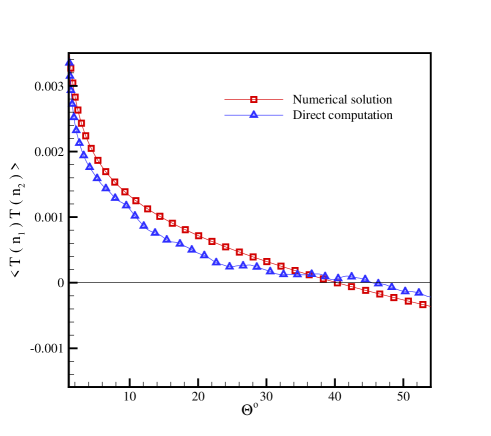
We obtain the correlation functions through numerical solution of Eq. (49) and compare it with the direct correlation shown in Fig. 8. The two approaches yield similar behavior. At $\Theta\simeq 39^{o}$ the correlation function vanishes. The relation between the KM coefficients with $C_{l}$ is then obtained by expanding the solution of Eq. (49) in terms of $P_{l}$.

FIG. 8.: Comparison of the numerical solution of Eq. (49) and direct computation of $\langle T(\hat{n_{1}})T(\hat{n_{2}})\rangle$.

VI Conclusion

We studied the stochastic nature of the temperature fluctuations in the CMB. The Markov angle, as the characteristic scale of the Markov properties of the CMB data, was obtained. According to the theory of stochastic process, the CMB data at scales larger than the Markov angle can be considered as a Markov process. This means that the data located at separations larger than the Markov scale can be described as a Markov chain. We also obtained the angular scale correlation for the CMB data and showed that it is independent of the Markov angular scale. This point can be explained as a simple example of the Brownian motion. Its dynamics is described by the Langevin equation, $\frac{dv}{dt}=-\alpha v+\eta(t)$ (similar to Eq. (30)), where the force $\eta(t)$ is a zero-mean Gaussian white noise. It is known that this process is a Markov process with a Markov time scale of unity [16]. On the other hand, the correlation time scale is of the order of $1/\alpha$, which is the characteristic time scale in the Langevin equation [16]. This means that for a Markovian process the Markov time scale does not depend on the correlation time scale.

We showed that the probability density of the temperature increments satisfies a Fokker-Planck equation that encodes the Markov property of the fluctuations. We gave the expressions for the Kramers-Moyal coefficients of the stochastic process $T$ and $\Delta T(\Theta)$, using the polynomial anzats [58, 59, 60, 61, 62, 63]. The Fokker-Planck equation enables us to derive a simple equation that governs the phenomenon in terms of azimuthal spherical coordinate. One of the important points that can be tested by this method is the (non)-Gaussianity of the temperature field.

Using the Fokker-Planck equation, we obtained the relation between the fourth and the lower moments, and observed small deviations from the Gaussianity. The same calculation was carried out by dividing the data into the northern and southern hemispheres. The PDF of the temperature exhibits fat tails for the northern and the southern hemispheres. The third moment indicates that, we have hot spots in the north, in contrast with the cold spots in the south hemisphere. To show a link between our method and the standard analysis of the CMB data through $C_{l}$ calculation, we obtained the evolution equation for the correlation function through the Fokker-Planck equation that governs the temperature increments. We found good agreement between our method and that of direct correlation function calculation.

The most important result of this paper is a possible interpretation of the CMB data in terms of the Markov angular scale. In this work we computed the Markov angular scale for the temperature fluctuations in the CMB, in the range of $1.01^{+0.09}_{-0.07}$, where comparison with the event horizon shows that the two angles are of the same order of magnitude. A possible interpretation may be the physical connection of the Markov angular scale for the CMB data to the event horizon at the last scattering surface.

From the definition of the event horizon, two points located further apart than the Markov angular scale do not connect gravitationally. From the inflationary scenario for the early universe, all the points in the universe have been correlated during the inflationary epoch, and get almost uniform Harrison-Zel’dovich spectrum. After the end of the inflation, the perturbation remained from the inflation started to grow and the gravitational effect of each point could travel within the event horizon scales, so that outside the horizon we have the primordial spectrum from the inflation, while inside the horizon this spectrum has been vanished due to the gravitational interaction between the points. The result is that, if we look at the density perturbation in the CMB as a stochastic field, the conditional probability of finding two points inside the event horizon scale will depend on all the particles in between, while for the points outside the event horizon, the memory of scale-invariant spectrum should be restored. A better interpretation of this issue needs a $N$-body simulation of structure formation from the inflationary epoch to the last scattering surface, together with a simultaneous calculation of the Markov length.

We would like to acknowledge the WMAP team for providing us with their data. We thank R. Ansari, H. Arfaei, V. Karimipour, R. Mansouri, N. Taghavinia, M. A. Vesaghi and M. Sahimi for useful discussions. This work was supported by the Research Institute for Astronomy and Astrophysics of Maragha-Iran.

TABLE I.: The values of Moments $\langle T^{n}\rangle$ for whole sphere, northern and the southern hemisphere of the CMB map data.

	$\langle T^{2}\rangle$	$\langle T^{3}\rangle$	$\langle T^{4}\rangle$	$\langle T^{5}\rangle$
Whole-sphere	$(5.588\pm 0.005)\times 10^{-3}$	$(-2.033\pm 0.108)\times 10^{-5}$	$(1.009\pm 0.003)\times 10^{-4}$	$(-1.298\pm 0.132)\times 10^{-6}$
Northern-hemisphere	$(4.914\pm 0.006)\times 10^{-3}$	$(1.283\pm 0.125)\times 10^{-5}$	$(7.867\pm 0.0305)\times 10^{-5}$	$(7.632\pm 1.028)\times 10^{-7}$
Southern-hemisphere	$(6.264\pm 0.007)\times 10^{-3}$	$(-5.408\pm 0.175)\times 10^{-5}$	$(1.233\pm 0.005)\times 10^{-4}$	$(-3.392\pm 0.244)\times 10^{-6}$

TABLE II.: The values of Kramers-Moyal coefficients for the northern and the southern hemisphere of the CMB map data.

	$D^{(1)}(T)$	$D^{(2)}(T)$	$D^{(3)}(T)$	$D^{(4)}(T)$
Northern-hemisphere	-0.370$T$	0.290-0.003$T$+0.075$T^{2}$	-0.001-0.110$T$	0.040-0.007$T$+0.0182$T^{2}$
			+0.003$T^{2}$-0.010$T^{3}$	-0.0005$T^{3}$+0.001$T^{4}$
Southern-hemisphere	-0.290$T$	0.250+0.007$T$+0.047$T^{2}$	0.004-0.078$T$	0.031-0.003$T$+0.020$T^{2}$
			-0.005$T^{2}$-0.003$T^{3}$	+0.001$T^{3}$-0.001$T^{4}$

REFERENCES

- [1] N. Afshordi, Y. Loh, M. A. Strauss, Phys. Rev. D, 69, 083524 (2004).
- [2] C. L. Bennett, et al., ApJS, 148, 213 (2003).
- [3] D. N. Spergel, et al., ApJS, 148, 175 (2003).
- [4] M. Tegmark, et al., Phys. Rev. D 69, 103501 (2004).
- [5] H. V. Peiris, et al., ApJS 148, 213 (2003).
- [6] V. F. Mukhanov and G. Chbisov, JETP Letters 33, 532 (1981).
- [7] S. W. Hawking, Phys. Lett. B 115, 295 (1982).
- [8] A. H. Guth and S. Y. Pi, Phys. Rev. Lett. 49, 1110 (1985).
- [9] C. L. Bennett et al. ApJ 581, 1 (2003).
- [10] L. Page et al. ApJS 148, 39 (2003).
- [11] Peebles, P. J., ”The Large Scale Structure of the Universe” Princeton University press, 1980.
- [12] E. P. Donoghue, J. F. Donoghue, Phys. Rev. D 71, 043002 (2005); A. Hajian, T. Souradeep and N. Cornish, ApJ, 618, 63 (2004); S. Movahed, F. Ghasemi, S. Rahvar and M. R . Rahimi Tabar, submitted to Phys. Rev D (arXive:astro-ph/0602461).
- [13] Friedrich, R., Zeller J., and Peinke J., 1998, Europhys. Lett. 41, 153.
- [14] Jafari, G. R., Fazlei, S. M., Ghasemi, F., Vaez Allaei, S. M., Rahimi Tabar, M. R., Iraji Zad A. and Kavei, G., 2003, Phys. Rev. Lett. 91 226101.
- [15] F. Ghasemi, Peinke J., Sahimi M. and Reza Rahimi Tabar M., Eur. Phys. J. B 47, 411?415 (2005)
- [16] Risken H. ”The Fokker-Planck equation” Springer, Berlin, 1984.
- [17] Jr. R.Colistete , J.C. Fabris, S. V. B. Goņcalves and P. E. de Souza , Int. J. Mod. Phys. D 13, 669 (2004).
- [18] Bardeen, J. M., Bond, J. R., Kaiser, N., and Szalay, A. S., 1986, Ap. J. 304,15.
- [19] A. Linde and V. F. Mukhanov, Phys. Rev. D 56, 535 (1997). Nongaussian Isocurvature Perturbations from Inflation’, astro-ph/9705200.
- [20] P. J. E. Peebles, Ap.J. 510, 531 (1999).
- [21] P. J. E. Peebles, Ap.J. 510, 523 (1999).
- [22] Antoniadis, I., Mazur, P. O., and Mottola, E., 1997, Comment on ” Nongaussian Isocurvature Perturbations from Inflation’, astro-ph/9705200.
- [23] T. Fukushige, J. Makino, O. Nishimura and T. Ebisuzaki, Publications of the Astronomical Society of Japan 47, 493 (1995).
- [24] Bernardeau, F., 1997, Astron. Astrophys. 324, 15.
- [25] Banday, A. J., GórskiK. M., Bennett, C. L., Hinshaw, G., Kogut, A., and Smoot, G. F., 1996, Ap. J. 468, L85.
- [26] Tegmark, M., 1997, Ap. J. 480, L87.
- [27] J. R. Bond, and G. Efstathiou, Mon. Not. Roy. Astron. Soc. 226, 655 (1987).
- [28] P. Coles, Mon. Not. Roy. Astron. Soc. 234, 509 (1988).
- [29] G. F. Smoot, L. Tenorio, A. Kogut, E. L. Wright, Ap. J. 437, 1 (1994).
- [30] A. Kogut, A. J. Banday, Ap. J. Lett. 464, L29 (1996).
- [31] S. Winitzki, and A. Kosowsky, New Astronomy 3, 75 (1997).
- [32] A. Bershadskii and K. R. Sreenivasan, Phys. Lett. A. 319, 21 (2003).
- [33] S. Movahed et. al., arXive:astro-ph/0602461.
- [34] A. F. Heavens, Mon. Not. Roy. Astron. Soc. 299, 805 (1998).
- [35] J. Schmalzing and K.M. Gorski, Mon. Not. Roy. Astron. Soc. 297, 355 (1998).
- [36] P. G. Ferreira, J. Magueijo and K. M. Górski, Ap. J. Lett. 503, L1 (1998).
- [37] J. Pando, D. Valls-Gabaud and L. Z. Fang, Phys. Rev. Lett. 81, 4568 (1998).
- [38] B. C. Bromley and M. Tegmark, Ap. J. Lett. 524, L79 (1999).
- [39] A. J. Banday, S. Zaroubi and K. M. Górski, Ap. J. 533, 575 (2000).
- [40] C. R. Contaldi, P. G. Ferreira, J. Magueijo and K. M. Górski, Ap. J. 534, 25 (2000).
- [41] P. Mukherjee, M. P. Hobson and A. N. Lasenby, Mon. Not. Roy. Astron. Soc. 318, 1157 (2000).
- [42] J. Magueijo, Ap. J. Lett. 528, L57 (2000).
- [43] D. Novikov, J. Schmalzing and V. F. Mukhanov, A&A 364, 17 (2000).
- [44] H. B. Sandvik and J. Magueijo, Mon. Not. Roy. Astron. Soc. 325, 463 (2001).
- [45] J. Magueijo, Ap. J. Lett. 528, L57 (2000).
- [46] R. B. Barreiro, M. P. Hobson, A. N. Lasenby, A. J. Banday, K. M. Górski and G. Hinshaw, Mon. Not. Roy. Astron. Soc. 318, 475 (2000).
- [47] N. G. Phillips and A. Kogut, Ap. J. 548, 540 (2001).
- [48] E. Komatsu and U. Seljak, Mon. Not. Roy. Astron. Soc. 336, 1256 (2002).
- [49] E. Komatsu and D. N. Spergel, Phys. Rev. D 63, 63002 (2001).
- [50] M. Kunz, A. J. Banday, P. G. Castro, P. G. Ferreira and K. M. Górski, Ap. J. Lett. 563, L99 (2001).
- [51] N. Aghanim, O. Forni and F. R. Bouchet, A&A 365, 341 (2001).
- [52] L. Cayón, E. Martinez-Gonzalez, F. Argueso, A. J. Banday and K. M. Górski, Mon. Not. Roy. Astron. Soc., 339, 1189 (2003).
- [53] C. Park, B. Ratra and M. Tegmark, Ap. J. 556, 582 (2001).
- [54] S. F. Shandarin, H. A. Feldman, Y. Xu and M. Tegmark, Ap. J. S. 141, 1 (2002).
- [55] J. H. Wu et al., Phys. Rev. Lett. 87, 251303 (2001).
- [56] M. G. Santos, A. Cooray, Z. Haiman, L. Knox and Ch. Ma., Ap. J. 598, 756 (2003).
- [57] G. Polenta et al., Ap. J. Lett. 572, L27 (2002).
- [58] Friedrich, R., Peinke, J., 1997, Phys. Rev. Lett. 78, 863.
- [59] Friedrich, R., Peinke, J. and Renner, C., 2000, Phys. Rev. Lett, 84, 5224.
- [60] Friedrich R., Marzinzik k. & Schmigel A., in ”A perspective Look at Nonlinear Media”, Edited by Jurgen Parisi, Stefan C. Muller and Walter Zimmermann, Lecture notes in Physics, Vol. 503, P. 313 (Springer-verlag, Berlin, 1997)
- [61] Davoudi, J., Rahimi Tabar, R. M., 1999, Phys. Rev. Lett. 82, 1680.
- [62] Ragwitz M., Kantz H., 2001, Phys. Rev. Lett. 87, 254501.
- [63] Friedrich R., Renner C., Siefert M. and Peinke J., 2002, Phys. Rev. Lett. 89, 149401.