Constraints on braneworld inflation from CMB anisotropies

Abstract

We obtain observational constraints on Randall–Sundrum type II braneworld inflation using a compilation of data including WMAP, the 2dF and latest SDSS galaxy redshift surveys. We place constraints on three classes of inflation models (large-field, small-field and hybrid models) in the high-energy regime, which exhibit different behaviour compared to the low-energy case. The quartic potential is outside the $2\sigma$ observational contour bound for a number of $e$-folds less than 60, and steep inflation driven by an exponential potential is excluded because of its high tensor-to-scalar ratio. It is more difficult to strongly constrain small-field and hybrid models due to additional freedoms associated with the potentials, but we obtain upper bounds for the energy scale of inflation and the model parameters in certain cases. We also discuss possible ways to break the degeneracy of consistency relations and inflationary observables.

I Introduction

The recent publication of data from the Wilkinson Microwave Anisotropy Probe (WMAP) Spergel:2003cb has brought the global cosmological dataset to a precision where it seriously constrains inflationary models Peiris:2003ff ; Barger:2003ym ; Bridle ; Kinney:2003uw ; Leach:2003us ; Tegmark . The observations show strong support for the standard inflationary predictions of a flat Universe with adiabatic density perturbations, and in particular, the viable parameter space of slow-roll inflation models in the standard cosmology has been significantly narrowed. We are now entering a golden age where the physics in the early universe can be probed by upcoming high-precision observational data.

It is now possible also to impose observational constraints on inflation in non-standard cosmologies, the archetypal example being the braneworld cosmology, and in particular the Randall–Sundrum Type II model (RSII) RSII which is the one most investigated in the literature. While it has been shown that observations of the primordial spectra cannot distinguish between the standard cosmology and the braneworld Liddle01 , specific constraints on the potential driving inflation will be different between those scenarios. Liddle and Smith Liddle:2003gw recently imposed the first constraints on such models, studying the case of monomial potentials $V\propto\phi^{p}$ in the RSII braneworld and finding that the constraints on $p$ tighten in the braneworld regime.

In this paper we aim to make a much more general analysis of constraints on inflationary models in the RSII braneworld, under the assumption that inflation takes place in the high-energy regime of such theories. We will use the current observational datasets, including the latest Sloan Digital Sky Survey (SDSS) power spectrum data SDSS , and seek to impose constraints for a range of different types of inflationary model.

II Formalism

In the RSII model RSII , where matter fields are confined to the brane, the Einstein equations can written as SMS :

$${}^{(4)}G_{\mu\nu}=-\Lambda_{4}g_{\mu\nu}+\frac{8\pi}{m_{{\rm Pl}}^{2}}T_{\mu\nu}+\left(\frac{8\pi}{M_{5}^{3}}\right)^{2}\pi_{\mu\nu}-E_{\mu\nu},$$ (1)

where $T_{\mu\nu}$ and $\pi_{\mu\nu}$ represent the energy–momentum tensor on the brane and a quadratic term in $T_{\mu\nu}$, respectively. $E_{\mu\nu}$ is a part of the 5-dimensional Weyl tensor, which carries the information about the bulk. The 4- and 5-dimensional Planck scales, $m_{{\rm Pl}}$ and $M_{5}$, are related via the 3-brane tension, $\lambda$, as

$$\lambda=\frac{3}{4\pi}\frac{M_{5}^{6}}{m_{{\rm Pl}}^{2}}\,.$$ (2)

Hereafter the 4-dimensional cosmological constant $\Lambda_{4}$ is assumed to be zero.

Adopting a flat Friedmann–Robertson–Walker (FRW) metric as a background spacetime on the brane, the Friedmann equation becomes

$$H^{2}\equiv\left(\frac{\dot{a}}{a}\right)^{2}=\frac{8\pi}{3m_{{\rm Pl}}^{2}}\rho\left(1+\frac{\rho}{2\lambda}\right)\,,$$ (3)

where $a$, $H$, and $\rho$ are the scale factor, the Hubble parameter, and the energy density of the matter on the brane, respectively. We ignored the so-called ‘dark radiation’, $E_{\mu\nu}$, which decreases as $\sim a^{-4}$ during inflation (we caution that this can be important in considering perturbations at later stages of cosmological evolution Koyama:2003be ). At high energies the $\rho^{2}$ term is expected to play an important role in determining the evolution of the Universe.

The inflaton field $\phi$, confined to the brane, satisfies the Klein–Gordon equation

$$\ddot{\phi}+3H\dot{\phi}+V^{\prime}(\phi)=0\,,$$ (4)

where $V(\phi)$ is the inflaton potential and a prime denotes a derivative with respect to $\phi$. The quadratic contribution in Eq. (3) increases the Hubble expansion rate during inflation, which makes the evolution of the inflaton slower through Eq. (4). Combining Eq. (3) with Eq. (4), we get the following equation Maartens:1999hf ; Tsujikawa:2000hi

$$\frac{\ddot{a}}{a}=\frac{8\pi}{3m_{{\rm Pl}}^{2}}\left[(V-\dot{\phi}^{2})+\frac{\dot{\phi}^{2}+2V}{8\lambda}(2V-5\dot{\phi}^{2})\right]\,.$$ (5)

The condition for inflation is $\ddot{a}>0$, which reduces to the standard expression $V>\dot{\phi}^{2}$ for $(\dot{\phi}^{2}+2V)/8\lambda\ll 1$. In the high-energy case, this condition corresponds to $2V>5\dot{\phi}^{2}$, which means that inflation ends around $2V\simeq 5\dot{\phi}_{f}^{2}$. Making use of the slow-roll conditions in Eqs. (3) and (4), the end of inflation is characterized by

$$\frac{V^{3}(\phi_{f})}{V^{\prime 2}(\phi_{f})}\simeq\frac{5\lambda m_{{\rm Pl}}^{2}}{24\pi}\,.$$ (6)

The amplitudes of scalar and tensor perturbations generated in RSII inflation are given as Maartens:1999hf ; Langlois2

$$A_{{\rm S}}^{2} = \frac{512\pi}{75m_{{\rm Pl}}^{6}}\,\frac{V^{3}}{V^{\prime 2}}\,\left(1+\frac{V}{2\lambda}\right)^{3}\Biggr{|}_{k=aH}\,,$$ (7)

$$A_{{\rm T}}^{2} = \frac{4}{25\pi}\,\frac{H^{2}}{m_{{\rm Pl}}^{2}}\,F^{2}(x)\Biggr{|}_{k=aH}\,,$$ (8)

where $x=Hm_{{\rm Pl}}\sqrt{3/(4\pi\lambda)}$ and

$$F(x)=\left[\sqrt{1+x^{2}}-x^{2}\sinh^{-1}(1/x)\right]^{-1/2}\,.$$ (9)

The right hand sides of Eqs. (7) and (8) are evaluated at Hubble radius crossing, $k=aH$ (here $k$ is the comoving wavenumber).

Defining the spectral indices of scalar and tensor perturbations as

$$n_{{\rm S}}-1\equiv\frac{{\rm d}\ln A_{{\rm S}}^{2}}{{\rm d}\ln k}\Biggr{|}_{k=aH}\,,~{}~{}~{}n_{{\rm T}}\equiv\frac{{\rm d}\ln A_{{\rm T}}^{2}}{{\rm d}\ln k}\Biggr{|}_{k=aH}\,,$$ (10)

and making use of the slow-roll conditions in Eqs. (3) and (4), one finds Maartens:1999hf ; Huey:2001ae

$$n_{{\rm S}}-1=-6\epsilon+2\eta\quad,\quad n_{{\rm T}}=-\frac{2}{N^{\prime}}\frac{x^{\prime}}{x}\frac{F^{2}}{\sqrt{1+x^{2}}}\,.$$ (11)

where $\epsilon$ and $\eta$ are slow-roll parameters, defined by

$$\epsilon \equiv \frac{m_{{\rm Pl}}^{2}}{16\pi}\,\left(\frac{V^{\prime}}{V}\right)^{2}\;\frac{1+V/\lambda}{\left(1+V/2\lambda\right)^{2}}\,,$$ (12)

$$\eta \equiv \frac{m_{{\rm Pl}}^{2}}{8\pi}\,\frac{V^{\prime\prime}}{V}\;\frac{1}{1+V/2\lambda}\,,$$ (13)

together with the number of $e$-folds

$$N\simeq-\frac{8\pi}{m_{{\rm Pl}}^{2}}\int^{\phi_{f}}_{\phi}\frac{V}{V^{\prime}}\left(1+\frac{V}{2\lambda}\right)d\phi\,.$$ (14)

Here $\phi_{f}$ is the value of the inflaton at the end of inflation.

We shall define the ratio of tensor to scalar perturbations as

$$R\equiv 16\,\frac{A_{{\rm T}}^{2}}{A_{{\rm S}}^{2}}\,,$$ (15)

which coincides with the definition of $R$ in Refs. Peiris:2003ff ; Barger:2003ym ; Tegmark $R\simeq 16\epsilon$, in the low-energy limit. From Eqs. (7), (8), (11) and (15), one can show that the following consistency relation holds independent of the brane tension, $\lambda$, as Huey:2001ae

$$n_{\rm T}=-R/8\,.$$ (16)

That the consistency equation is unchanged in the RSII braneworld means that the perturbations do not contain any extra information as compared to the standard cosmology. In particular, this means that they cannot be used to determine the brane tension $\lambda$; for any value of $\lambda$ a potential can always be found to generate any observed spectra Liddle01 . This result has a nice expression in terms of the horizon-flow parameters defined by STG ; Sam

$$\epsilon_{0}=\frac{H_{\rm inf}}{H}\,,~{}~{}~{}\epsilon_{i+1}=\frac{{\rm dln}|\epsilon_{i}|}{{\rm d}N}\,,~{}~{}~{}(i\geq 0)\,,$$ (17)

where $H_{\rm inf}$ is the Hubble rate at some chosen time. Then we have

$$n_{{\rm S}} = 1-2\epsilon_{1}-\epsilon_{2},~{}n_{{\rm T}}=-2\epsilon_{1},~{}R=16\epsilon_{1}\,,$$ (18)

$$\alpha_{{\rm S}} = -2\epsilon_{1}\epsilon_{2}-\epsilon_{2}\epsilon_{3}\,,~{}\alpha_{\rm T}=-2\epsilon_{1}\epsilon_{2}\quad({\rm for}~{}~{}V/\lambda\ll 1)$$

and

$$n_{{\rm S}} = 1-3\epsilon_{1}-\epsilon_{2},~{}n_{{\rm T}}=-3\epsilon_{1},~{}R=24\epsilon_{1}\,,$$ (19)

$$\alpha_{{\rm S}} = -3\epsilon_{1}\epsilon_{2}-\epsilon_{2}\epsilon_{3}\,,~{}\alpha_{\rm T}=-3\epsilon_{1}\epsilon_{2}\quad({\rm for}~{}~{}V/\lambda\gg 1)$$

where $\alpha_{{\rm S},{\rm T}}\equiv dn_{{\rm S},{\rm T}}/d\ln k$ are the runnings of the two spectra. We see that these two sets of expressions become identical if one associates $2\epsilon_{1}$ in the low-energy limit with $3\epsilon_{1}$ in the high-energy limit.

The upshot of this correspondence is that a separate likelihood analysis of observational data is not needed for the braneworld scenario, as observations can be used to constrain the same parametrization of the spectra produced. However, when those constraints are then interpreted in terms on the form of the inflationary potential, differences will be seen depending on the regime we are in. For the remainder of this paper, we will obtain constraints under the assumption that we are in the high-energy regime. Our work extends that of Liddle and Smith Liddle:2003gw who examined only monomial potentials, though they did so for a general $\lambda$.

III Likelihood analysis

In order to compare the theoretical predictions of braneworld inflation with observed CMB anisotropies, we run the CAMB program developed in Ref. antony1 coupled to the CosmoMc (Cosmological Monte Carlo) code antony2 . This code makes use of a Markov-chain Monte Carlo method to derive the likelihood values of model parameters. In addition to the data sets from WMAP WMAP , we include the band-powers on smaller scales corresponding to $800<l<2000$, from the VSA VSA , CBI CBI , ACBAR ACBAR , and the 2dF 2dF and latest SDSS galaxy redshift surveys SDSS . We include both 2dF and SDSS under the assumption that they can be treated as statistically independent, but in fact little difference arises if either one is dropped. The CosmoMc code generates a large set of power spectra for given values of cosmological and inflationary model parameters, and finds the likelihood values of parameters by comparing the temperature (TT) and temperature–polarization cross-correlation (TE) anisotropy spectra and the matter power spectrum with recent data.

The WMAP team Peiris:2003ff carried out the likelihood analysis by varying the four quantities $A_{\rm S}$, $R$, $n_{\rm S}$ and $\alpha_{\rm S}$. The quantities $n_{\rm T}$ and $\alpha_{\rm T}$ are related to those by consistency equations, and $\alpha_{\rm T}$ has anyway always been ignored so far in parameter fits as its cosmological consequences are too subtle for current or near-future data to detect.

In adopting an expansion of the spectra, one should be careful about convergence criteria. The power spectrum $A_{\rm S}^{2}(k)$ is generally expanded in the form Lidsey:1995np

$${\rm ln}\,A_{\rm S}^{2}(k) = {\rm ln}\,A_{\rm S}^{2}(k_{*})+(n_{\rm S}-1)\,{\rm ln}\left(\frac{k}{k_{*}}\right)$$ (20)

$$+\frac{\alpha_{\rm S}}{2}\,{\rm ln}^{2}\left(\frac{k}{k_{*}}\right)+\cdots\,,$$

where $k_{*}$ is some pivot wavenumber. In order for this Taylor expansion to be valid, we require the following condition Leach:2003us

$$|n_{\rm S}-1|\gg\left|\frac{\alpha_{\rm S}}{2}{\rm ln}\left(\frac{k}{k_{*}}\right)\right|\,.$$ (21)

For the maximum values $|{\rm ln}\left(k/k_{*}\right)|\sim 10^{4}$ and $|n_{\rm S}-1|\lesssim 0.07$, one gets the convergence criterion $|\alpha_{\rm S}|\lesssim 0.03$. If this condition is not imposed, the likelihood results are not expected to be completely reliable. We numerically found that the ratio $R$ shifts toward larger likelihood values if the upper bound of $\alpha_{\rm S}$ is chosen to be greater than 0.03. This implies that it is important to choose an appropriate prior for $\alpha_{\rm S}$ in order to get a good convergence for inflationary model parameters.

When one performs a likelihood analysis using horizon-flow parameters, the $2\sigma$ upper limits of $\epsilon_{1}$ and $\epsilon_{2}$ were found to be $0<\epsilon_{1}<0.032$ and $-0.15<\epsilon_{2}<0.08$ in the low-energy limit ($V/\lambda\to 0$) Leach:2003us . Since $\epsilon_{3}$ is poorly constrained and is consistent with zero, it could be set to zero and then the running ranges $-0.0096<\alpha_{\rm S}<0.0051$ from Eq. (II), which is well inside the convergence criterion.

The high-energy case ($V/\lambda\to\infty$) corresponds to changing the above $\epsilon_{1}$ to $(3/2)\epsilon_{1}$. Since $n_{\rm T}$, $\alpha_{\rm S}$ and $\alpha_{\rm T}$ are written in terms of $n_{\rm S}$, $R$ and $\epsilon_{3}$, from Eqs. (16) and (19), we perform the likelihood analysis by varying four quantities: $n_{\rm S}$, $R$, $\epsilon_{3}$ and $A_{\rm S}^{2}$. This is equivalent to varying three horizon-flow parameters ($\epsilon_{1},\epsilon_{2},\epsilon_{3}$) in Eq. (19) in addition to $A_{\rm S}^{2}$. We put a prior $0.8<n_{\rm S}<1.15$ and $0<R<0.7$, in which case the convergence criterion, $|\alpha_{\rm S}|\lesssim 0.03$, is satisfied. We found that $\epsilon_{3}$ is poorly constrained as pointed out in Ref. Leach:2003us , which means that the present observation does not reach the level to constrain the higher-order slow-roll parameters. Two dimensional observational constraints in terms of $n_{\rm S}$ and $R$ are plotted in Fig. 1. The allowed range of inflationary parameters is tighter than the results by Barger et al. Barger:2003ym , since we implement several independent cosmological parameters in addition to WMAP measurement. Our results are consistent with the recent work by the SDSS group Tegmark .

We varied 4 cosmological parameters ($\Omega_{b}h^{2}$, $\Omega_{c}h^{2}$, $Z=e^{-2\tau}$, $H_{0}$) as well in addition to 4 inflationary variables by assuming a flat $\Lambda$CDM universe. Here $\Omega_{b}h^{2}$ and $\Omega_{c}h^{2}$ are the baryon and dark matter density, $\tau$ is the optical depth, and $H_{0}$ is the Hubble constant. As seen in Fig. 2, the likelihood values of these basic cosmological parameters agree well with past works Peiris:2003ff ; Barger:2003ym ; Bridle ; Kinney:2003uw ; Leach:2003us ; Tegmark .

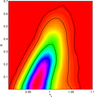
Figure 1: 2D posterior constraints in the $n_{\rm S}$-$R$ plane. We also show the $1\sigma$, $2\sigma$ and $3\sigma$ contour bounds. The region with a light colour corresponds to the likelihood region. The ratio $R$ is constrained to be $R<0.57$ at the $2\sigma$ level.

Figure 2: Marginalized probability distributions of the cosmological & inflationary parameters. We find that the distribution is well described by a Gaussian.

IV Constraints on braneworld inflation

In this section we shall consider constraints on single-field braneworld inflation in the high-energy case ($V/\lambda\gg 1$). We can classify models of inflation in the following way Kolb . The first class (type I) is the “large-field” model, in which the initial value of the inflaton is large and it rolls down toward the potential minimum at smaller $\phi$. Chaotic inflation Linde83 is one of the representative models of this class. The second class (type II) is the “small-field” model, in which the inflaton field is small initially and slowly evolves toward the potential minimum at larger $\phi$. New inflation Newinf and natural inflation Natural are the examples of this type. The third one (type III) is the hybrid (double) inflation model hybrid ; hybrid2 , in which inflation ends by a phase transition triggered by the presence of the second scalar field (or after a second phase of inflation following the phase transition).

When $V/\lambda\gg 1$ we have

$$n_{\rm S}-1 = -\frac{m_{{\rm Pl}}^{2}}{2\pi}\frac{\lambda}{V}\left[3\left(\frac{V^{\prime}}{V}\right)^{2}-\frac{V^{\prime\prime}}{V}\right]\,,$$ (22)

$$R = \frac{6m_{{\rm Pl}}^{2}}{\pi}\left(\frac{V^{\prime}}{V}\right)^{2}\frac{\lambda}{V}\,.$$ (23)

In this case the relation between $n_{\rm S}$ and $R$ can be written as

$$R=4(1-n_{\rm S})+8\eta\,.$$ (24)

The border of large-field and small-field models is given by the linear potential

$$V=m\phi\,.$$ (25)

Since $V^{\prime\prime}$ vanishes in this case (i.e., $\eta=0$), the spectral index of scalar perturbations is $n_{\rm S}-1=-6\epsilon$ from Eq. (11). In this case we have

$$R=4(1-n_{\rm S})\,.$$ (26)

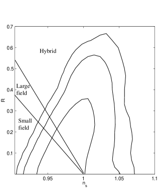
Figure 3: Classification of inflationary models in the $n_{\rm S}$-$R$ plane in the high energy limit. The line $R=4(1-n_{\rm S})$ marks the border of large- and small-field models, whereas the border of large-field and hybrid models corresponds to $R=6(1-n_{\rm S})$.

The exponential potential

$$V=V_{0}\exp\left(-\sqrt{\frac{16\pi}{\alpha}}\frac{\phi}{m_{{\rm Pl}}}\right)\,,$$ (27)

characterizes the border of large-field and hybrid models. In the high-energy limit, we have $\epsilon=\eta=4\lambda/(V\alpha)$, $n_{\rm S}-1=-16\lambda/(V\alpha)$ and $R=96\lambda/(V\alpha)$, thereby yielding

$$R = 6(1-n_{\rm S})\,.$$ (28)

In Fig. 3 we plot the borders (26) and (28) together with the regions of three kinds of inflationary models. The allowed range of hybrid models is wide relative to large-field and small-field models.

IV.1 Large-field models

Large-field models correspond to the parameter range with $0<\eta\leq\epsilon$. The inflaton potential in these models is characterized as

$$V(\phi)=c\phi^{p}\,.$$ (29)

For a fixed value of $p$ we have one free parameter, $c$, associated with the potential.

From Eqs. (22) and (23) one gets

$$n_{\rm S}-1 = -\frac{\lambda m_{{\rm Pl}}^{2}p(2p+1)}{2\pi c\phi^{p+2}}\,,$$ (30)

$$R = \frac{6\lambda m_{{\rm Pl}}^{2}p^{2}}{\pi c\phi^{p+2}}\,,$$ (31)

which means that $n_{\rm S}$ and $R$ are the functions of $\lambda$, $c$ and $\phi$. From Eq. (6) we find that inflation ends at

$$\phi_{f}^{p+2}=\frac{5p^{2}M_{5}^{6}}{32\pi^{2}c}\,,$$ (32)

where we used the relation Eq. (2). The number of $e$-folds is

$$N=\frac{4\pi c}{\lambda m_{{\rm Pl}}^{2}p(p+2)}\phi^{p+2}-\frac{5p}{6(p+2)}\,.$$ (33)

The second term ranges $5/12<p<5/6$ for $p>2$, thus negligible for $N\gtrsim 50$. Then we have the following relation

$$n_{\rm S}-1 = -\frac{2(2p+1)}{N(p+2)}\,,$$ (34)

$$R = \frac{24p}{N(p+2)}\,.$$ (35)

This is slightly different from what was obtained in Ref. Liddle:2003gw as we neglected the contribution coming from the second term in Eq. (33). For a fixed value of $p$, $n_{\rm S}$ and $R$ are only dependent on $N$.

From Eqs. (34) and (35) we get

$$R=\frac{12p}{2p+1}(1-n_{\rm S})\,,$$ (36)

which corresponds to a straight line for a fixed $p$. For larger $p$, the tangent of the line Eq. (36) gets larger. In Fig. 4 we plot the values of $n_{\rm S}$ and $R$ for different values of $N$ and $p$. Note that we consider several values of $e$-foldings which range $45\leq N\leq 60$, whereas in Ref. Liddle:2003gw this is fixed to be $N=55$.

When $p=2$ the theoretical predictions Eqs. (34) and (35) are within the $2\sigma$ observational contour bound for $N>50$ as found from Fig. 4. On the other hand the quartic potential ($p=4$) is under strong observational pressure; the model is outside the $2\sigma$ bound for $N\lesssim 60$. This case is disfavoured observationally, as in the case of standard inflation Peiris:2003ff ; Barger:2003ym ; Bridle ; Kinney:2003uw ; Leach:2003us ; Tegmark .

The exponential potential Eq. (27) corresponds to the limit $p\to\infty$, in which case we have $n_{\rm S}-1=-4/N$ and $R=24/N$ from Eqs. (34) and (35). This case does not lie within the $2\sigma$ bound unless $N\gtrsim 90$. Therefore the steep inflation Copeland:2000hn driven by an exponential potential is excluded observationally. Although inflation is realized even for $\alpha<1$ in Eq. (27) in braneworld, the spectral index $n_{\rm S}$ and the ratio $R$ are shifted from the point $n_{\rm S}=1$ and $R=0$ due to the steepness of the potential.

For the potential Eq. (29) the amplitude of scalar perturbations is given as

$$A_{{\rm S}} \simeq \frac{64\pi^{2}c^{2}}{45pM_{5}^{9}}\phi^{2p+1}\,$$ (37)

$$\simeq \frac{64\pi^{2}c^{2}}{45pM_{5}^{9}}\left(\frac{3p(p+2)M_{5}^{6}}{16\pi^{2}c}N\right)^{\frac{2p+1}{p+2}}\,,$$ (38)

from which we have

$$c=\left(\frac{45pM_{5}^{9}A_{\rm S}}{64\pi^{2}}\right)^{\frac{p+2}{3}}\left(\frac{3p(p+2)M_{5}^{6}N}{16\pi^{2}}\right)^{-\frac{2p+1}{3}}\,.$$ (39)

The COBE normalization corresponds to $A_{{\rm S}}\simeq 2\times 10^{-5}$ for $N\simeq 55$, which determines the amplitude $c$.

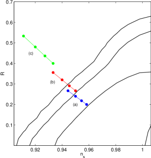
Figure 4: Theoretical prediction of large-field models together with the $1\sigma$, $2\sigma$ and $3\sigma$ observational contour bounds. Each case corresponds to (a) $p=2$, (b) $p=4$ and (c) Exponential potential case ($p\to\infty$), respectively, with $e$-foldings $N=45,50,55,60$ (from top to bottom).

When $p=2$, the inflaton mass $m_{\phi}\equiv\sqrt{2c}$ is constrained from Eq. (39) as

$$m_{\phi}\simeq 5\times 10^{-5}M_{5}\,,$$ (40)

which is different from the case of standard inflation, $m_{\phi}\simeq 10^{-6}m_{{\rm Pl}}$. In the case of $p=4$ the self coupling, $\lambda_{\phi}\equiv 4c$, is constrained to be

$$\lambda_{\phi}\simeq 8.2\times 10^{-15}\,,$$ (41)

which is slightly smaller than the case of standard inflation, $\lambda_{\phi}\simeq 10^{-13}$.

As we have seen the model parameters can be strongly constrained in large-field models. This is due to the fact that we have only one free parameter, $c$, for the potential Eq. (29) and that both $n_{\rm S}$ and $R$ can be written by using the $e$-folding number only even in the presence of the brane tension, $\lambda$.

IV.2 Small-field models

Small-field models are characterized by the condition $\eta<0$, which means that the second derivative of the potential is negative. The potential in these models around the region $\phi=0$ is written in the form

$$V\left(\phi\right)=V_{0}\left[1-\left({\phi/\mu}\right)^{p}\right]\,.$$ (42)

A realistic model would consider a potential that has a local minimum, e.g.,

$$V\left(\phi\right)=V_{0}\left[1-\frac{1}{2}\left(\frac{\phi}{\mu}\right)^{p}\right]^{2}\,,$$ (43)

which is well approximated by the potential Eq. (42) for $|(\phi/\mu)^{p}|\ll 1$.

New inflation is characterized by the potential Eq. (43) with $p=2$. Natural inflation is slightly different from Eq. (43), but it is approximated as Eq. (43) by performing a Taylor expansion around $\phi=0$. The potential of the tachyon field computed in the bosonic string field theory is given by Gerasimov:2000zp ; Bento:2002np

$$V\left(\chi\right)=\tau_{3}\left(\frac{\chi}{\chi_{*}}\right)^{2}\left(1-2\,{\rm ln}\,\frac{\chi}{\chi_{*}}\right)\,,$$ (44)

where $\tau_{3}$ is the D3 brane tension and $\chi_{*}=2l_{\rm s}\sqrt{\tau_{3}}$ with $l_{\rm s}$ being a string-length scale. This potential has a local maximum at $\chi=\chi_{*}$ and inflation is realized around this region ($\chi$ evolves toward the potential minimum at $\chi=0$). We can perform a Taylor expansion around $\chi=\chi_{*}$, which gives an approximate form of the potential

$$V\left(\chi\right)\simeq\tau_{3}\left[1-2\left(\frac{\chi}{\chi_{*}}-1\right)^{2}\right]\,.$$ (45)

This reduces to the potential (42) with $p=2$ by rewriting $\tau_{3}=V_{0}$, $\phi=\chi-\chi_{*}$ and $\chi_{*}^{2}=2\mu^{2}$. Therefore the tachyon potential Eq. (44) belongs to small-field models by shifting the potential maximum to $\phi=0$.

Hereafter we shall consider the potential Eq. (43) and assume the condition $|(\phi/\mu)^{p}|\ll 1$. We obtain $n_{{\rm S}}$ and $R$ from Eqs. (22) and (23) as

$$n_{{\rm S}} \simeq 1-\frac{1}{2\pi}\left(\frac{m_{{\rm Pl}}}{\mu}\right)^{2}\frac{\lambda}{V_{0}}p$$

$$\times \biggl{[}(p-1)\left(\frac{\phi}{\mu}\right)^{p-2}+\left(4p-\frac{3}{2}\right)\left(\frac{\phi}{\mu}\right)^{2(p-1)}\biggr{]}\,,$$

$$R \simeq \frac{6}{\pi}\left(\frac{m_{{\rm Pl}}}{\mu}\right)^{2}\frac{\lambda}{V_{0}}p^{2}\left(\frac{\phi}{\mu}\right)^{2(p-1)}\,,$$ (47)

together with the amplitude of scalar perturbations

$$A_{{\rm S}}^{2}\simeq\frac{64\pi V_{0}^{4}\mu^{2}}{75m_{{\rm Pl}}^{6}\lambda^{3}p^{2}}\left(\frac{\phi}{\mu}\right)^{2(1-p)}\,.$$ (48)

The field value $\phi_{f}$ takes a different form depending on the model parameters. If the condition $r\equiv 5\lambda m_{{\rm Pl}}^{2}p^{2}/(24\pi\mu^{2}V_{0})\ll 1$ is satisfied in Eq. (6), the end of inflation is characterized by $\phi_{f}/\mu\simeq 2^{-1/p}$. This condition is automatically satisfied in the limit $\lambda/V_{0}\to 0$. In the case $r\gg 1$, which is possible for $\mu\ll m_{{\rm Pl}}$, we approximately have $\phi_{f}/\mu\simeq[5\lambda m_{{\rm Pl}}^{2}p^{2}/(24\pi\mu^{2}V_{0})]^{1/2(1-p)}$. Hereafter we shall mainly discuss the case $r\ll 1$ and comment on the case $r\gg 1$ at the end.

IV.2.1 Case of $p=2$

When $p=2$ the field $\phi$ is expressed in terms of the $e$-folds $N$ from Eq. (14)

$$\phi\simeq\phi_{f}\exp\left(-\frac{\lambda m_{{\rm Pl}}^{2}}{2\pi V_{0}\mu^{2}}N\right)\,.$$ (49)

Making use of Eqs. (IV.2), (47) and (48) with $\phi_{f}/\mu\simeq 2^{-1/p}$, we get the following relations

$$R = \frac{128V_{0}^{3}}{25\lambda^{2}m_{{\rm Pl}}^{4}}\frac{1}{A_{\rm S}^{2}}=12xe^{-Nx}\,,$$ (50)

$$n_{\rm S} = 1-\frac{13}{48}R-x\,,$$ (51)

where

$$x\equiv\frac{1}{2\pi}\left(\frac{m_{{\rm Pl}}}{\mu}\right)^{2}\frac{\lambda}{V_{0}}p\,.$$ (52)

Then $R$ has a maximum value $R_{\rm max}=12/eN$ at $x=1/N$, which means that $R_{\rm max}$ is smaller than 0.1 on cosmologically relevant scales ($50\lesssim N\lesssim 60$). Comparing to the observational bounds shown in Fig. 5, we find that the point with maximum $R$ is inside the $1\sigma$ curve.

Using the COBE normalized value $A_{\rm S}\simeq 2\times 10^{-5}$ around $N=55$ with the condition $R\leq 12/eN$, one gets

$$\left(\frac{V_{0}}{\lambda}\right)^{2}\frac{V_{0}}{m_{{\rm Pl}}^{4}}\lesssim 6.3\times 10^{-12}\,.$$ (53)

This condition is violated in the high-energy limit $V_{0}/\lambda\to\infty$, which suggests that the information of the COBE normalization limits the strength $V_{0}/\lambda$.

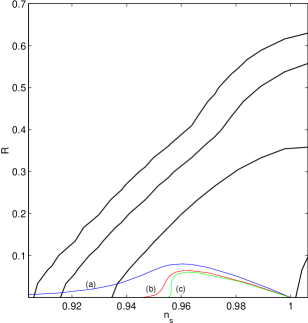
Figure 5: Theoretical prediction of small-field models together with the $1\sigma$, $2\sigma$ and $3\sigma$ observational contour bounds. Each case corresponds to (a) $p=2$, (b) $p=4$ and (c) $p=6$, with $N=55$.

In Fig. 5 we show the two-dimensional plot of $n_{\rm S}$ and $R$ predicted by Eqs. (50) and (51) [see case (a)]. Compared to the 2D posterior observational constraints shown in Fig. 1, theoretical predicted points are inside the $2\sigma$ curve as long as $|n_{\rm S}-1|\lesssim 0.09$. This translates into the condition $x\lesssim 0.09$, i.e.,

$$\left(\frac{m_{{\rm Pl}}}{\mu}\right)^{2}\frac{\lambda}{V_{0}}\lesssim 0.28\,.$$ (54)

If we assume that the mass $\mu$ is smaller than $m_{{\rm Pl}}$, we get the constraints $\lambda/V_{0}\lesssim 0.28$ and $V_{0}/m_{{\rm Pl}}^{4}\lesssim 5.0\times 10^{-13}$ from Eqs. (53) and (54). In natural inflation the typical energy scale is the GUT scale, i.e., $V_{0}\sim(10^{16}\,{\rm GeV})^{4}$, corresponding to $V_{0}/m_{{\rm Pl}}^{4}\sim 10^{-12}$. The above upper limit of the energy scale in the brane case is not much different from the one in standard inflationary cosmology.

IV.2.2 Case of $p>2$

When $p>2$ the terms in the square bracket of Eq. (IV.2) can be much smaller than unity for $|\phi/\mu|\ll 1$. This means that the factor $x$ which appears in front of the square bracket of Eq. (IV.2) is not necessarily required to be smaller than unity in order to be compatible with observations.

The field $\phi$ is written as

$$\left(\frac{\phi}{\mu}\right)^{2-p}=\frac{\lambda m_{{\rm Pl}}^{2}p(p-2)N}{4\pi V_{0}\mu^{2}}+\left(\frac{\phi_{f}}{\mu}\right)^{2-p}\,.$$ (55)

Let us first consider the case of $x\ll 1$ and $\phi_{f}/\mu\simeq 2^{-1/p}$. Then we can express $R$ and $n_{\rm S}$ in terms of $x$:

$$R = \frac{128V_{0}^{3}}{25\lambda^{2}m_{{\rm Pl}}^{4}}\frac{1}{A_{\rm S}^{2}}$$ (56)

$$= 12px\left(\frac{(p-2)Nx}{2}+2^{1-\frac{2}{p}}\right)^{\frac{2(p-1)}{2-p}}\,,$$

$$n_{\rm S} = 1-\left(\frac{1}{3}-\frac{1}{8p}\right)R$$ (57)

$$-\frac{2(p-1)x}{(p-2)Nx+2^{2(1-1/p)}}\,.$$

Notice that $R$ is written in terms of $A_{\rm S}^{2}$ independent of the values of $p$. The maximum value $R_{\rm max}$ gets gradually smaller with the increase of $p$. When $p=4$, for example, one has $R_{\rm max}\simeq 0.065$ for $N\simeq 55$, thereby yielding

$$\left(\frac{V_{0}}{\lambda}\right)^{2}\frac{V_{0}}{m_{{\rm Pl}}^{4}}\lesssim 5.1\times 10^{-12}\,.$$ (58)

Figure 5 indicates that the theoretical curves do not lie in the region $n_{\rm S}\lesssim 0.94$ even with the increase in the value of $x$. Let us consider the case with $x\gg 1$ (corresponding to $r\gg 1$). Since $\phi_{f}$ is estimated as $\phi_{f}/\mu\simeq[5\lambda m_{{\rm Pl}}^{2}p^{2}/(24\pi\mu^{2}V_{0})]^{1/2(1-p)}$ in this case, we have

$$R = 12px\left\{\frac{(p-2)Nx}{2}+\left(\frac{5px}{12}\right)^{\frac{2-p}{2(1-p)}}\right\}^{\frac{2(p-1)}{2-p}}\!\!\!\!\!\!,$$ (59)

$$n_{\rm S} = 1-\left(\frac{1}{3}-\frac{1}{8p}\right)R$$ (60)

$$-\frac{2(p-1)x}{(p-2)Nx+2(5px/12)^{\frac{2-p}{2(1-p)}}}\,.$$

In the limit $x\to\infty$, we find $R\propto x^{p/(2-p)}\to 0$ and

$$n_{\rm S}\to 1-\frac{2(p-1)}{(p-2)N}\,.$$ (61)

When $N=55$ one has $n_{\rm S}\to 0.946$ for $p=4$ and $n_{\rm S}\to 0.955$ for $p=6$. As seen in Fig. 5, the curves predicted by Eqs. (56) and (57) are inside the $1\sigma$ curve. Therefore the model parameters are less constrained than in the case of $p=2$. This is associated with the fact that the potential becomes flat around $\phi=0$ for larger values of $p$, which does not exhibit strong deviation from $n_{\rm S}=1$ and $R=0$.

IV.3 Hybrid models

Hybrid inflation is motivated by particle physics models which involve supersymmetry. The potential of the original hybrid inflation proposed by Linde is given as hybrid

$$V=\frac{\lambda_{0}}{4}\left(\chi^{2}-\frac{M^{2}}{\lambda_{0}}\right)^{2}+\frac{1}{2}g^{2}\phi^{2}\chi^{2}+\frac{1}{2}m^{2}\phi^{2}\,.$$ (62)

The supersymmetric scenario corresponds to $g^{2}=2\lambda_{0}$ hybrid2 ; Lyth:1998xn , which is the case we shall consider hereafter. Inflation occurs for $\phi>\phi_{f}\equiv M/g$, which is followed by the symmetry breaking driven by a second scalar field, $\chi$. When the “waterfall” condition, $M^{3}\ll\lambda_{0}mm_{{\rm Pl}}^{2}$, is satisfied, inflation soon comes to an end after the symmetry breaking hybrid . This corresponds to the original version of the hybrid inflationary scenario where inflation ends due to the rapid rolling of the field $\chi$. Setting $\chi\simeq 0$ in Eq. (62), the effective potential for $\phi>\phi_{f}$ is written as

$$V\simeq\frac{M^{4}}{4\lambda_{0}}+\frac{1}{2}m^{2}\phi^{2}\,.$$ (63)

Notice that the second phase of inflation occurs after the symmetry breaking when the waterfall condition is not satisfied. This corresponds to a double inflationary scenario in which the second stage of inflation can affect the evolution of cosmological perturbations. In fact, as shown in Ref. Tsujikawa:2002qx , the presence of the tachyonic instability for $\phi<\phi_{f}$ leads to the strong correlation between adiabatic and isocurvature perturbations, which can affect the CMB power spectrum.

In this work we shall consider the case where perturbations on cosmologically-relevant scales are generated before the symmetry breaking and also neglect the contribution of isocurvature perturbations. Then the general hybrid inflation is given in the form

$$V\left(\phi\right)=V_{0}\left[1+\left({\phi/\mu}\right)^{p}\right]\,,$$ (64)

which correspond to the parameter range of $\eta>\epsilon$ for $V/\lambda\gg 1$. For the potential Eq. (63) we have three model parameters, $\lambda_{0}$, $M$ and $m$. Note that $\phi_{f}$ is expressed in terms of $\lambda_{0}$ and $M$, as $\phi_{f}=M/\sqrt{2\lambda_{0}}$. This is equivalent to considering three parameters, $V_{0}$, $\mu$ and $\phi_{f}$ for the potential Eq. (64). Since we have one additional parameter compared to small-field models, it is expected that constraining the model is more difficult in this case.

However one has additional constraints on $V_{0}$ and $\mu$ in realistic supergravity models. We can consider the following supergravity-motivated cases hybrid2 ; Linde:1997sj (corresponding to $p=2$ and $p=4$, respectively)

$${\rm(i)}~{}~{}V(\phi) = V_{0}\left[1+8\pi\left(\frac{\phi}{m_{{\rm Pl}}}\right)^{2}\right]\,,$$ (65)

$${\rm(ii)}~{}~{}V(\phi) = V_{0}\left[1+8\pi^{2}\left(\frac{\phi}{m_{{\rm Pl}}}\right)^{4}\right]\,.$$ (66)

In case (i) the second slow-roll parameter is given as $\eta=2/(1+V/2\lambda)$. Then we have $\eta=2$ in the low-energy limit, which makes it difficult to achieve inflation (the so-called $\eta$-problem). This problem is overcome in the braneworld, since $\eta\to 0$ for $V/\lambda\to\infty$. The case (ii) corresponds to inclusion of the supergravity corrections to the effective potential in a globally-supersymmetric theory Linde:1997sj (we neglected one-loop radiative corrections calculated in Ref. Linde:1997sj ). We have $\eta=12\pi(\phi/m_{{\rm Pl}})^{2}/(1+V/2\lambda)$ in this case, which means that inflation is possible even in the low-energy limit as long as $\phi\ll m_{{\rm Pl}}$.

We shall first consider the general potential Eq. (64) without imposing the supergravity relations. When $(\phi_{f}/\mu)^{p}$ is larger than unity in Eq. (64), this is not much different from large-field models discussed in subsection A. Therefore the condition $|(\phi/\mu)^{p}|\ll 1$ is assumed hereafter, in which case we have

$$n_{{\rm S}} \simeq 1+\frac{1}{2\pi}\left(\frac{m_{{\rm Pl}}}{\mu}\right)^{2}\frac{\lambda}{V_{0}}p$$

$$\times\biggl{[}(p-1)\left(\frac{\phi}{\mu}\right)^{p-2}+\left(2-5p\right)\left(\frac{\phi}{\mu}\right)^{2(p-1)}\biggr{]}\,,$$

where $R$ and $A_{\rm S}^{2}$ take the same forms as in Eqs. (47) and (48), thereby yielding

$$R=\frac{128V_{0}^{3}}{25\lambda^{2}m_{{\rm Pl}}^{4}}\frac{1}{A_{\rm S}^{2}}\,.$$ (68)

The observational constraint imposes the condition $R\lesssim 0.57$ from Fig. 1, yielding

$$\left(\frac{V_{0}}{\lambda}\right)^{2}\frac{V_{0}}{m_{{\rm Pl}}^{4}}\lesssim 4.5\times 10^{-11}\,.$$ (69)

This is a general prediction of hybrid and small-field models. Note that this value is more tightly constrained in small-field models as we showed in the previous subsection, but the hybrid models are somewhat different because of the additional model parameter.

Hereafter we consider the cases of $p=2$ and $p>2$ separately.

IV.3.1 Case of $p=2$

In this case $\phi$, $R$ and $n_{\rm S}$ are expressed as

$$\phi = \phi_{f}\exp\left(\frac{\lambda m_{{\rm Pl}}^{2}}{2\pi V_{0}\mu^{2}}N\right)\,,$$ (70)

$$R = 24(\phi_{f}/\mu)^{2}xe^{Nx}\,,$$ (71)

$$n_{\rm S} = 1+x\left[1-8(\phi_{f}/\mu)^{2}e^{Nx}\right]\,,$$ (72)

where $x$ is defined in Eq. (52).

In Fig. 6 we plot the above relations for several different values of $\phi_{f}/\mu$. When $\phi_{f}/\mu\lesssim 10^{-3}$ the theoretical curve is outside of the $2\sigma$ contour bound unless $x$ ranges $0\leq x\lesssim 0.05$ (note that $R$ is much smaller than 1 for $0\leq x\lesssim 0.05$ in the case (a) of Fig. 6). Therefore one gets the following constraint

$$\left(\frac{m_{{\rm Pl}}}{\mu}\right)^{2}\frac{\lambda}{V_{0}}\lesssim 0.16\,,~{}~{}{\rm for}~{}~{}\phi_{f}/\mu\lesssim 10^{-3}\,.$$ (73)

The supergravity potential (65) corresponds to $\mu=m_{{\rm Pl}}/\sqrt{8\pi}$, which yields the constraint $\lambda/V_{0}\lesssim 6.3\times 10^{-3}$ from Eq. (73). Making use of Eq. (69), we have a bound on the energy scale of inflation, $V_{0}/m_{{\rm Pl}}^{4}\lesssim 1.6\times 10^{-14}$. This is about $10^{-2}$ times lower than the GUT scale, $V_{0}/m_{{\rm Pl}}^{4}\sim 10^{-12}$.

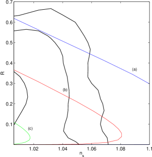
Figure 6: Theoretical prediction of hybrid models together with the $1\sigma$, $2\sigma$ and $3\sigma$ observational contour bounds. Each case corresponds to (a) $\phi_{f}/\mu=10^{-3}$, (b) $\phi_{f}/\mu=10^{-2}$ and (c) $\phi_{f}/\mu=10^{-1}$ with $N=55$.

When $\phi_{f}/\mu\gtrsim 10^{-3}$, Fig. 6 indicates that the theoretical curves begin to be within the likelihood contour bounds. In particular the curve is completely inside the $2\sigma$ bound for $\phi_{f}/\mu\gtrsim 0.03$, thus favoured observationally. However we have one thing that must be considered with care. There is a turnover for $n_{\rm S}$ coming from the second term in the square bracket of Eq. (IV.3). Since we used the condition $(\phi_{f}/\mu)^{2}\ll 1$ to derive this formula, Eq. (IV.3) is not valid when $n_{\rm S}$ reaches close to 1 with the increase of $x$, corresponding to $x_{\rm M}=(2/N){\rm log}(\mu/2\sqrt{2}\phi_{f})$. The rough criterion for the validity of the approximation is $x\lesssim x_{\rm M}$, implying

$$\left(\frac{m_{{\rm Pl}}}{\mu}\right)^{2}\frac{\lambda}{V_{0}}\lesssim\frac{2\pi}{N}\,{\rm log}\left(\frac{\mu}{2\sqrt{2}\phi_{f}}\right)\,.$$ (74)

This comes from the requirement for hybrid inflation $((\phi_{f}/\mu)^{p}\ll 1)$ so that the potential energy $V_{0}$ dominates in Eq. (64). For the supergravity potential (65) with $N=55$, one gets $\lambda/V_{0}\lesssim 4.5\times 10^{-3}{\rm log}\,(\mu/(2\sqrt{2}\phi_{f}))$. When $\phi_{f}/\mu\gtrsim 0.03$, this yields $\lambda/V_{0}\lesssim 1.2\times 10^{-2}$. Inflation is realized in the high-energy regime (corresponding to small $\lambda/V_{0}$) in this case, which gives the values of $n_{\rm S}$ and $R$ close to $n_{\rm S}=1$ and $R=0$.

IV.3.2 Case of $p>2$

When $p>2$ we have

$$\left(\frac{\phi}{\mu}\right)^{2-p} = \left(\frac{\phi_{f}}{\mu}\right)^{2-p}-\frac{(p-2)Nx}{2}\,,$$ (75)

$$R = 12px\left[\left(\frac{\phi_{f}}{\mu}\right)^{2-p}-\frac{(p-2)Nx}{2}\right]^{\frac{2(p-1)}{2-p}}\!\!\!\!\!\!,$$ (76)

$$n_{\rm S}-1 = (p-1)x\left(\frac{R}{12px}\right)^{\frac{p-2}{2(p-1)}}+\frac{2-5p}{12p}R\,.$$ (77)

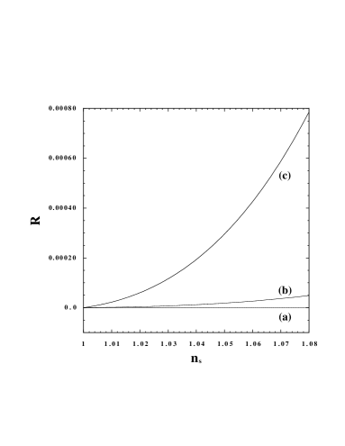
Figure 7: Theoretical prediction for $n_{\rm S}$ and $R$ in hybrid inflation models for $p=4$. Each case corresponds to (a) $\phi_{f}/\mu=10^{-2}$, (b) $\phi_{f}/\mu=5\times 10^{-2}$ and (c) $\phi_{f}/\mu=10^{-1}$ with $N=55$.

Under the condition of $|\phi_{f}/\mu|\ll 1$, the ratio $R$ is much smaller than unity (see Fig. 7). This means that we only need to consider the constraint on $n_{\rm S}$. The spectral index is approximately written as $n_{\rm S}-1\simeq(p-1)x/[(\phi_{f}/\mu)^{2-p}-(p-2)Nx/2]$ for $|(\phi_{f}/\mu)^{p}|\ll 1$. We have the $2\sigma$ constraint $n_{\rm S}\lesssim 1.05$ for $R\ll 1$ from Fig. 6, which leads to

$$x\lesssim\frac{0.05(\phi_{f}/\mu)^{2-p}}{(p-1)+0.025(p-2)N}\,.$$ (78)

In the case of $p=4$ with $N=55$, this reduces to

$$\left(\frac{m_{{\rm Pl}}}{\mu}\right)^{2}\frac{\lambda}{V_{0}}\lesssim 2.6\times 10^{-2}\left(\frac{\mu}{\phi_{f}}\right)^{2}\,.$$ (79)

The supergravity potential Eq. (66) corresponds to $\mu^{2}=m_{{\rm Pl}}^{2}/(\sqrt{8}\pi)$, in which case the condition Eq. (79) is simplified as

$$\frac{\lambda}{V_{0}}\lesssim 2.9\times 10^{-3}\left(\frac{\mu}{\phi_{f}}\right)^{2}\,.$$ (80)

Combining Eq. (69) with Eq. (80), we get the constraint

$$\frac{V_{0}}{m_{{\rm Pl}}^{4}}\lesssim 3.5\times 10^{-16}\left(\frac{\mu}{\phi_{f}}\right)^{4}\,,$$ (81)

whose upper bound is dependent on the value $\phi_{f}/\mu$.

V Summary and Discussions

In this paper we have investigated observational constraints on the Randall-Sundrum type II braneworld inflationary models. The consistency relation Eq. (16) holds independent of the strength of the brane tension $\lambda$, so that the same likelihood analysis can be employed as for standard inflationary models. We carried out the likelihood analysis by varying the inflationary parameters as well as other cosmological parameters. We take into account several independent cosmological datasets including the latest SDSS galaxy redshift survey SDSS , and show that this leads to a tight constraint on the values of $n_{\rm S}$ and $R$ relative to including WMAP data alone Barger:2003ym . Our results are also consistent with the likelihood analysis of the SDSS group Tegmark . We also point out the importance of putting an appropriate prior for the running of scalar perturbations, which otherwise leads to an unexpected shift toward larger likelihood values of $R$.

In braneworld the constraints on model parameters in terms of the underlying potentials are different compared to standard inflation. We classified the models of inflation as large-field, small-field and hybrid models, and constrained the model parameters for each case. In large-field models, which have only one free parameter in the potential, both $n_{\rm S}$ and $R$ are the function in terms of the $e$-folds $N$ only. This simple property allows us to place strong constraints on large-field models. While the quadratic potential is within the observational $2\sigma$ bound for $N\gtrsim 50$, the quartic potential is disfavoured since the predicted curve is outside the $2\sigma$ bound for $N<60$ (see Fig. 4). The steep inflation driven by an exponential potential is far outside the $3\sigma$ bound, thus excluded observationally.

In small-field models one has an additional parameter associated with the potential, which implies that it is more difficult to constrain model parameters compared to large-field models. In spite of this, we can place an upper bound on the energy scale of inflation using the information of $A_{\rm S}^{2}$ and $R$, see Eqs. (53) and (58). The $p=2$ case for the potential Eq. (43) is not excluded as long as the condition Eq. (54) is satisfied. The $p>2$ case does not possess additional restrictions on model parameters, since the theoretical prediction is within the $1\sigma$ contour bound (see Fig. 5).

Hybrid models are more involved due to the fact that there is one more additional parameter associated with the end of inflation ($\phi_{f}$). Nevertheless we placed limits on the energy scale of inflation and also obtained the relationship between $\mu,\lambda/V_{0}$ and $\phi_{f}$ from observational bounds in the $n_{\rm S}$–$R$ plane [see Eqs. (69), (74) and (79)]. These relations can be simplified in supergravity models due to an additional relation between $V_{0}$ and $\mu$.

Although the constraint on each inflation model in braneworld differs from the one in standard inflationary cosmology, the likelihood values of inflationary parameters ($A_{\rm S}$, $R$, $n_{\rm S}$, $n_{\rm T}$, $\alpha_{\rm S}$, $\alpha_{\rm T}$) are the same in both cases. In order to pick up the signature of braneworld, it is required to break through the degeneracy of the consistency relation. This degeneracy is associated with the fact that 5-dimensional observables smoothly approach the 4-dimensional counterpart in an exact de-Sitter embedding, as we decouple the brane from the bulk with an increasing brane tension. However it was recently shown in Ref. Seery that this does not hold for a marginally-perturbed de-Sitter geometry and the relationship between observables is dependent on the brane tension (see also Ref. Calcagni ). This can provide one possible way to distinguish between braneworld and standard inflation from different constraints on observables.

While we concentrated on single-field inflationary scenarios in this work, the CMB power spectrum is generally modified if isocurvature perturbations dominate adiabatic ones Langlois . In the low-energy case the correlation between adiabatic and isocurvature perturbations is strong for the double inflation model with potential given by Eq. (62) Tsujikawa:2002qx . When the second stage of inflation occurs after the symmetry breaking, it is important to follow the dynamics of curvature perturbations ${\cal R}$ precisely, since ${\cal R}$ is no longer conserved in the context of multi-field inflation multi . The enhancement of curvature perturbations reduces the relative amplitude of tensor to scalar perturbations, which leads to the modified consistency relation Bartolo

$$R=-8n_{\rm T}(1-r_{C}^{2})\,,$$ (82)

where $r_{C}$ is the correlation between adiabatic and isocurvature perturbations. Although it is not obvious whether the same consistency relation holds or not in braneworld, especially when the second scalar field corresponds to the brane modulus, it would be interesting to find out the signature of braneworld in such generic cases. See Ref. Ashcroft for recent work in this direction.

In this paper we have only considered braneworld effects on generating the initial power spectra, while in general there may be 5D effects at late times impacting on, for example, CMB anisotropies. Recently there have been several attempts to give a quantitative prediction of the CMB power spectrum by solving a bulk geometry using a low-energy approximation Kanno in a two-brane system Koyama:2003be ; Rhodes:2003ev . While this approach involves some unresolved issues such as the stabilization of the modulus (radion), this is the first important step to understand the effect of the 5D perturbations. In particular it was shown in Ref. Koyama:2003be that the effect of the Weyl anisotropic stress leads to the modification of the CMB temperature anisotropy around the first doppler peak, while the perturbations on larger scales are not altered. It would be certainly of interest to extend this analysis to the high-energy regime in order to fully pick up the effect of extra dimensions on CMB anisotropies. We hope that this will open up a possibility to distinguish the braneworld scenario from other inflationary models motivated by, e.g., quantum gravity QG or noncommutative geometry noncominf .

- (1) D. N. Spergel et al., Astrophys. J. Suppl. 148, 175 (2003) [arXiv:astro-ph/0302209].
- (2) H. V. Peiris et al., Astrophys. J. Suppl. 148, 213 (2003) [arXiv:astro-ph/0302225].
- (3) S. L. Bridle, A. M. Lewis, J. Weller, and G. Efstathiou, Mon. Not. Roy. Astron. Soc. 342, L72 (2003) [arXiv:astro-ph/0302306].
- (4) V. Barger, H. S. Lee, and D. Marfatia, Phys. Lett. B 565, 33 (2003) [arXiv:hep-ph/0302150].
- (5) W. H. Kinney, E. W. Kolb, A. Melchiorri, and A. Riotto, [arXiv:hep-ph/0305130].
- (6) S. M. Leach and A. R. Liddle, Phys. Rev. D 68, 123508 (2003) [arXiv:astro-ph/0306305].
- (7) M. Tegmark et al. [SDSS Collaboration], arXiv:astro-ph/0310723.
- (8) L. Randall and R. Sundrum, Phys. Rev. Lett. 83, 4690 (1999) [arXiv:hep-th/9906064].
- (9) A. R. Liddle and A. N. Taylor, Phys. Rev. D 65, 041301 (2002) [arXiv:astro-ph/0109412].
- (10) A. R. Liddle and A. J. Smith, Phys. Rev. D 68 (2003) 061301 [arXiv:astro-ph/0307017].
- (11) M. Tegmark et al. [SDSS Collaboration], arXiv:astro-ph/0310725.
- (12) T. Shiromizu, K. Maeda, and M. Sasaki, Phys. Rev. D 62, 024012 (2000) [arXiv:gr-qc/9910076].
- (13) K. Koyama, Phys. Rev. Lett. 91, 221301 (2003) [arXiv:astro-ph/0303108].
- (14) R. Maartens, D. Wands, B. A. Bassett, and I. Heard, Phys. Rev. D 62, 041301 (2000) [arXiv:hep-ph/9912464].
- (15) S. Tsujikawa, K. Maeda, and S. Mizuno, Phys. Rev. D 63, 123511 (2001) [arXiv:hep-ph/0012141].
- (16) D. Langlois, R. Maartens, and D. Wands, Phys. Lett. B 489, 259 (2000) [arXiv:hep-th/0006007].
- (17) G. Huey and J. E. Lidsey, Phys. Lett. B 514, 217 (2001) [arXiv:astro-ph/0104006].
- (18) D. J. Schwarz, C. A. Terrero-Escalante, and A. A. García, Phys. Lett. B 517, 243 (2001), [arXiv:astro-ph/0106020].
- (19) S. M. Leach, A. R. Liddle, J. Martin, and D. J. Schwarz, Phys. Rev. D 66, 023515 (2002) [arXiv:astro-ph/0202094]; S. M. Leach and A. R. Liddle, Mon. Not. Roy. Astron. Soc. 341, 1151 (2003) [arXiv:astro-ph/0207213].
- (20) A. Lewis, A. Challinor, and A. Lasenby, Astrophys. J. 538, 473 (2000) [arXiv:astro-ph/9911177].
- (21) A. Lewis and S. Bridle, Phys. Rev. D 66, 103511 (2002) [arXiv:astro-ph/0205436]; see also http://camb.info/.
- (22) http://lambda.gsfc.nasa.gov/
- (23) K. Grainge et al., Mon. Not. Roy. Astron. Soc. 341, L23 (2003) [arXiv:astro-ph/0212495].
- (24) T. J. Pearson et al., Astrophys. J. 591, 556 (2003) [arXiv:astro-ph/0205388].
- (25) C. L. Kuo et al., Astrophys. J. 600, 32 (2004) [astro-ph/0212289].
- (26) W. J. Percival et al., Mon. Not. Roy. Astron. Soc. 327, 1297 (2001) [arXiv:astro-ph/0105252].
- (27) J. E. Lidsey, A. R. Liddle, E. W. Kolb, E. J. Copeland, T. Barreiro, and M. Abney, Rev. Mod. Phys. 69, 373 (1997) [arXiv:astro-ph/9508078].
- (28) E. W. Kolb, arXiv:hep-ph/9910311.
- (29) A. Linde, Phys. Lett. 129B, 177 (1983).
- (30) A. Linde, Phys. Lett. 108B, 389 (1982); A. Albrecht and P. Steinhardt, Phys. Rev. Lett. 48, 1220 (1982).
- (31) K. Freese, J. A. Frieman, and A. V. Olinto, Phys. Rev. Lett. 65, 3233 (1990).
- (32) A. D. Linde, Phys. Rev. D 49, 748 (1994) [arXiv:astro-ph/9307002].
- (33) E. J. Copeland, A. R. Liddle, D. H. Lyth, E. D. Stewart, and D. Wands, Phys. Rev. D 49, 6410 (1994) [arXiv:astro-ph/9401011].
- (34) E. J. Copeland, A. R. Liddle, and J. E. Lidsey, Phys. Rev. D 64, 023509 (2001) [arXiv:astro-ph/0006421].
- (35) A. A. Gerasimov and S. L. Shatashvili, JHEP 0010, 034 (2000) [arXiv:hep-th/0009103].
- (36) M. C. Bento, O. Bertolami, and A. A. Sen, Phys. Rev. D 67, 063511 (2003) [arXiv:hep-th/0208124].
- (37) D. H. Lyth and A. Riotto, Phys. Rept. 314, 1 (1999) [arXiv:hep-ph/9807278].
- (38) S. Tsujikawa, D. Parkinson, and B. A. Bassett, Phys. Rev. D 67, 083516 (2003) [arXiv:astro-ph/0210322].
- (39) A. D. Linde and A. Riotto, Phys. Rev. D 56, 1841 (1997) [arXiv:hep-ph/9703209].
- (40) D. Seery and A. Taylor, arXiv:astro-ph/0309512.
- (41) G. Calcagni, arXiv:hep-ph/0312246.
- (42) D. Langlois, Phys. Rev. D 59, 123512 (1999) [arXiv:astro-ph/9906080]; L. Amendola, C. Gordon, D. Wands, and M. Sasaki, Phys. Rev. Lett. 88, 211302 (2002) [arXiv:astro-ph/0107089]; J. Valiviita and V. Muhonen, Phys. Rev. Lett. 91, 131302 (2003) [arXiv:astro-ph/0304175]; P. Crotty, J. Garcia-Bellido, J. Lesgourgues, and A. Riazuelo, Phys. Rev. Lett. 91, 171301 (2003) [arXiv:astro-ph/0306286].
- (43) A. A. Starobinsky and J. Yokoyama, arXiv:gr-qc/9502002; J. Garcia-Bellido and D. Wands, Phys. Rev. D 53, 5437 (1996) [arXiv:astro-ph/9511029]; S. Tsujikawa and H. Yajima, Phys. Rev. D 62, 123512 (2000) [arXiv:hep-ph/0007351]; A. A. Starobinsky, S. Tsujikawa, and J. Yokoyama, Nucl. Phys. B 610, 383 (2001) [arXiv:astro-ph/0107555]; S. Tsujikawa and B. A. Bassett, Phys. Lett. B 536, 9 (2002) [arXiv:astro-ph/0204031].
- (44) N. Bartolo, S. Matarrese, and A. Riotto, Phys. Rev. D 64, 123504 (2001) [arXiv:astro-ph/0107502]; D. Wands, N. Bartolo, S. Matarrese, and A. Riotto, Phys. Rev. D 66, 043520 (2002) [arXiv:astro-ph/0205253].
- (45) P. R. Ashcroft, C. van de Bruck, and A. C. Davis, arXiv:astro-ph/0310643.
- (46) S. Kanno and J. Soda, Phys. Rev. D 66, 043526 (2002) [arXiv:hep-th/0205188].
- (47) C. S. Rhodes, C. van de Bruck, P. Brax and A. C. Davis, Phys. Rev. D 68, 083511 (2003) [arXiv:astro-ph/0306343].
- (48) M. Bojowald, Phys. Rev. Lett. 89, 261301 (2002) [arXiv:gr-qc/0206054]; M. Bojowald and K. Vandersloot, Phys. Rev. D 67, 124023 (2003) [arXiv:gr-qc/0303072]; S. Tsujikawa, P. Singh, and R. Maartens, arXiv:astro-ph/0311015.
- (49) S. Alexander, R. Brandenberger, and J. Magueijo, Phys. Rev. D 67, 081301 (2003) [arXiv:hep-th/0108190]; Q. G. Huang and M. Li, JHEP 0306, 014 (2003) [arXiv:hep-th/0304203]; S. Tsujikawa, R. Maartens, and R. Brandenberger, Phys. Lett. B 574, 141 (2003) [arXiv:astro-ph/0308169].