Resolving the Stellar Population of the Standard Elliptical Galaxy NGC3379

Abstract

Using the Near Infrared Camera and Multi-Object Spectrometer (NICMOS) on board the Hubble Space Telescope, we have obtained $F110W$ ($\sim J$) and $F160W$ ($\sim H$) images of three fields in NGC3379, a nearby normal giant elliptical galaxy. These images resolve individual red giant stars, yielding the first accurate color-magnitude diagrams for a normal luminous elliptical. The photometry reaches $\sim$ 1 magnitude below the red giant branch tip with errors of $\lesssim 0.2$ mags in $F110W-F160W$. A strong break in the luminosity function at $F160W=23.68\pm 0.06$ is identified as the tip of the red giant branch (RGB); comparison with theoretical isochrones implies a distance of $10.8\pm 0.6$ Mpc, in good agreement with a number of previous estimates using various techniques. The mean metallicity is close to solar, but there is an appreciable spread in abundance, from at least as metal poor as [Fe/H]$\approx-1.5$ to as high as $+0.8$. There is a significant population of stars brighter than the RGB tip by up to $\sim 1$ magnitude. The observations of each field were split over two epochs, separated by $2-3$ months, allowing the identification of candidate long period variables; at least $40\%$ of the stars brighter than the RGB tip are variable. Lacking period determinations, the exact nature of these variables remains uncertain, but the bright AGB stars and variables are similar to those found in metal rich globular clusters and are not luminous enough to imply an intermediate age population. All of the evidence points to a stellar population in NGC3379 which is very similar to the bulge of the Milky Way, or an assortment of Galactic globular clusters covering a large metallicity spread.

1 Introduction

Knowledge of the present stellar content and star formation histories of early type galaxies is essential for theories of galaxy evolution and has important consequences for the use of ellipticals in the distance ladder. A major barrier to divining the nature of luminous elliptical galaxies is the dearth of nearby examples whose stellar populations can be resolved and studied star-by-star. Consequently, considerable effort has been expended in spectral synthesis modeling of the integrated light of early type galaxies (e.g. Leitherer, et al. 1996), but spectral modeling has not yet clarified the nature of the stellar population of normal giant elliptical galaxies. There is often significant disagreement over even the most fundamental issues of mean age and metallicity among various methods, as was documented by Arimoto (1996) in a blind test of many spectral synthesis methods by independent researchers. Resolved stellar population analyses of elliptical galaxies is essential for making real progress.

Ground-based color-magnitude diagrams (CMDs) in the near-infrared by Freedman (1989; 1992) and Elston & Silva (1992) for the Local Group high surface brightness, compact dwarf elliptical M32 (NGC221) appeared to exhibit an excess of stars well above the tip of the red giant branch (RGB), evidence for an intermediate age population. More recent V-I CMDs from the Hubble Space Telescope (HST) using WFPC2 (Grillmair et al. 1996), however, find no direct evidence for this population, apparently an artifact of crowding in the ground-based studies, as was predicted by Renzini (1992). After M32, the next nearest early type galaxy stand-in is the spheroid of NGC5128. Soria et al. (1996), Harris et al. (1999), and Marleau et al. (2000) have constructed CMDs using HST WFPC2 V + I or NICMOS J + H images of the outer halo of NGC5128, detecting the tip of the RGB and plentiful bright asymptotic giants, the latter strongly suggesting an intermediate age population. Maffei 1, at a distance of $\sim 4$ Mpc (Luppino & Tonry 1993), is probably the nearest normal elliptical galaxy (Buta & McCall 2003), but at a Galactic latitude of $-0\fdg 55$, it is severely obscured by large and highly variable Galactic extinction, $A_{V}\approx 5$, making it a very difficult object for study at optical and IR wavelengths. Using ground-based adaptive optics, Davidge (2002) has resolved AGB stars in Maffei 1 in the $H$ and $K$ bands, reaching $K\approx 22$ with errors of $0.25$ magnitudes, but not yet good enough to detect the RGB tip or study the RGB population in detail.

These results are important for understanding early type galaxy populations, but neither M32 nor NGC5128 is a normal, luminous, elliptical galaxy. With M${}_{\rm V}=-16$, M32 is at the low luminosity extreme of high surface brightness ellipticals and its proximity to M31 has almost certainly influenced its development (Faber 1973; Nieto & Prugniel 1983; Bekki et al. 2001). NGC5128 is quite peculiar, a probable recent merger harboring an active galaxy nucleus (Soria et al. 1996) and stars as young as 10 Myr (Rejkuba et al. 2001; 2002). Study of Maffei 1 is greatly complicated and compromised by the variable foreground Galactic dust across its field. Color-magnitude diagrams for these unusual objects cannot, without further investigation, be considered representative of the class of standard, luminous ellipticals.

The nearest normal giant elliptical galaxy which can be studied free of complications is NGC3379 in the Leo I galaxy group. It is an E0, with typical early type colors, Mg₂ index, and velocity dispersion (Davies et al. 1987). It is well fit by an R${}^{\text@frac{1}{4}}$ law (de Vaucouleurs & Capaccioli 1979) and appears to have no large scale morphological peculiarities (Schweizer and Seitzer 1992). There is some evidence that NGC3379 could be a face-on S0 (Statler & Smecker-Hane 1999; Capaccioli et al. 1991), but the evidence is equivocal. It contains a tiny nuclear dust ring, $R\approx 1\farcs 5$, and small ionized gas ring, $R\approx 8$ (Pastoriza et al. 2000; Statler 2001). This amount of visible interstellar material is small compared to that in the 40% of typical bright ellipticals with gas and dust (Faber et al. 1997; Sadler & Gerhard 1985). The Leo I group, which also includes the S0 NGC3384 and the Sc NGC3389, is distinguished by its large partial ring of neutral hydrogen (Schneider 1989).

The HST Extragalactic Distance Scale Key Project (Freedman et al. 2001) arrives at a distance of $\sim 9.5$ Mpc ($m-M=29.90\pm 0.10$) for the Leo I group, somewhat lower than most other estimates (Tanvir et al. 1999, Graham et al. 1997; Tonry et al. 1990; Sakai, Freedman, & Madore 1996; see Gregg 1997 for a short summary). At this distance, the resolved stellar population of NGC3379 is all but impossible to study with present ground-based instrumentation. Sakai et al. (1996) used WFPC2 to obtain I-band images just deep enough to locate the tip of the RGB in NGC 3379 in a field $5-6\arcmin$ from the center. While providing a distance estimate of $11.5\pm 1.6$ Mpc ($m-M=30.30\pm 0.14$), marginally consistent with the Key Project distance, their single filter observations do not constrain the metallicity of the RGB or probe the nature of the AGB.

Apart from the detection of the RGB tip (TRGB) by Sakai et al., everything that is known about the stellar population of NGC3379 has been inferred from spectroscopy and photometry of its integrated light. Compiling the spectral line data from a number of recent studies, Terlevich & Forbes (2002) have derived age and metallicity estimates for 150 nearby elliptical galaxies, using the stellar population models of Worthey & Ottaviani (1997). The mean results for NGC3379 indicate values of $t=9.3$ Gyr and [Fe/H] $=+0.16$, [Mg/Fe] $=+0.24$, consistent with its having a canonical old, relatively metal-rich stellar population. Rose (1985), however, has presented arguments based on detailed analysis of integrated light spectral line strengths, that luminous ellipticals, NGC3379 included, have a “substantial” intermediate age component, $6-7$ Gyr old, though the fraction is not quantified. These conclusions from integrated spectra are based on single-metallicity population models and so must be viewed with some reservations; NGC3379, like most ellipticals, exhibits line strength and color gradients (Davies, Sadler, & Peletier 1993), indicative of abundance variations (Peletier et al. 1999) and hence a composite metallicity population. A metal-poor component can plausibly account for the relatively young turnoff age reported by Rose (1985).

Using HST with NICMOS Camera 2 (Thompson et al. 1998), we have resolved the bright RGB and AGB stars in three fields in the halo of NGC3379 in the $F110W$ ($\sim J$) and $F160W$ ($\sim H$) filters. These images have yielded CMDs, the first such data for a normal, luminous elliptical galaxy which probe below the RGB tip with some precision. Analysis of these data allow us to place constraints on the mean metallicity of the giant stars and to compare the CMDs to those for nearer, relatively well-observed early type populations, such as the Milky Way bulge and globular clusters, as a first attempt in understanding the star formation history of a typical bright, normal elliptical. By dividing our NICMOS observations into two epochs separated by many weeks, we have identified candidate variable stars in its halo, opening another window on elliptical galaxy stellar populations.

The analysis is summarized as follows: the $F160W$ luminosity function yields the TRGB apparent magnitude ($\S 5.1$). Comparison of the CMD to theoretical isochrones yields a mean abundance which must be near solar $\S 6.1$), irrespective of age. With the abundance determined, the isochrones provide a distance estimate via the TRGB, again with very little age sensitivity; the largest sources of error are the choice of whose isochrones to use and the binning of the isochrone points at the tip of the RGB, rather than the age or abundance of the stars, or the photometric and statistical uncertainty in the TRGB location. With the distance estimate, a more detailed comparison of the CMDs to the isochrones reveals a large abundance spread of $-2<[{\rm Fe/H}]<+0.8$ ($\S 6.1.3$) while no young or intermediate age stars ($t\lesssim 5$ Gyr) are required. The contribution of any population with age $\lesssim 5$ Gyr is put on more quantitative footing by the number of very bright AGB stars, which sets an upper limit of $\sim 20\%$ coming from such a population ($\S 6.1.4$). Comparison of the NGC3379 CMDs to the Milky Way Bulge and globular clusters and NGC5128 supports this analysis ($\S 6.2$). While a large age spread in the range 8 to 15 Gyrs cannot be ruled out by our data, there is no compelling evidence for any significant contribution from stars with ages $<8$ Gyrs.

2 Observations

The locations of our three NICMOS Camera-2 fields are shown in Figure 1, on the Digitized Sky Survey image of NGC3379. The positioning was driven by two factors. First was to sample a large range in distance from the center so as to be sensitive to any radial variations in stellar population. The fields are 3′ (8.7 kpc), 4$\farcm$5 (13.0 kpc), and 6′ (17.5 kpc) from the nucleus. The half-light radius $R_{e}$ of NGC3379 is 54″, so these fields are at 3.33, 5.0, and 6.67 $R_{e}$ with $B$-band surface brightnesses of 25.2, 26.4, and 27.2 mags/□″, respectively (Capaccioli et al. 1990). The somewhat scattered locations were chosen in part to maximize the usefulness of the parallel STIS and WFPC2 observations. Unfortunately, the parallel observations were not executed as efficiently as we had hoped and are not deep enough to probe the resolved stellar population of NGC3379.

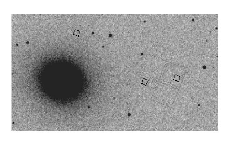
Figure 1: Locations of the three NIC-2 fields (smaller dark squares) in the halo of NGC3379. At distances of 3′, 4.5′, and 6′from the nucleus, these fields have mean B surface brightnesses of 25.2, 26.4, and 27.2, respectively. The outermost field is contained within the WFPC2 field of Sakai et al. (1996), also indicated.

Observations of each of the three fields were divided evenly between two epochs, spaced 2-3 months apart to identify candidate variable stars. The interval was set by HST scheduling constraints and the desire to have the same orient for follow-up visits, while obtaining all data in a single observing cycle. A drawback in observing at two epochs was the significant increase in zodiacal light during the second visits. The overall background was roughly twice as high, completely consistent with the variation in zodiacal light due to the object-HST-Sun viewing angle changing from $\sim 145\arcdeg$ to $\sim 56\arcdeg$.

Data were taken using $\sim 1400$s MULTIACCUM SPARS64 integration sequences; the fields were dithered by a few pixels between sequences. The total integration time spent in each filter for each field is 11.2 ksec (8 MULTIACCUM sequences). We initially planned to divide the exposure times between $F160W$ and $F110W$ with a 5:3 ratio. After the first epoch observations, however, it was evident that we were not obtaining sufficient depth in $F110W$, so the second visits were used to equalize the total exposure times in the two filters.

Table 1: NICMOS Observing Log 1998

Field 1 (93 day interval)			Field 2 (62 day interval)			Field 3 (63 day interval)
Epoch	Filter	Int. time	Epoch	Filter	Int. time	Epoch	Filter	Int. time
Apr 02	$F160W$	1343.9	May 02	$F160W$	1343.9	May 03	$F160W$	1343.9
		1407.9			1407.9			1407.9
		1407.9			1407.9			1407.9 SAA
		1407.9			1407.9			1407.9
		1407.9			1407.9			1407.9 SAA
	$F110W$	1407.9		$F110W$	1407.9		$F110W$	1407.9
		1407.9			1407.9			1407.9
		1407.9			1407.9			1407.9 SAA
Jul 04	$F160W$	1407.9	Jul 03	$F160W$	1407.9	Jul 05	$F160W$	1407.9
		1407.9			1407.9 saa			1407.9 SAA
		1407.9			1407.9 SAA			1407.9 saa
	$F110W$	1343.9		$F110W$	1343.9		$F110W$	1343.9
		1407.9			1407.9			1407.9
		1407.9			1407.9			1407.9
		1407.9			1407.9			1407.9 saa
		1407.9			1407.9 SAA			1407.9 SAA

Note. — “SAA” means the data were judged too badly affected by SAA CR persistence to be useful; “saa” means that the data show signs of CR persistence, but are still included in the final images.

Only the innermost field is uncompromised by cosmic ray (CR) persistence during South Atlantic Anomaly (SAA) passage. Severely affected data were omitted from the final images, resulting in reduced total exposure times. The combination of higher background and CR persistence has rendered the second epoch $F160W$ images for Field 2 nearly useless. The outer field which overlaps with the previous WFPC2 data is also seriously impacted, with effective exposures of only 6975s in $F160W$ and 8383s in $F110W$, and even these have noticeable CR persistence. A log of the observations is given in Table 1.

3 Data Reduction

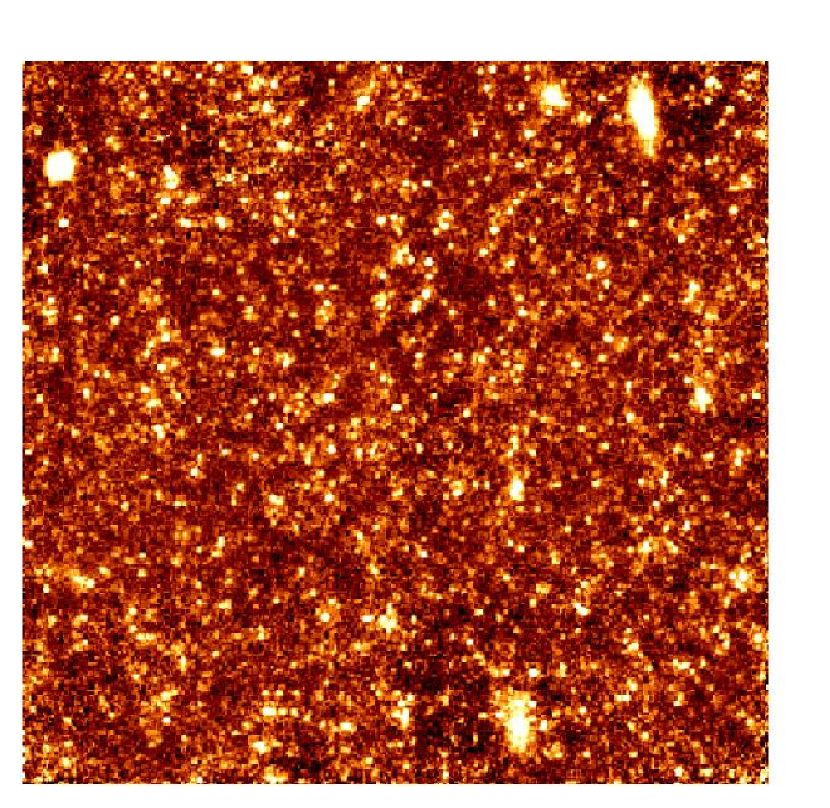
Figure 2: Final drizzled, combined $F160W$ (H band) image of the innermost field in the halo of NGC3379, 3′ from the nucleus. Total integration time is 11.2ks. These data were little affected by SAA passages. One bright Galactic foreground star is present in the upper left corner.

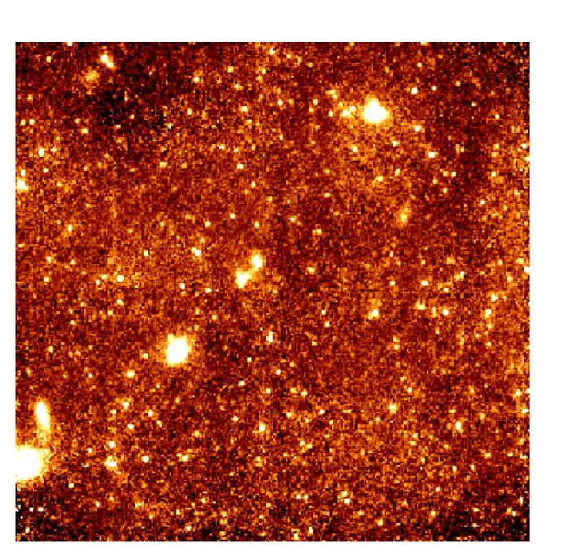
Figure 3: Final drizzled, combined $F160W$ (H band) image of the middle field in the halo of NGC3379, 4.5′from the nucleus. The total exposure time is 9.8ks; one MULTIACCUM sequence being badly affected by SAA passage. A number of extended background sources contaminate the field.

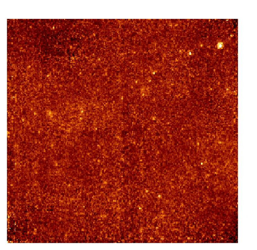
Figure 4: Final drizzled, combined $F160W$ (H band) image of the outermost field in the halo of NGC3379, 6′from the nucleus. The total exposure time is 7.0ks; several MULTIACCUM sequences being badly affected by SAA passage. One bright Galactic foreground star is present in the upper right corner.

The raw NICMOS images were reduced using IRAF scripts kindly provided by M. Dickinson (1998, private comm.) These scripts are very similar to the now-public versions released in mid-1999 which improve on the original CALNICA pipeline procedures, primarily in the removal of the quadrant-dependent bias level or “pedestal” signature. Updated dark frames which included the modeled temperature dependent variable bias level (“shading”) correction were supplied by E. Bergeron. A correction was also made to remove excess shot noise from non-optimum dark subtraction; this was done by subtracting a noise-free map of the difference between the non-optimal pipeline dark correction and a more accurate, very deep blank field frame; this “delta-dark” was also supplied by M. Dickinson.

The 8 reprocessed individual MULTIACCUM exposures in each filter were then registered using xregister in IRAF. At this point it was possible to assess the impact of the SAA on individual exposures. The unaffected MULTIACCUMs were then combined using the “drizzle” technique (Fruchter & Hook 2002) to produce images subsampled by a factor of 2 using a 0.9 drop size. A very low order smooth surface was fit to the individual frames and subtracted to remove the background to bring all the frames to the same mean value, necessary to achieve good results when drizzling. A mean sky level was added back to the final frame to preserve background counts for computing photometric errors. To look for variable stars, separate images were made for each of the two epochs in the same manner.

The final drizzled $F160W$ images are shown in Figure 2-4. The substantial gradient in stellar density from field to field is immediately apparent. A string of background galaxies is visible in the middle field. The outermost field is of very limited value because it is so sparsely populated with stars, partly because of its extreme outer location but also because it is most impacted by the higher noise levels and reduced effective exposure times due to SAA CR persistence. This is quite unfortunate because this field overlaps with the previous WFPC2 $I$-band observations. This NICMOS location detects so few stars, in fact, that comparison with the optical data is useless.

4 Photometry

4.1 PSF Fitting and Calibration

Point-spread-function (PSF) fitting photometry was performed using standard iraf/daophot procedures, after masking out obvious background galaxies and the NICMOS coronograph hole. Attempts to construct a reliable PSF model from the data were not successful primarily because crowding raised the noise level in the wings of the bright, well-exposed stars to unworkable levels. Instead, we used the tiny tim package (Krist 1993) to construct NICMOS $F110W$ and $F160W$ PSFs. We added “jitter” to the tiny tim models until we reproduced the well-determined cores of the empirical PSFs in the final drizzled images. Because of the better-behaved profile wings, the model PSFs gave much better results when used in the daophot routines, judging from the lower residuals in the subtracted images and the much lower photometric errors.

We used apertures of 2.5 ($F110W$) and 3.0 ($F160W$) pixels radius to measure the instrumental magnitudes in each drizzled image. Objects were found independently in $F110W$ and $F160W$ and then matched with a cutoff distance of two drizzled pixels, allowing for possible small registration errors, geometric distortions, and noise. Using modeled PSFs for the photometry made determination of the aperture corrections straightforward; from the measurement aperture to a 0$\farcs$5 radius (13.33 drizzled pixels) required an $F110W$ correction of $-0.65$ magnitudes while the $F160W$ correction is $-0.78$. These magnitudes were then corrected to “infinite” apertures with the standard factor of 1.15. We adopted the NICMOS Data Handbook “Vega magnitude” zeropoints of 1775.0 mJy in $F110W$ and 1040.7 mJy in $F160W$. The photometry has also been corrected for the small Galactic extinction towards NGC3379, 0.022 and 0.014 magnitudes in $J$ and $H$ (Schlegel, Finkbeiner, & Davis 1998).

To ensure that only the best measured stars are used in the analysis, the photometry was then filtered against several criteria reported by the PSF fitting task. Objects with $\chi^{2}>2.5$, “sharpness” parameter outside the range $-0.9$ to $1.$, and photometric error $>0.5$ in $F110W-F160W$ were discarded. The first two criteria eliminate nearly all extended objects, residual bad pixels, and edge effects. Total numbers of objects with both $F110W$ and $F160W$ photometry meeting the above criteria are 1751, 477, and 144 in Fields 1, 2, and 3, respectively. The statistics of the photometric errors are reported in Table 2.

Table 2: Photometry Statistics

$F160W$			$F110W-F160W$
Mag	$<Error>$		Mean	$<Error>$	RMS
22.50	0.020		1.350	0.032	0.22
23.00	0.024		1.436	0.048	0.21
23.50	0.033		1.362	0.056	0.21
24.00	0.048		1.358	0.080	0.24
24.50	0.072		1.275	0.111	0.30
25.00	0.107		1.174	0.161	0.43

Note. — The RGB tip is at $F160W=23.68$.

4.2 Identification of Variable Star Candidates

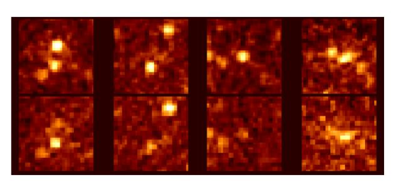
Figure 5: Four examples of variable star candidates from the inner $F160W$ field are displayed with the brighter epoch above. The first pair is the most significant variable in the images with $\Delta F160W>1.1$, fading from $22.9$ to $24.0$ during the 3 month interval between observations. Both of the bright stars in the second pair of images are identified as variable. The rightmost is a fainter example, with $<F160W>=24.1$ and an amplitude of 0.6 magnitudes.

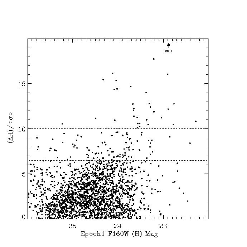
Figure 6: Variable star identification was done by comparing the change in magnitude between epochs relative to the photometric errors for every object identified in both epochs of $F160W$ images. Because stars may vary below the detection threshold in one epoch, this approach may miss some of the most extreme variables, but all stars with $F160W<24$ were recovered in both epochs. The variable with the highest significance is off the top of the plot (arrow).

Table 3: Field 1 Variable Star Statistics

F160W range	NTOT	NVAR	FVAR
$22.2-23.65$	0098	38	0.388
$23.65-24.0$	0197	24	0.122
$24.0-24.5$	0503	33	0.066
$24.5-25.0$	0569	29	0.051
$25.0-25.5$	0329	02	0.006
$22.2-25.5$	1696	121	0.071

Note. — The RGB tip is at $F160W=23.68$

The observations were split between two epochs for the express purpose of detecting variable stars. The intervals for fields 1, 2, and 3, are 93, 62, and 63 days, respectively. Blinking the reduced images immediately revealed many variables (Figure 5). To quantitatively identify and characterize the variable star candidates, we separately ran daophot on the reduced and combined images for each epoch. The positions of stars determined in the total integration time images were used to constrain the photometry for the noisier separate epoch images. With just two epochs, the problem of identifying variable star candidates reduces to gauging the significance of the change in brightness of a star from first to second epoch, which can be done in myriad ways. For Field 1, we show $\Delta(H)=(F160W_{1}-F160W_{2})$ divided by the photometric errors summed in quadrature from each epoch, plotted against the first epoch $H$ magnitude (Figure 6). Because stars may vary below the detection threshold in one epoch, some of the most extreme variables are potentially missed, but, as it happens, all of the stars in the combined image brighter than $F160W\approx 24$ were detected in both epochs.

The dotted lines at the 6.5 and 10 “sigma” levels are drawn to help evaluate the diagram, but can also be taken as liberal and conservative criteria for variability. In Field 2, no variables were reliably detected because the second epoch images are so shallow due to SAA problems. A few stars qualified as variable in Field 3.

Many of the brightest stars with the tiniest photometric errors are among the most significantly variable (Figures 5, 6), providing confidence that the majority of the brightest stars are not due to crowding of ordinary red giants. The fractions of variables as a function of $F160W$ magnitude are listed in Table 3.

5 Luminosity Functions

The $F160W$ luminosity function (LF) histograms for the combined epoch imaging data for Fields 1 and 2 are shown in Figure 7; bin size is 0.1 magnitudes. Field 3 has such poor statistics – no stars at all within 0.25 magnitudes of what will turn out to be the RGB tip – that we will not discuss its LF further. The Field 1 and 2 distributions both begin to turn over in the $F160W=24.7$ bin, suggesting that this is where incompleteness becomes important. This is confirmed by the artificial star tests which indicate $\sim 80\%$ completeness at this brightness (see Appendix A). The LF for Field 1 (shown with and without the variable candidates) shows a definite jump in the number of stars in the bin spanning $23.65-23.75$, which we attribute to the brightness limit of the helium-burning RGB tip. Omitting the variables, nearly all of which are probably AGB rather than RGB stars (see $\S$6.1.4), increases the significance of this break in the luminosity function; the RGB tip bin has more than 2.5 times as many non-variables as the next brighter bin.

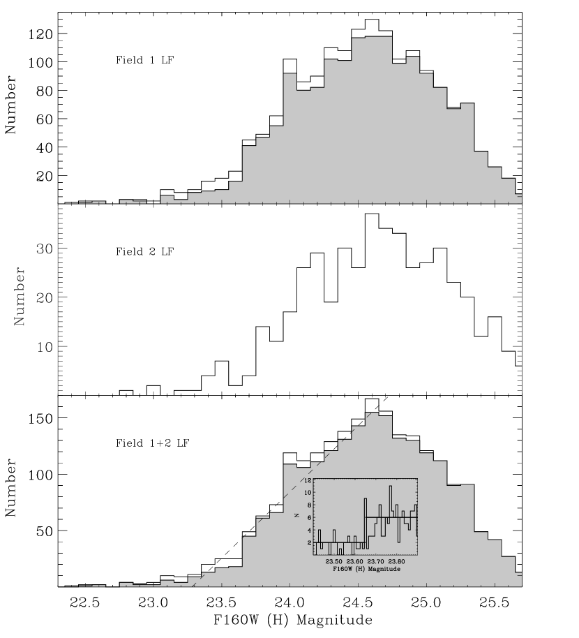
Figure 7: The luminosity functions of the two inner NICMOS fields, and their sum. The unshaded portions of the upper and lower panel histograms show the contribution from variable star candidates. The clear break at $F160W=23.65$ is due to the tip of the RGB; a higher resolution close-up of this region is displayed in the lower panel. Maximum-likelihood fitting yields a best-fit TRGB magnitude of 23.68. The feature at $F160W=24.0$, either an excess or a change in slope, may be due to an AGB star contribution. The dashed line is a robust linear fit to the nonvariable star bins with $23.65\leq F160W\leq 24.6$

The Field 2 distribution shows a similar but not as prominent break in the next fainter bin, $23.75-23.85$ magnitudes. As both fields are at the same distance, this shift, if real, could indicate a modest metallicity difference of $\sim 0.1$ dex (see $\S 6$), but with the small number of stars in Field 2, this is not highly significant. The summed LF is shown in the bottom panel; the two histograms again being with and without the variables from Field 1. In the combined LF, the significance of the RGB tip break remains roughly the same as for Field 1 alone (2.50 times as many nonvariable stars as the next brighter bin), even though we are unable to flag variables in Field 2. The slope of the LF is close to linear over the brightest magnitude of the RGB, as shown by the dashed line fit to the nonvariables in Figure 7. This fit predicts that the first bin brighter than the RGB tip should contain more than twice as many stars as observed (37 vs. 18).

5.1 Pinpointing the Magnitude of the Tip of the RGB

A blow-up histogram of the break region is shown in the inset; the bin size is reduced to 0.01 magnitudes. Even at this fine scale, there is an obvious increase in the numbers of stars in each bin beginning at $F160W=23.65$. In the inset, the median number of stars per bin brighter than this is 2; fainter is 6, firmly placing the RGB tip magnitude at a level where the formal photometric errors are only $\pm 0.04$ magnitudes per star. There are about a dozen stars within 0.01 magnitudes of the tip of the RGB, so the error budget for the RGB tip magnitude is dominated by the systematic uncertainty in the photometric calibration of NICMOS – $5\%$ – over any other source of error. Artificial star tests show that crowding effects for Field 1 introduce a median systematic error of only $\sim 0.01$ magnitudes per star at this brightness (Appendix A). In the face of 0.04 magnitude errors, the extremely sharp break at $F160W=23.65\pm 0.01$ must be partly fortuitous, but certainly suggests an unambiguous placement of the RGB tip. To obtain a completely objective estimate of the RGB tip apparent magnitude, we employed a maximum likelihood approach. Figure 8 shows the composite field 1+2 luminosity function (excluding the identified variable stars) on a logarithmic scale with 0.04 magnitude binning. We have determined the magnitude of the TRGB by fitting a two power-law model:

$$N(f)=\left\{\begin{array}[]{ll}f^{\gamma_{1}}&\mbox{for $f>f({\rm TRGB})$};\\ Af^{\gamma_{2}}&\mbox{for $f<f({\rm TRGB})$}.\end{array}\right.$$

The free parameters are $f({\rm TRGB})$, the flux corresponding to the TRGB magnitude, the amplitude of the TRGB discontinuity, $A$, and the two power-law indices $\gamma_{1}$ and $\gamma_{2}$. To constrain the models, we perform a maximum-likelihood fit on the unbinned magnitudes. As a simplification in our maximum-likelihood fit, we have not convolved the model with the magnitude errors. At the TRGB the median error is 0.035 mag. We verify through Monte-Carlo simulations that this simplification does not significantly bias the results (see below). For each set of model parameters we compute the probability distribution of star fluxes. We then vary the parameters of the model, maximizing the log of the likelihood of observing the data. Fitting data in the range $22.5<F160W<24.5$ (905 stars) we find a best-fit TRGB magnitude of F160W = 23.68. The best-fit model is shown as a solid line in Figure 8.

Figure 8: The composite LF of Fields 1 and 2 (excluding the identified variable stars) on a logarithmic scale with 0.04 magnitude binning. The unbinned data for the 905 stars in the range $22.5<F160W<24.5$ are modeled with two power laws using a maximum-likelihood fit. The best-fit model (solid line) yields a TRGB magnitude $F160W=23.68$ with 68% confidence interval of $23.63<F160W<23.70$.

We have assessed uncertainties in two ways: (1) by bootstrap resampling the data and re-performing the fit and (2) by creating simulated data sets with realistic magnitude errors and known LFs and carrying maximum-likelihood fits to verify that the input parameters can be recovered. The 68% confidence interval spans the range $23.63<F160W<23.70$ and the 95% confidence interval is $23.62<F160W<23.76$. The parameters $\gamma_{1}$ and $\gamma_{2}$ have been allowed to vary in these experiments — the best-fit TRGB magnitude is remarkably robust.

The Monte-Carlo simulations allow us to determine if the fitting procedure introduces any bias. In our simulations, data points are drawn from a model distribution function and scattered with a magnitude-dependent error derived from the real data data: $\sigma(m)=10^{0.03449m-9.605}.$ Ten thousand data sets with the same number of data points as the observed sample are created and best-fit model parameters determined using the identical maximum-likelihood procedure that was applied to the real data. We tried input models with a range of parameters similar to the true data. As a typical example, for a model with parameters $m({\rm TRGB})=23.65,A=2.0,\gamma_{1}=-2.3$ and $\gamma_{2}=-4.3$, we recover in 10000 Monte-Carlo iterations $m({\rm TRGB})=23.64\pm 0.02.$ Ignoring the magnitude errors in performing the maximum-likelihood fits thus does not appear to introduce any significant bias in the results. The dominant source of error in the RGB tip magnitude is likely to be the 5% systematic uncertainty in the NICMOS photometric calibration. Departure of the true shape of the LF relative our the simple model of a sharp discontinuity — due to binaries, stellar rotation, variability, and the finite metallicity spread, for example — is another possible source of systematic error for the TRGB-distance technique.

While in principle the LF in $F110W$ might provide additional information on the TRGB location, the tip is much less pronounced in $F110W$. In $\S 6$, it will be shown that NGC3379 has a large abundance spread. Theoretical isochrones show that the TRGB is a strong function of abundance in the $F160W$ band, with the solar and near-solar metallicity TRGBs rising well above the more metal-poor TRGBs, effectively producing a nearly single-abundance TRGB to measure. In $F110W$, however, the RGB tips of different metallicity populations are closer together in luminosity, and the large abundance spread of NGC3379 blurs the discontinuity so evident at $F160W=23.68$ (Figure 7).

5.2 Other Luminosity Function Details

In Field 1, there are 98 stars in the bins brighter than the tip; 38 of these (39%) are variable candidates. These will be discussed further in the next section, along with the implications for the distance and stellar population of NGC3379. Also in Field 1, there is an excess of stars in the bin centered at $F160W=24$, which, in the summed LF becomes another apparent break: the LF jumps by a factor of 1.65, then falls again. This excess is not as statistically significant as the brighter RGB tip break, and occurs in just one or two bins. Taking the average number of nonvariables in the bins on either side of this feature predicts 85 stars whereas 109 are seen, about a $2.5\sigma$ difference. This second break can be interpreted as an AGB contribution and is discussed further in $\S 6.1.4$.

6 Color Magnitude Diagrams

The NICMOS CMDs for each of the three fields are compared in Figure 9. The variable star candidates identified in Figure 6 from Fields 1 and 3 are circled, double circles indicating the variables with significance levels $>10$. The colored solid lines trace the smoothed, running median color ridge lines, with the dotted lines indicating one standard deviation; the ridges are computed using stars with $F110W-F160W\leq 2.0$ only. Objects with redder colors, especially faint objects, are probably galaxies, consistent with the roughly constant numbers of such objects from field to field. For reference, the horizontal dotted lines mark the location of the RGB tip found from analysis of the LF histograms ($\S 5.1$, Figure 7).

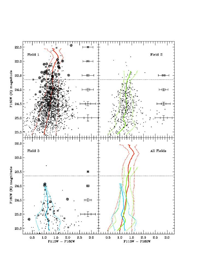
Figure 9: Comparison of the color-magnitude diagrams of the three NICMOS fields in NGC3379. Circled stars have varied by 6.5 or 10 sigma (single and double circles, respectively; the second epoch data for field 2 are not deep enough to confidently identify variables). The mean (solid) and one standard deviation (dotted) ridge lines of each field are shown and reproduced together for comparison in the lower right panel; objects with colors $>2.0$ are probably background galaxies and have been clipped from the ridge line determinations. There is no significant difference in the three populations spanning nuclear distances of 9 kpc to 18 kpc. The horizontal dotted line marks the magnitude of the TRGB. The sloping dashed line indicates the 50% completeness level for Field 1; confusion of the unresolved stellar background is a greater limitation.

NGC3379 is at Galactic coordinates $l=133^{\circ},b=57^{\circ}$. There are two obvious bright foreground stars in the images, one each in Fields 1 and 3 (Figures 2 and 4). Scaling from star counts in the Hubble Deep Field (Williams et al. 1996; Méndez & Minniti 1999) and infrared Subaru Deep Field (Maihara et al. 2001), we estimate that over the magnitude range displayed in Figure 9, $22.3<F160W<25.7$, the expected number of Galactic foreground stars is zero.

Two sets of $F110W-F160W$ error bars are shown: the inner are the median $F160W$ photometric errors reported by daophot, determined in half-magnitude bins. The outer error bars show the $1\sigma$ widths of the $F110W-F160W$ color distribution at each magnitude level, again determined in half-magnitude intervals. The bright limits of the ridge lines are determined solely by the extent of the data and are not meant to suggest the locations of the RGB tip or any other stellar evolutionary phase. The three ridge and dispersion lines are over-plotted for comparison in the lower right panel of Figure 9. There is no significant shift of the main RGB locus from one field to another, and, given the small number of stars in Field 3 and the similarity of the loci for Fields 1 and 2, these data suggest that there are no substantial differences in the stellar populations of the three fields. Most of our subsequent analysis is based on Field 1 alone, but by implication applies to the other fields as well.

6.1 Comparison to Theoretical Isochrones

Determination of the metallicity and spread in abundance of the stars in NGC3379 was a primary motivation of this project. Using the best-fit RGB tip magnitude of $F160W=23.68$ found above, it is possible to derive a distance to NGC3379, in turn allowing constraints on its age and metallicity by comparing the NICMOS CMDs to theoretical isochrones. We have considered two independent sets of isochrones: the latest version of the Bruzual & Charlot (1993) models (BC; see also Liu, Charlot & Graham 2000), kindly provided in advance of publication by S. Charlot, plus the isochrones of Girardi et al. (2002). The BC isochrones are derived largely from the “Geneva” evolutionary tracks (Maeder & Meynet 1989) while the Girardi set is based on the “Padova” evolutionary tracks (Bertelli et al. 1994).

6.1.1 Mean Metallicity and Age Constraints

In Figure 10, upper RGB isochrones for 3, 5, 8, 10 and 15 (or 14) Gyr populations with [Fe/H]=$-0.7$, 0.0, and $+0.4$ or $+0.2$ are over-plotted on the ridge lines for Field 1. Also plotted are the standard deviation lines (dashed) of the observed NGC3379 giant branch. The isochrones have been shifted to match the observed RGB tip magnitude, $F160W=23.68$, in NGC3379. The resulting individual distance moduli are listed in the figure. For the Girardi isochrones, the AGB loci are also plotted (dotted lines). The AGB in the BC isochrones do not rise more than a few hundredths of a magnitude above the RGB tip.

Both sets of isochrones demonstrate that the location of the RGB in an infrared CMD depends primarily on metallicity while age is a second order effect. Neither set of [Fe/H]=$-0.7$ isochrones for any age reproduces the mean color location of the RGB in NGC3379; the data demand a much higher abundance. The younger super-solar isochrones are perhaps a reasonable match in principle, but the relatively bright and blue turnoff of a majority 3-5 Gyr population would be incompatible with the optical broad band colors and spectrophotometry of NGC3379 (Terlevich & Forbes 2002), although strictly, the integrated light analysis applies only to the nuclear regions. This leaves open the somewhat unlikely possibility that the halo comprises mainly very metal rich intermediate age stars. Additional age constraints based on the CMD come from consideration of the observed AGB, which is better fit by the older ($>8$ Gyr) isochrones of Girardi et al. (2002), as will be shown in $\S 6.1.4$.

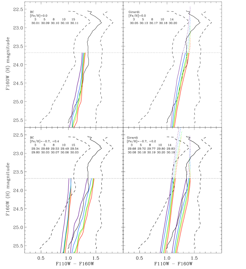
Figure 10: Comparison of isochrone ages and abundances. All isochrones have been shifted so that their RGB tips are at $F160W=23.68$, out best-fit tip magnitude; the corresponding distance moduli in each case are listed. Both the BC and the Girardi isochrones indicate a roughly solar mean abundance and a mean age of 10 to 15 Gyr. The dotted colored lines show the loci of the upper AGB in the Girardi isochrones.

The solar abundance, 8, 10 and 14/15 Gyr isochrones of either set bracket the RGB ridge line down to $F160W=25$. At this magnitude, the observed RGB begins to get bluer. The blueward trend is from incompleteness in the $F110W$ band and the onset of confusion close to the limit of the data (Appendix A). The brightest 0.5 magnitude of the RGB of the solar BC isochrones do not track the observed ridge line as well as the corresponding Girardi isochrones.

The isochrones thus constrain the mean abundance of NGC3379 to be close to solar metallicity, independent of the age of the stellar population. While the usual age-metallicity degeneracy still affects the conclusions at some level, the mean age is likely to be in the range $8-15$ Gyr, probably very close to 10 Gyr. Given the relatively small offsets in color due to age in the $F110W-F160W$ colors, and the relatively large observed width of the RGB, a considerable spread in age above $\sim 8$ Gyr cannot be ruled out.

A metallicity close to solar is perhaps surprising so far out in the halo, even of a giant elliptical. One possible explanation for the high abundance is that NICMOS is measuring the brightest, most metal rich stars. Looking at the CMDs and isochrones in Figures 9 and 11, the metal poor populations are fainter and bluer. Stars with [Fe/H]$<-1.7$ will drop below the sensitivity range of the observations. The mean abundance of the measured stars is close to solar, but a deeper census might reveal the existence of a bluer, much lower abundance population with [Fe/H]$<-2$. This effect is the opposite of what happens in the optical where $V$ (and even $I$) band RGBs become fainter with increasing metallicity, leaving just the metal poor stars to be measured in shallow observations, resulting in a lower mean abundance. With the present NICMOS data we may be overestimating the mean metallicity. Complementary deep $V$ and $I$ band observations with the Advanced Camera for Surveys (ACS), especially leveraged against these and/or additional NICMOS fields, are required to document the full extent of the metallicity spread in NGC3379.

6.1.2 An Infrared RGB Tip Distance to NGC3379

The sharpness of the break in the LF and the small photometric errors at the RGB tip ($\pm 0.035$ magnitudes per star), provide a robust location of the RGB tip from the maximum-likelihood analysis. Adopting the solar metallicity, 10 Gyr isochrone as the best fit, the implied distance modulus to NGC3379 is 30.10 (10.4 Mpc) for the BC isochrone, $+0.08$ greater for the Girardi isochrone. The major contributors to the uncertainty in distance are the NICMOS photometric calibration and the isochrone differences. The NICMOS absolute calibration is good to $\pm 0.05$ magnitudes according to the NICMOS website. The Girardi et al. isochrones are systematically brighter and redder than those of BC, the solar 10 Gyr RGB tip in particular by 0.08 magnitudes. Much of this difference could arise from the coarseness of the isochrone sampling of the RGB in steps of $\sim 0.05-0.07$ magnitudes. Both the NICMOS calibration and the isochrone differences are systematic in nature and we conservatively add them linearly to derive a total uncertainty. The total error in the distance estimate is $\pm 0.14$ magnitudes, only 7% in distance, almost entirely from the uncertainties due to systematic differences between the theoretical isochrones and the NICMOS absolute photometric calibration, not the data.

Averaging of the two isochrone sets leads to $m-M=30.14\pm 0.14$ (10.67 Mpc $\pm 0.74$) as the distance for NGC3379. Our estimated $1\sigma$ error includes the full covariance of the TRGB magnitude with respect to the other parameters in the model, but does not include possible systematic effects due to the abundance spread, which we have not included in the maximum-likelihood analysis in $\S 5.1$. The mean abundance of NGC3379 is very near solar, and, fortuitously, the solar abundance isochrones of either BC or Girardi et al. (2002) have the most luminous (or nearly the most luminous) TRGB, so modest contributions of stars from non-solar abundance populations will not significantly affect the detection of the brightest (roughly solar abundance) TRGB location.

The better match of the upper RGB and the better representation of the brighter AGB stars by the Girardi isochrones supports a preference for an increase in the distance to $m-M=30.18$ (10.86 Mpc); a positive choice of one set of isochrones over the other also removes a contribution of 0.08 magnitudes to the systematic errors, which would reduce the error estimate to $<0.1$ magnitudes. Regardless, the derived distance is in good agreement with estimates by other techniques (Gregg 1997; Hjorth & Tanvir 1997), and consistent at the $1\sigma$ with the results of Sakai et al. (1997) who found $m-M=30.30\pm 0.14$ (random errors) $\pm 0.23$ (systematic) from the $I$-band luminosity of the RGB tip using WFPC2 imaging.

6.1.3 Metallicity Spread

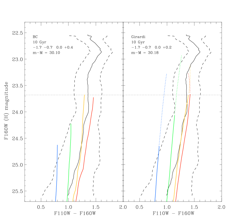
Figure 11: The 10 Gyr isochrones of various metallicities, all shifted to the same distance modulus (30.10 for the BC isochrones, 30.18 for the Girardi), compared to the mean color-magnitude distribution (solid black line) of NGC3379. The observed RGB tip magnitude is indicated by the horizontal dotted line. The dotted colored lines show the upper AGB loci of the Girardi isochrones. The one standard deviation dashed ridge lines are consistent with the presence of stars with the wide range of metallicities shown.

The metal poor isochrones are not a good match to the mean RGB of NGC3379, but provide constraints on the metallicity spread. From examining the isochrone sets in Figure 10, it is clear that it is impossible to account for the RGB width solely with an age spread; most or all of the intrinsic width must be due to a spread in abundance. In Figure 11, over-plotted on the Field 1 ridge and dispersion lines are BC and Girardi 10 Gyr isochrones for a range of abundance, all shifted to the same distance modulus, 30.10 for BC and 30.18 for Girardi. In both isochrone sets, the lower abundance RGB tips have lower luminosity and are shifted to bluer colors, naturally tracing the blue envelope of the observed RGB stars. A range of metallicity will thus increase the intrinsic (and observed) width of the RGB at fainter magnitudes, even without a contribution from increasing photometric errors, because there simply are no extremely metal-poor RGB stars brighter than $F160W\approx 24.5$. The super-solar BC isochrone also has a somewhat fainter RGB tip luminosity, perhaps signaling the same effect on the high metallicity side.

Consequently, the isochrones predict that for a heterogeneous abundance stellar population, the spread in metallicity will be a function of magnitude over the upper $\sim 1.5$ magnitudes of the RGB. The color distributions in four 0.5 magnitude intervals beginning at the RGB tip are plotted in Figure 12. Over-plotted on each is a best-fit gaussian with the same standard deviation and median, normalized to the total number of stars. The upper abscissa is an approximate metallicity scale computed simply by dividing the isochrone metallicity range (2.1 dex) by the color difference at the central $F160W$ in each interval. This is approximate and plotted merely for reference; the change in color is not strictly a linear function of abundance, nor constant as one goes down the RGB.

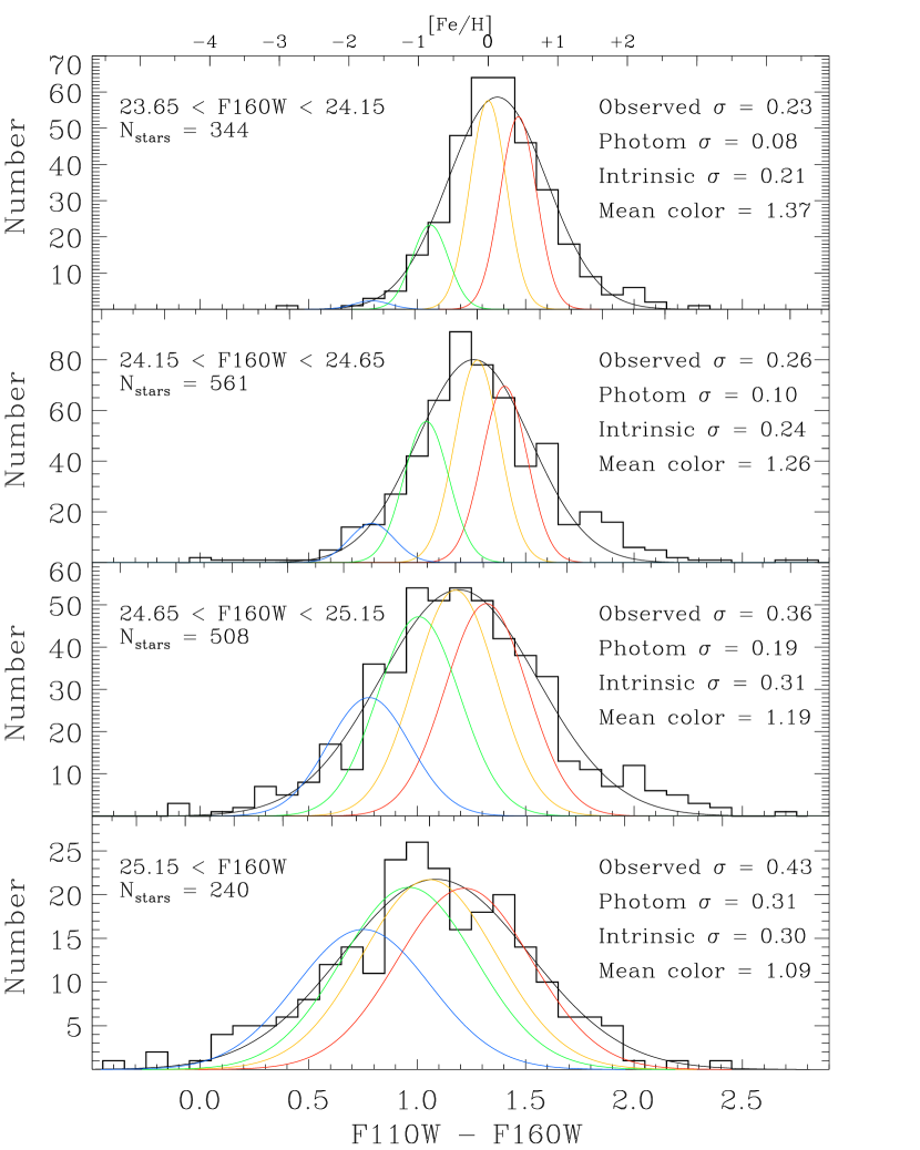
Figure 12: Observed color spread of the RGB (histograms) in four magnitude intervals compared to the widths expected from photometric errors alone, as determined from artificial star tests. The broad gaussian in each panel is a robust fit to each histogram; the narrower histograms show the expected widths and locations for hypothetical single abundance populations with the metallicities shown in Figure 10, their peaks scaled to fit on the broad gaussian. These qualitatively show the relative contributions of each abundance interval, mainly illustrating the increasing contribution of the metal poor stars at fainter magnitudes. We have used the BC isochrones for this analysis because of their higher maximum Z.

For comparison, we also plot gaussians at the mean color location of the 10 Gyr BC isochrones with [Fe/H] = $-1.7,-0.7,0.0,+0.4$. Each has a $1\sigma$ width equal to the spread in color caused by crowding and photometric errors, as determined by our artificial star tests (Appendix A). The peaks are simply scaled to the local value of the total gaussian fit and so these are meant to be suggestive only; the abundance distribution of the stellar population is, as far as we can tell from our data, continuous. The near absence of any contribution from extremely metal-poor blue stars in the brightest interval is evident, as discussed above. Such blue stars become numerous at magnitudes $>24.5$, once the tip of the fainter metal-poor RGB enters the plots. The presence of stars redder than the [Fe/H]$=+0.4$ isochrone implies a very metal-rich population. The intrinsic width of the color distributions increases gradually from 0.21 to 0.31 magnitudes over the three brightest intervals, but does not increase further in the faintest, suggesting that we may be seeing the full extent of the abundance spread, but deeper data are required to confirm this. The faintest interval is essentially confusion limited (see Appendix A), however, so while it is consistent with the next brighter interval, it cannot bear much weight in the analysis.

Using the color-to-metallicity conversions computed from the isochrones, the metallicity spreads in each 0.5 magnitude interval on the RGB are $\pm 0.6$, $\pm 0.8$, $\pm 1.2$, and $\pm 1.2$ dex. The tail to very red objects, $F110W-F160W\gtrsim 2.$ is perhaps due to unresolved galaxies. There is a suggestion of a break in the middle two color histograms at $F110W-F160W\approx 1.65$, perhaps an indication of the transition between the stellar population and the background galaxies. The blueward trend of the most metal-rich isochrones with fainter magnitudes combined with photometric errors may produce this break on the red side. Extrapolating from the BC isochrones, we estimate that this color corresponds to [Fe/H]$\approx+0.8$. Stars this metal-rich have been shown to exist in the inner Milky Way halo (Rich 1986; Minniti et al. 1995; Sadler, Rich, & Terndrup 1996), coexisting with extremely metal poor objects of $[Fe/H]=-2$ (Blanco 1984), similar to the situation we find in NGC3379.

6.1.4 The Asymptotic Giant Branch Population

The characteristics of the AGB population evolve with age and are a function of metallicity, so in principle the AGB can be a stellar populations diagnostic. To be useful, though, the AGB contribution must somehow be separated from the RGB, which is problematic when photometric errors and stellar physics cause them to completely overlap fainter than the RGB tip.

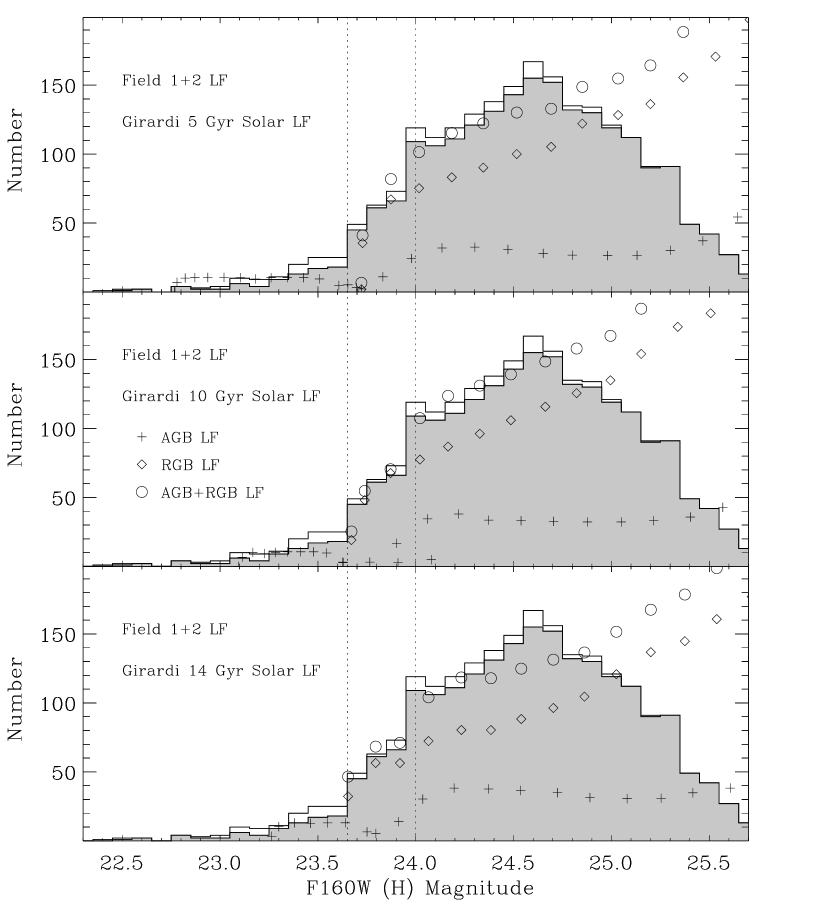
Figure 13: Theoretical luminosity functions (points) based on the Girardi solar metallicity isochrones were computed using a Salpeter initial mass function (x = 1.35) for comparison to the observed LF, with and without variables (histograms), of NGC3379. The 10 and 14 Gyr models, or a composite, can account for the majority of AGB stars above the RGB tip. The break in the observed LF at $F160W=24.0$ is qualitatively accounted for by a decline in the brighter AGB population.

Stars significantly brighter than the RGB tip, however, can be relatively easy to isolate; work by Mould & Aaronson (1979) showed that such AGB stars mark the presence of intermediate age populations, $\lesssim 3$ Gyr. Yet the existence of stars up to $\sim 1$ magnitude brighter than the RGB tip in metal rich Galactic globular clusters (Guarnieri, Renzini, & Ortolani 1997), advises caution in interpreting such stars as an unambiguous signal of younger populations. The behavior of the AGB in the Girardi isochrones (Figures 10, 11) also shows that stars brighter than the RGB tip by up to $\sim 1$ magnitude can be expected even in ancient populations. We find 98 stars above the tip of the RGB in Field 1 (Table 3, Figure 9), 38% of which are variable, and an additional 19 bright stars in Field 2, plus one more in Field 3. All but 13 of these are within 0.6 magnitudes of the RGB tip.

To test the conclusions from $\S 6.1.1$ that the population of NGC3379 is old and solar metallicity, we computed theoretical LFs using a Salpeter initial mass function (IMF) using the Girardi 5, 10, and 14 Gyr solar isochrones. The resulting comparison with the observed $F160W$ LF is necessarily approximate as the isochrones are sampled in uneven mass bins determined by theoretical considerations while the observed LF has been computed in equal magnitude bins. We have not interpolated the isochrones because this smooths out sharp features such as the RGB tip and also because the isochrones are not monotonic functions in luminosity in regions of interest, making interpolation problematic. Fortuitously, the isochrone mass intervals correspond to magnitude intervals of 0.1 to 0.15 along the RGB. We have, however, rebinned the theoretical AGB LF to the same magnitude intervals as the theoretical RGB to permit easy summing and have scaled the total LFs by eye to give an approximate match to the observed LF (Figure 13).

The 10 or 14 Gyr isochrones, or a composite, can account for the AGB stars up to 0.6 magnitudes brighter than the RGB tip. These stars then do not require an intermediate age or younger population in NGC3379. Any claim of such a population would rest on the 13 yet brighter AGB stars ($F160W<23.0$). Such stars are predicted by the 5 Gyr isochrone, but the numbers of observed AGB stars above the TRGB limit any 5 Gyr contribution to $\sim 20\%$ of the total. The brightest AGB stars are more naturally explained by a contribution from the substantial [Fe/H]$=-0.7$ component needed to account for the metallicity spread (c.f. Figure 11); this population will generate AGB stars up to 0.8 magnitudes above the RGB tip. Blends of stars in the images, or even evolving blue straggler or mass transfer binaries are also viable explanations for these few extremely bright AGB stars. We conclude that there is no compelling evidence for any substantial population with an age $<10$ Gyr.

An explanation for the second LF break at $F160W=24$ also emerges: it is the top of the stably evolving AGB. Between $F160W=24$ and the RGB tip, the AGB stars in the Girardi isochrones evolve rapidly, thinning out the AGB LF, and it is in this region that they exhibit non-monotonic luminosity behavior. The 10 and 14 Gyr ages reproduce this feature somewhat better than the 5 Gyr model, suggesting that the structure of the LF may be useful in constraining the age of the observed population. Detailed comparisons require isochrones more finely sampled in mass (luminosity) and perhaps also better statistics in the observed stars.

6.2 Comparison to Other Stellar Systems

Comparison of the NICMOS data for NGC3379 to the theoretical isochrones of BC and Girardi has resulted in a consistent, perhaps even plausible, picture of the stellar populations in the halo of a giant elliptical. We next compare the data to similar observations of various well-studied stellar systems.

6.2.1 Galactic Globular Clusters and the Bulge

The stellar population of Galactic globular clusters is simple, well understood, and has much IR data available. Though the Milky Way Bulge population is less well-determined, high quality IR data exists and provides another point of comparison for a system which is perhaps more similar to NGC3379. Comparison with the extensive Milky Way ground-based data requires color transformations from the CIT $J\&H$ bands to NICMOS $F110W\&F160W$. We found it necessary to derive our own transformation relation for this purpose; details are given in Appendix B.

Figure 14: Comparison of NGC3379 RGB ridge line and variables for Field 1 with the Milky Way Bulge and globular clusters with a range of abundances. Galactic data have been shifted to the distance of NGC3379.

In Figure 14, we compare the transformed ground-based CIT $J$ and $H$ photometry of the Milky Way Bulge (Frogel et al. 1990; Tiede et al. 1995) and several representative Galactic globular clusters (Frogel et al. 1981, 1983; Davidge & Simons 1994) to the Field 1 NGC3379 RGB/AGB ridge line and variable star distribution. The data have been shifted to the distance modulus of NGC3379; individual distance and reddening estimates are taken from the photometry sources. The globulars range from [Fe/H]$=-2.2$ (M92) to $-0.2$ (NGC6553). Known Bulge and globular variables are circled.

Given the wide spread in abundance known to exist in the MW Bulge (Rich 1986; Sadler et al. 1996; Minniti et al. 1995; Blanco 1984), it is puzzling that its RGB/AGB locus is so tight, implying a relatively narrow range of metallicity. Comparison with Figure 10 reveals that the older [Fe/H]$=-0.7$ isochrones are a good match for the bulge giants, similar to 47 Tuc, consistent with the analysis of (Frogel et al. 1990). The Bulge clearly has AGB stars much brighter than those in NGC3379, up to 2 magnitudes brighter than the RGB tip; in fact, we have omitted a number of Bulge stars still brighter than those plotted here. Frogel et al. (1990) concluded that no intermediate age stars were necessary to account for the bright AGB population of the Bulge. The Girardi isochrones, however, indicate that an intermediate age ($\lesssim 5$ Gyr) population is required to account for the AGB stars more than 1 magnitude above the RGB tip, which exist in some of the Bulge fields. It is not clear from the literature accounts whether blending of stars in the crowded fields or perhaps a large spread in distance can account for all of these very bright AGB stars.

The collection of Galactic globular clusters is a better approximation to the data for NGC3379. The width of the RGB, the distribution of variables, and the luminosity of stars brighter than the RGB tip all point to a purely old population in NGC3379 with a wide metallicity spread, consistent with the analysis based on theoretical isochrones above. The variables up to 1 magnitude brighter than the RGB tip in NGC3379 attest to its having a relatively metal rich component, similar to 47 Tuc or greater, as such stars are not found in the metal poor globulars with [Fe/H]$<-1$ (Frogel 1983). The lack of yet brighter AGB stars in our NICMOS data amounts to lack of evidence for a population $\lesssim 5$ Gyr, as seen in regions known to harbor intermediate age populations, such as the Magellanic Clouds (Frogel et al. 1990).

6.2.2 NGC5128

The peculiar elliptical NGC5128 hosts an active galactic nucleus (Soria et al. 1996) and powerful radio source (Centaurus A). Its prominent dust lane and stellar and gaseous shells are only part of the strong evidence of recent and perhaps multiple merger events, possibly the trigger for the nuclear activity and radio emission. NICMOS observations in F110W and F160W have been carried out by Marleau et al. (2000) for a field in the halo of NGC5128, $8\arcmin 50\arcsec$ (9 kpc) from its nucleus, reaching slightly greater effective depth relative to the RGB as our data for NGC3379.

Figure 15: NGC3379 Field 1 CMD ridge line and dispersion (solid and dotted lines) compared with that of NGC5128 (points and error bars) as measured by Marleau et al. (2000). The NGC5128 points have been shifted from the TRGB distance modulus of 27.98 found by Harris et al. (1999) to our NICMOS TRGB distance modulus for NGC3379.

In Figure 15 we plot both the NGC3379 Field 1 RGB/AGB ridge lines and the mean $F110W-F160W$ color locations from Marleau et al. (2000) for NGC5128, shifted from the TRGB distance modulus of NGC5128 ($m-M=27.98$, Harris, Harris, & Poole 1999) to our derived NICMOS TRGB distance modulus for NGC3379. The photometric errors of the two data sets are comparable at a given RGB luminosity. Despite the uncertainties in extinction corrections and distances to the two objects, plus the independent and different natures of the reductions and analysis – they used an empirical PSF and did not employ drizzling – the mean loci of the lower RGB points differ in color by only $\sim 0.02$ magnitudes. This is reassuring evidence that there are no serious systematic calibration differences between the studies.

Two differences in the populations of the galaxies emerge, however. The observed color spread of the NGC3379 RGB is considerably greater, $\sigma=0.2$ magnitudes for NGC5128 compared to $\sigma=0.4$ magnitudes for NGC3379 over the fainter half of the data; this cannot be accounted for entirely by our slightly greater observational errors. It is most easily understood as an abundance range only half as great in NGC5128. Second, the brighter NGC5128 RGB points lie to the blue of the ridge line of NGC3379. Marleau et al. argue for a significant contribution from an intermediate age ($1-5$ Gyr) population, based on the presence of numerous stars, probably belonging to the AGB, up to almost 2 magnitudes brighter and several tenths bluer than the RGB tip, much like those of the Milky Way Bulge. The stars above the RGB tip in NGC3379 are concentrated within 0.6 magnitudes of the tip, completely consistent with older, metal rich stars. An increased population of these brighter and bluer AGB stars from a younger component in NGC5128 can easily account for the 0.1 to 0.25 magnitude shift of its upper RGB/AGB locus relative to NGC3379. The number of bright AGB stars seen in NGC5128 is $\sim 10-20$, so the contrast with NGC3379 is probably not simply small number statistics, underscoring the conclusion that NGC3379 has a significantly smaller, if any, intermediate age population. Such a difference is certainly consistent, perhaps expected, from the respective morphologies, NGC3379 the quintessential normal elliptical and NGC5128 being quite peculiar.

The coincidence of the NGC3379 and NGC5128 RGB loci, along with our recalibration of the ground-based IR to NICMOS photometry transformation, implies that the mean abundance of NGC5128 in the field studied by Marleau et al. (2000) should be revised upward from their [Fe/H]=$-0.76$ to near solar. In support of this, Harris et al. (1999), using $V$ and $I-$band WFPC2 data find that the peak of the abundance distribution for halo stars in NGC5128 is at [Fe/H]$=-0.3$ in a field twice as far from the nucleus, where one might expect the abundance to be lower than in the Marleau et al. field. Having suffered a recent merger, NGC5128 is a complex system probably not in equilibrium nor well-mixed, so perhaps such field-to-field differences are real. Harris et al. (1999) also find a large abundance spread in NGC5128, with stars at least as metal poor as [Fe/H]$=-2$ up to at least [Fe/H]$=+0.2$, not unlike what we find for NGC3379 (Figure 12). Their photometry reaches about 1 magnitude farther down the RGB, allowing them to discern that the metallicity distribution of NGC5128 has two components. Such a conclusion is not ruled out for NGC3379 by our data, but a deeper exploration of its giant branch is needed to explore the similarities with NGC5128 in greater detail.

Rejkuba, Minniti, & Silva (2003) have found large numbers of long period variables (LPV) in NGC5128, with periods ranging from 150d to $>800$. The existence of variables with P$>300$d is consistent with NGC5128 having a significant intermediate age population. Variables with periods greater than several hundred days have ages $1-5$ Gyr, whereas AGB variables with periods of $<250$ days are much older (Frogel 1983; Hughes & Wood 1990). With just two epochs, we cannot constrain the periods of the variables in NGC3379; however, the necessary observations are well within reach of either the refurbished NICMOS camera or ground-based IR cameras with adaptive optics. Period determinations for the LPV stars in NGC3379 is perhaps the most sensitive test for detecting and quantifying any intermediate age population in this normal elliptical galaxy.

7 A Note on the Morphological Type of NGC3379

There has been extensive discussion in the literature of the true morphological type of NGC3379 (e.g., Van den Bergh 1989; Capaccioli et al. 1991; Statler 1994). Is it a bona fide normal elliptical galaxy or is it a face-on S0? On one hand, this is an extremely important issue, for the present picture of the origin and evolution of elliptical galaxies is significantly different from that supposed for S0s (Gregg 1989), thus the morphology of NGC3379 has ramifications for the conclusions we can draw for galaxies in general. On the other hand, the question of its morphological type is moot: with its standard colors, spectrum, and appearance, it might as well be considered a prototypical elliptical. If after such detailed investigations, we are unable to discern the morphological type of NGC3379, at a distance of only 10 Mpc, then it is practically impossible to establish the “true” morphology of other early type galaxies at greater distances in clusters such as Coma, let alone at high redshift. There will be many NGC3379 clones in these more-distant samples, so the population of NGC3379 is bound to be representative of an appreciable fraction galaxies taken to be early type, fundamental plane objects.

8 Conclusions

Our conclusions are that NGC3379 has:

• a distance of $10.8\pm 0.7$ Mpc, derived from comparison of the tip of the RGB in the F160W ($H$) band to the theoretical isochrones of Bruzual & Charlot (1993) and Girardi et al. (2002);

• a mean metallicity of roughly solar, perhaps slightly less,

• a large abundance spread with [Fe/H] ranging from $-2$ to +0.8;

• no significant change in the mean abundance over almost a factor of two in distance from the nucleus, 9 kpc to 18 kpc.

• a relatively old mean age, in the range 8 to 15 Gyr;

• no significant intermediate age population $\lesssim 5$ Gyr, but a large age spread from 8 to 15 Gyr cannot be ruled out

• a large population of bright AGB and RGB variables, similar to old stellar populations in the Galactic Bulge and globular clusters.

The overall stellar population of NGC3379 resembles a collection of old Galactic globular clusters having a wide distribution of metallicities, but including a significant contribution from super-solar abundance stars. If the large abundance spread and the significant population of metal poor stars extends to the central regions of NGC3379, then this must be taken into account when modeling and interpreting the integrated spectrum, where the infamous age-metallicity degeneracy problem is acute. This investigation has merely scratched the surface of what is now possible to glean from detailed, star-by-star analyses of stellar populations at this distance. Exploring the metallicity range in more detail, especially the metal poor stellar population, awaits deep optical imaging with the Advanced Camera for Surveys on HST. Determining the periods and period distribution of the luminous IR variable stars is the most sensitive way to better constrain any intermediate age population, and this can be done with NICMOS or, eventually, with ground-based adaptive optics observations. Both optical and IR investigations can build on the work described here, refining our understanding of the formation and evolution of early type galaxies.

9 Appendix A: Artificial Star Tests

Our three target fields were selected to span a large range of surface brightness, with the innermost still having low enough stellar density so as not to be crippled by confusion of sources as bright as the RGB tip, following the analysis and prescription laid out by Renzini (1998). To assess the impact of crowding on our data, we used the daophot routine addstar to implant artificial stars in the reduced images of Field 1. In each trial, 100 stars of a given $F160W$ magnitude and having a color of 1.1 – about $1\sigma$ to the blue of the mean RGB color – were inserted on a $10\times 10$ grid, roughly evenly spaced over the image. Fifty sets of $F110W$, $F160W$ image pairs were made for each input $F160W$ magnitude, ranging from 22.75 to 26.5 in steps of 0.25 magnitudes. The locations of the artificial stars were randomly perturbed within a 20 pixel radius for each run, but held fixed within each $F110W,F160W$ image pair. Each of the 13 magnitude intervals then has 5000 artificial stars of known input brightness and color. A second and equally extensive trial was made with stars having a color of 1.5, about $1\sigma$ to the red of the mean RGB.

The same reduction procedure described above for the real data was used to find and measure all the stars in each artificial star image; and then compared to the input artificial star lists. Table 4 summarizes the the input star magnitudes and the means and dispersions of the recovered magnitudes and colors. These can be compared to the photometric errors reported by daophot (Table 2).

From these tests, we can conclude the following: At F160W=24.68, one magnitude below the RGB tip, we are 80% complete. The mean recovered $F160W$ magnitudes at this level are too bright by $0.12$ magnitudes because of faint stars blending to increase the measured brightnesses. The mean recovered colors of the inserted $F160W=24.68$ stars are somewhat less affected: those with $F110W-F160W=1.1$ ($\sim 0.2$ magnitudes bluer than the mean RGB), are on average measured to be too red by 0.05, while those with $F110W-F160W=1.5$ ($\sim 0.2$ magnitudes redder than the mean RGB) are found to be too blue on average by 0.07 magnitudes. At the RGB tip itself, the systematic error due to crowding is only 0.01 magnitudes in brightness or color, thus crowding has no significant effect on the distance estimate. At faint magnitudes, the mean recovered color of both the red and blue star tests converge at $\sim 1.28$, which we take to be the color of the unresolved faint star background.

Fainter than an input magnitude of $F160W=25$, the recovered magnitudes saturate at $\sim 24.7$, signaling the confusion limited reliability level of the data.

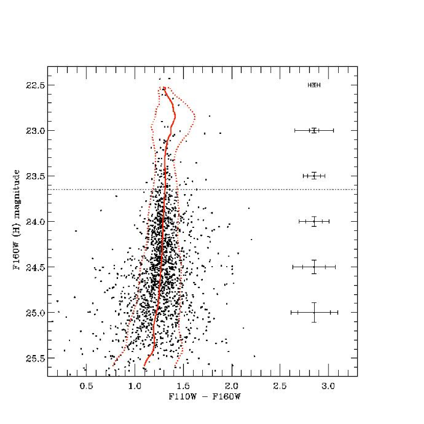
Figure 16: A1: Color magnitude diagram for artificial star images where all stars have $F110W-F160W=1.30$. The recovered RGB is widened by crowding over purely photometric errors, but is still significantly narrower than the observed spread (Figure 8).

The spread in color of the recovered artificial stars is nearly as great as the observed spread, but this results from the combined effects of crowding and the intrinsic color spread of the real stars. To determine the amount of spread in the RGB directly caused by crowding, we created two new artificial images. Beginning with the residual noise images left after PSF subtraction by allstar, we added back artificial stars at the same locations as all the detected stars; for the $F160W$ image, we used the detected magnitudes, effectively reconstructing the original $F160W$ image, but with a little extra Poisson noise which addstar includes. For the $F110W$ image, we added stars at all the locations of the detected stars, but adjusted their magnitudes so that every star had the same color, $F110W-F160W=1.3$, about the mean of the RGB. Running the daophot suite on these images in a manner identical to that used on the real data produces the CMD in Figure A1; this figure should be compared to the real data CMD of Figure 9. The recovered spread of the artificial RGB is greater than the median photometric errors, but is quite a bit less than the observed RGB width of NGC3379.

Figure 17: A2: Histograms comparing the color spread of the monochromatic artificial RGB (with $F110W-F160W=1.30$) to the real stars at four magnitude intervals starting at the RGB tip. The solid line Gaussians are best fits to the plotted histograms; the dashed line Gaussians have the same total area, but the widths of the real star distributions in Figure 9. The intrinsic color spreads are estimated as the quadrature difference of the observed and monochromatic artificial star color spreads.

In Figure A2, we compare the artificial data color spread to the actual observed color spread, using the same magnitude intervals as in Figure 12. The quadrature difference in color spread between the real and artificial images is our estimate of the intrinsic width of the RGB. The intrinsic color spread increases from 0.20 at the RGB tip to 0.30 at the limit of our data; this is consistent with the presence of a very metal poor population entering at fainter magnitudes, as predicted by the isochrones in a composite metallicity population (c.f. Figure 11).

The artificial RGB should have a mean color of exactly 1.3, but the measured color moves 0.06 magnitudes bluer at $F160W=24.65$, where we are 80% complete, and 0.16 magnitudes bluer in the confusion-limited regime. The reddest faint stars go undetected in $F110W$, which causes the shift to bluer colors and accounts for the difference between the mean location of the observed RGB and the Girardi isochrones at faint magnitudes (Figures 10, 11).

Table 4: Artificial Star Photometry Tests

Input			Recovered (Input $F110W-F160W=1.1$)
$F160W_{inp}$	$F110W_{inp}$		%rec	$<color>$	$\sigma_{color}$	$<F160W>$	$\sigma_{F160W}$	$<F110W>$	$\sigma_{F110W}$
22.75	23.85		99.7	1.102	0.061	22.750	0.053	23.848	0.055
23.00	24.10		99.7	1.104	0.077	22.998	0.068	24.096	0.069
23.25	24.35		99.8	1.102	0.091	23.243	0.084	24.340	0.086
23.50	24.60		99.4	1.106	0.115	23.493	0.101	24.589	0.102
23.75	24.85		99.0	1.107	0.143	23.735	0.128	24.836	0.132
24.00	25.10		97.4	1.111	0.172	23.977	0.156	25.073	0.162
24.25	25.35		94.8	1.113	0.217	24.214	0.194	25.310	0.198
24.50	25.60		88.3	1.121	0.248	24.427	0.237	25.519	0.239
24.75	25.85		77.3	1.156	0.280	24.609	0.276	25.709	0.293
25.00	26.10		63.0	1.198	0.323	24.735	0.328	25.861	0.366
25.25	26.35		51.8	1.230	0.326	24.762	0.429	25.921	0.421
25.50	26.60		45.4	1.231	0.321	24.695	0.547	25.895	0.517
25.75	26.85		43.2	1.246	0.312	24.634	0.580	25.837	0.560
Input			Recovered (Input $F110W-F160W=1.5$)
22.75	24.25		99.8	1.496	0.071	22.750	0.053	24.245	0.078
23.00	24.50		99.7	1.496	0.091	22.998	0.068	24.492	0.098
23.25	24.75		99.7	1.490	0.112	23.244	0.084	24.731	0.124
23.50	25.00		99.4	1.488	0.140	23.493	0.101	24.977	0.147
23.75	25.25		98.8	1.486	0.169	23.735	0.128	25.222	0.186
24.00	25.50		97.1	1.476	0.209	23.977	0.157	25.447	0.228
24.25	25.75		94.0	1.465	0.256	24.214	0.194	25.668	0.273
24.50	26.00		87.0	1.437	0.280	24.426	0.237	25.846	0.319
24.75	26.25		75.7	1.424	0.311	24.601	0.280	25.987	0.390
25.00	26.50		61.5	1.393	0.340	24.711	0.347	26.057	0.460
25.25	26.75		51.0	1.364	0.328	24.712	0.468	26.024	0.525
25.50	27.00		45.9	1.322	0.340	24.656	0.564	25.948	0.588
25.75	27.25		42.9	1.292	0.313	24.603	0.574	25.868	0.571

10 Appendix B: NICMOS Color Transformations

To compare NICMOS data with ground-based IR photometry for stars in globular clusters and the Milky Way bulge requires a rather severe transformation because $F110W$ is much wider and extends well to the blue of standard $J$-band filters. A number of transformations have been published, but none were suitable for our purposes, either because they did not reliably extend to cool giants (Origlia & Leitherer 2000; Marleau et al. 2000) or were based on outdated NICMOS photometry zeropoints (Stephens et al. 2000).

To derive an improved transformation, we used the Girardi isochrones themselves, which are available in both ground-based Bessell-Brett (1988) and NICMOS IR colors. In keeping with our finding that the stellar population of NGC3379 is relatively old and metal rich, and to obtain the reddest possible points along a well-developed giant branch, we base the transformation on the 14 Gyr isochrones of various abundances. Comparison of the isochrones in the two photometric systems shows that there is little dependence of the transformation on metallicity or age and also that the transformation relation clearly differs from the linear approximation of Marleau et al. (2000) by up to nearly 0.2 magnitudes for $J-H>0.7$ (Figure B1). To derive our improved transformation, we fit a high order polynomial to the isochrone-isochrone comparison and then extended the transformation linearly using the two reddest NICMOS photometric standards, OPH-S1 and CSKD-12 (Figure B1). Our reliance on a linear extrapolation for colors redder than $F110W-F160W=1.4$ is again probably an oversimplification, but there are no additional data that can be called into play.

Figure 18: B1: Ground-based Bessell-Brett $J-H$ to NICMOS $F110W-F160W$ transformation (heavy solid line) derived from the Girardi isochrones for 14 Gyr and a range of abundances; from [Fe/H]$=-2.27$ to +0.2, there is little metallicity dependence of the photometric transformation. The individual isochrone points are plotted as crosses; there are no points redder than what is shown. The reddest NICMOS photometric standards (filled triangles) are used to extend the transformation linearly. The M9.5V star BRI B0021-02 is labeled; its 2MASS $J$ and $H$ magnitudes transformed to the Bessell-Brett system (filled triangle) are in better agreement with the isochrones than the photometry from the NICMOS STScI website (open triangle). The transformation adopted by Marleau et al. (2000) is shown as the light solid line.

Comparison with the four blue NICMOS standard star calibration data ($J-H<1.$) shows that the isochrone-derived transformation yields a good relation. There has been some uncertainty concerning the correct ground-based $J$-band photometry of the NICMOS standard BRI B0021-02. We have placed it in Figure B1 using the $J-H$ color from the 2MASS data base, transformed to the BB system using equations obtained at the 2MASS website (http://www.ipac.caltech.edu/2mass). The star’s location is consistent with the isochrones. The ground-based photometry listed at the NICMOS STScI website, however, places BRI B0021-02 about 0.15 magnitudes to the blue in the BB system (open triangle in Figure B1). Marleau et al. (2000) use an even bluer color for this star in deriving their linear transformation equation (see their Figure 6 and Appendix), which perhaps led them to adopt a color transformation considerably steeper than ours.

To test our transformation, we compared the IR photometry data of Frogel et al. (1981) for 47 Tuc to the appropriate Girardi isochrones. The Frogel et al. data are on the CIT photometric system, so it is necessary to apply the mild 10% transformation from CIT to the Bessell-Brett system given in Marleau et al. (2000). The left panel of Figure B2 shows the resulting excellent fit of the 47 Tuc IR giant branch by the 14 Gyr, [Fe/H]$=-0.7$ Girardi isochrone, adopting $m-M=13.27$ for 47 Tuc; these numbers are consistent with prevailing views of the stellar population of this cluster (e.g. Hesser et al. 1987). In the right panel, we have transformed the cluster data points to the NICMOS system using our derived transformation (Figure B1) and over-plotted them on the same Girardi isochrone for the NICMOS bandpasses. Using our isochrone-derived transformation, the 47 Tuc data, perhaps not surprisingly, are still well-described by the same age and metallicity isochrone in the NICMOS system. This is not a trivial result, however; we have not applied the transformation to the isochrones, only to the cluster data. The isochrones in the different photometric systems are produced by direct convolution of theoretical spectral energy distributions with filter transmission curves. The transformation we have derived is in this sense a wholly theoretical one, but it works well and is consistent with the four NICMOS standards that overlap the isochrone color range. Other published empirical ground-based–to–NICMOS photometric transformations, however, result in large discrepancies of the 47 Tuc data with the proper isochrone at these red colors. The Marleau et al. transformation, for instance, makes 47 Tuc appear to be solar metallicity (Figure B2), in conflict with all published results for this cluster.

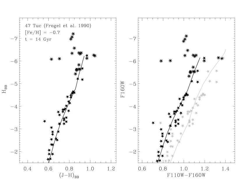
Figure 19: B2: The left panel shows that the Girardi et al. 14 Gyr isochrone for [Fe/H]$=-0.7$ (solid line) is an excellent fit to the infrared data of 47 Tuc from Frogel et al. (1990), after transformation of the data to the Bessell-Brett (1988) system (stars; known variables are circled). In the right panel, the 47 Tuc points have been transformed to the NICMOS system using the transformation derived from the Girardi isochrones; the excellent agreement with the isochrone is preserved. Applying the transformation given by Marleau et al. (2000), however, to transform the data to the NICMOS system results in the RGB of 47 Tuc being too red (grey stars), making 47 Tuc appear to match a 14 Gyr, solar abundance isochrone (grey line; variables omitted for clarity).

References

- (1) Arimoto, N. 1996, in From Stars to Galaxies, ASP Conference Series 98, Leitherer, C., Fritze-von Alvensleben, U., & Huchra, J., eds.
- (2) Bekki, K., Couch, W. J., Drinkwater, M. J., & Gregg, M. D. 2001, ApJL, 557, 39.
- (3) Bertelli, G., Bressan, A., Chiosi, C., Fagotto, F., & Nasi, E. 1994, A&AS, 106, 275
- (4) Blanco, B. M. 1984, AJ, 89, 1836
- (5) Buta, R. J. & McCall, M. L. 2003, AJ, 125, 1150
- (6) Capaccioli, M., Held, E.V., Lorenz, H. & Vietri, M., 1990, AJ, 99, 1813
- (7) Capaccioli, M., Vietri, M., Held, E. V., & Lorenz, H. 1991, ApJ, 371, 535
- (8) Davidge, T. J. 2002, AJ, 124, 2012
- (9) Davies, R. L., Burstein, D., Dressler, A., Faber, S. M., Lynden-Bell, D., Terlevich, R. J. and Wegner, G. 1987, ApJS, 64, 581
- (10) Davies, R. L., Sadler, E. M., & Peletier, R. F. 1993, MNRAS, 262, 650
- (11) de Vaucouleurs, G. & Capaccioli, M. 1979, ApJS, 40 699
- (12) Elston, R. & Silva, D. 1992, AJ, 104, 1360
- (13) Faber, S. M., 1973, ApJ, 179, 423
- (14) Faber, S. M. et al. 1997, AJ, 114, 1771
- (15) Freedman, W. L. 1989, AJ 98, 1285
- (16) Freedman, W. L. 1992, AJ 104, 1349
- (17) Freedman, W. L. et al. 2001, ApJ 553, 47
- (18) Frogel, J. A., Persson, S. E., & Cohen, J.G. 1981 ApJ, 246, 842
- (19) Frogel, J. A., Persson, S. E., & Cohen, J.G. 1983 ApJS, 53, 749
- (20) Frogel, J. A. 1983 ApJ, 272, 167
- (21) Frogel, J. A., Terndrup, D. M., Blanco, V. M., & Whitford, A.E. 1990, ApJ, 353, 494
- (22) Frogel, J. A. & Whitford, A. 1987 ApJ, 320, 199
- (23) Fruchter, A. S. & Hook, R. N. 2002, PASP, 114, 144
- (24) Gibson, B. K. et al. 2000, ApJ, 529, 723
- (25) Girardi, L., Bertelli, G., Bressan, A., Chiosi, C., Groenewegen, M. A. T., Marigo, P., Salasnich, B., & Weiss, A. 2002, A&A, 391, 195
- (26) Graham, J. A. et al. 1997, ApJ, 477, 535
- (27) Gregg, M. D. 1992, ApJ, 384, 43
- (28) Gregg, M. D. 1995, ApJ, 443, 527
- (29) Gregg, M. D. 1997, New Astronomy, 1, 363
- (30) Grillmair, C. et al. 1996, AJ, 112, 1975
- (31) Guarnieri, M. D., Renzini, A., & Ortolani, S. 1997, ApJL, 477, 21
- (32) Harris, G. L. H., Harris, W. E., & Poole, G. B. 1999, AJ, 117, 855
- (33) Hesser, J. E., Harris, W. E., Vandenberg, D. A., Allwright, J. W. B., Shott, P., & Stetson, P. B. 1987 PASP, 99, 739
- (34) Hjorth, J. & Tanvir, N. R. 1997, ApJ, 482, 68
- (35) Hughes, S. M. G., Wood, P. R. 1990, AJ, 99, 784
- (36) Krist, J. 1993, in ASP Conf. Ser. 52: Astronomical Data Analysis Software and Systems II, ed. R. J. Hanisch, R. J. V. Brissendon, & J. Barnes, (San Francisco: ASP), 536
- (37) Liu, M. C., Charlot, S. & Graham, J. R. 2000, ApJ, 543, 644
- (38) Leitherer, C., et al. 1996, in ASP Conf. Ser. 98: From Stars to Galaxies, ed. Leitherer, C., Fritze-von Alvensleben, U., & Huchra, J., (San Francisco: ASP)
- (39) Luppino, G. A. & Tonry, J. L. 1993, ApJ, 410, 81
- (40) Maihara, T., et al. 2001, PASJ, 53, 25
- (41) Maeder, A., Meynet, G. 1989, A&A, 210, 155
- (42) Méndez, R. A.; Minniti, D. 2000, ApJ, 529, 911
- (43) Minniti, D., Olszewski, E.W., Liebert, J. W., White, S. D. M., Hill, J. M., & Irwin, M. 1995, M.N.R.A.S, 277, 1293.
- (44) Nieto, J.-L. & Prugniel, P. 1987, A&A, 186, 30
- (45) Pastoriza, M. G., Winge, C., Ferrari, F., Macchetto, F. D., & Caon, N. 2000, ApJ, 529, 866
- (46) Peletier, R. F. et al. 1999, MNRAS, 310, 863
- (47) Rejkuba, M., Minniti, D., Silva, D. R., & Bedding, T. R. 2001, A&A, 379, 781
- (48) Rejkuba, M., Minniti, D., Courbin, F., & Silva, D. R. 2002, ApJ, 564, 688
- (49) Rejkuba, M., Minniti, D., & Silva, D. R. 2003, A&A, in press (astro-ph/0305432)
- (50) Renzini, A. 1998, AJ, 115, 2459
- (51) Rich, R. M. 1988, AJ, 95, 828
- (52) Rose, J. A. 1985, AJ, 90, 1927
- (53) Sadler, E. M., Rich, R. M., Terndrup, D. M. 1996, AJ, 112, 171
- (54) Sadler, E. M. & Gerhard, O. E. 1985, MNRAS, 214, 177
- (55) Sakai, S., Madore, B. F., Freedman, W. L., Lauer, T. R., Ajhar, E. A., & Baum, W. A. 1997, ApJ, 478, 49
- (56) Schlegel, D. J., Finkbeiner, D. P., & Davis, M. 1998, ApJ, 500, 525
- (57) Schneider, S. E. 1989, ApJ, 343, 94
- (58) Soria, R., et al. 1996, ApJ 465, 79
- (59) Schweizer, F. & Seitzer P. 1992, AJ, 104, 1039
- (60) Statler, T. S. 1994, AJ, 108, 111
- (61) Statler, T. S. 2001, AJ, 121 244
- (62) Statler, T. S. & Smecker-Hane, T. 1999, ApJ, 117, 839
- (63) Tanvir, N. R., Ferguson, H. C., Shanks, T., 1999, MNRAS, 310, 175
- (64) Terlevich, A. I. & Forbes, D. A. 2002, MNRAS, 330, 547
- (65) Thompson, R. I., Rieke, M., Schneider, G., Hines, D. C. & Corbin, M. R. 1998, ApJL, 492, L95
- (66) Tiede, G. P., Frogel, J. A., & Terndrup, D. M. 1995, AJ, 110, 2788
- (67) Tonry, J. L., Ajhar, E. A., & Luppino, G. A. 1990, AJ, 100, 1416
- (68) Van den Bergh, S. 1989, PASP, 101, 1072
- (69) Williams, R. E., et al. 1996, AJ, 112, 1335
- (70) Worthey, G. & Ottaviani, D. L. 1997, ApJS, 111, 377