Modelling galactic spectra: I - A dynamical model for NGC 3258

Abstract

In this paper we present a method to analyse absorption line spectra of a galaxy designed to determine the stellar dynamics and the stellar populations by a direct fit to the spectra. This paper is the first one to report on the application of the method to data. The modelling results in the knowledge of distribution functions that are sums of basis functions. The practical implementation of the method is discussed and a new type of basis functions is introduced.

With this method, a dynamical model for NGC 3258 is constructed. This galaxy can be successfully modelled with a potential containing 30% dark matter within $1r_{e}$ with a mass of $1.6\times 10^{11}M_{\odot}$. The total mass within $2r_{e}$ is estimated as $5\times 10^{11}M_{\odot}$, containing 63% dark matter. The model is isotropic in the centre, is radially anisotropic between 0.2 and 2 kpc ($0.88r_{e}$) and becomes tangentially anisotropic further on. The photometry reveals the presence of a dust disk near the centre.

1 Introduction

It is well known that in galaxies stellar populations and stellar dynamics cannot be studied completely independently; the determination of the line profiles and kinematic parameters depends on assumptions about the dominant stellar population, while the determination of the chemical properties depends on the absorption strenght of the spectral lines.

In general, stellar kinematics are retrieved by comparing the observed spectra with the convolution of a stellar template spectrum with a model line-of-sight velocity profile, see De Bruyne et al., (2003) for a discussion of some standard techniques. The stellar template belongs to the same spectral class as the dominant stellar population in the galaxy, or can be a mix of different stellar type spectra. Often, a best matching stellar mix is determined for the spectrum at the centre, and this mix is then used throughout the whole galaxy. In some cases, the stellar mix is allowed to vary with radius, (e.g. Carter et al., (1999)). However, the only criterion used for obtaining a proper mix is a good fit, without any physical considerations. Therefore, it is acknowledged that this procedure does generally not yield a reliable population synthesis.

The kinematics obtained from a parametrization of the line-of-sight velocity distributions can be used as input for a dynamical model. Within this multistep scheme of dynamical modelling, it is acknowledged that dynamical evidence for dark matter in elliptical galaxies requires the use of more information contained in the line-of-sight velocity distribution (hereafter LOSVD) than simply the mean velocity and velocity dispersion. The reason for this is the existence of a so called mass-anisotropy degeneracy. In a dynamical model it is possible to mimic the influence of a dark matter halo by tangential anisotropy. Therefore, also the anisotropy information in LOSVDs should be used. However, there is no uniformity in the parametrization of these LOSVDs and different algorithms may well have different biases (Joseph et al., 2001). Moreover, it is not always straightforward to include these parameters in a fit, since not all of them are linearly dependent on the distribution function (hereafter DF) (Gerhard et al. (1998), De Bruyne et al., (2001)). Another option is to use the complete LOSVD as dynamical input. This omits the need to approximate the LOSVD with a number of parameters, but in combination with the Schwarzschild orbit superposition method, this requires a careful smoothing both of the LOSVD and the dynamical model (Gebhardt et al., 2000). But there is still another way of dealing with the kinematic information of a galaxy, through direct modelling of the observed spectra.

In this paper we adopt a method to analyse spectra from elliptical galaxies that explores the dynamics of the galaxy and simultaneously offers a way to study the stellar populations in that galaxy. The method originates from the field of dynamical modelling and is outlined by De Rijcke & Dejonghe (1998), hereafter DD98. The main idea is that the different stellar populations that contribute to the integrated galaxy spectrum do not necessarily share the same kinematic characteristics. Hence, in terms of dynamical modelling, they should be associated with different distribution functions. A simultaneous determination of the best stellar mix and the best distribution functions associated with them de facto amounts to a dynamical model and a stellar population synthesis.

This paper is the first to present the application of the modelling method to data. The aim is to determine the gravitational potential of NGC 3258, by modelling the galaxy spectra using different stellar templates. The modelling strategy is outlined and commented, and a new family of dynamical components is presented.

This is the first paper in a series of two, where a deeper interplay between dynamics and population synthesis is explored. In this first paper, the attention will be focused on the dynamical modelling aspect, while the second paper will go deeper into the stellar population analysis.

In the next section, the observations and data reduction steps are presented. The modelling strategy is outlined in section 3. Section 4 presents the dynamical components that were used. In section 5 the results of the modelling are presented. Section 6 contains a discussion of the results and the conclusions can be found in section 7.

2 Observations and data reduction

The E1 galaxy NGC 3258 is one of the brightest members of the Antlia Group. In its neighborhood, NGC 3257 can be found at 4.5 arcmin (about $21r_{e}$) and NGC 3260 is at 2.6 arcmin (about $12r_{e}$). We measured a systematic velocity of 2709 km/s, this puts NGC 3258 at a distance of 36.12 Mpc (taking $H_{0}=75\rm{km/s/Mpc}$). This means that a linear size of 1 kpc at the distance of NGC 3258 translates into an angular size of $5.7^{\prime\prime}$.

NGC 3258 was observed with the ESO-NTT telescope in the nights of 27-28/2/2000. Spectra of the major axis covering the Ca II triplet around 8600 Å were taken. During the observations in 2000, also imaging of NGC 3258 in the R band was performed. The detector used for this observation run was a Tektronix CCD with $2048\times 2047$ pixels, 24$\mu m\times$24$\mu m$ in size and with a pixel scale of $0.27^{\prime\prime}$/pix. Another observation run, in 1999, was used to obtain images in the B band.

2.1 Photometry

R band observations (in total 600 sec integration time) of NGC 3258 were obtained at the ESO-NTT using the red arm of EMMI during the spectroscopic run in februari 2000. An additional B band image (600 sec integration time in total) was obtained in february 1999 in the same configuration. The detector used for the B band images was a Tektronix CCD with 1024$\times$1024 pixels, 24$\mu m\times$24$\mu m$ in size and with a pixel scale of $0.37^{\prime\prime}$/pix.

The seeing (judged from a number of stars in the images) was $1.1^{\prime\prime}$ for the R band images and $1.7^{\prime\prime}$ for the B band images. The photometric zero point was established by comparison with published photometric data available on NED. Figure 1 shows an image of NGC 3258, isophotes are plotted in figure 2. In this figure, the central isophote seems to be a little displaced compared to the other isophotes. Both B and R images show a slightly off-centre nucleus, with a shift of about $0.45^{\prime\prime}$ (or 0.07 kpc) in the horizontal direction and a shift of about $0.1^{\prime\prime}$ (or 0.01 kpc) in the vertical direction. This is illustrated in the upper panel figure 5, where the shift of the centres of the isophotes is shown.

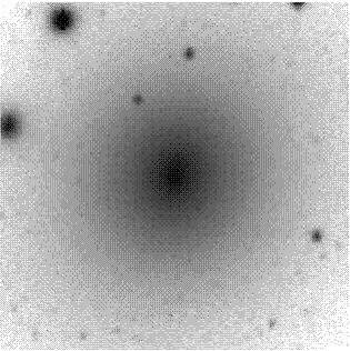
Figure 1: B band image of NGC 3258, the size of the region is $110^{\prime\prime}\times 110^{\prime\prime}$. North is up and east is to the left.

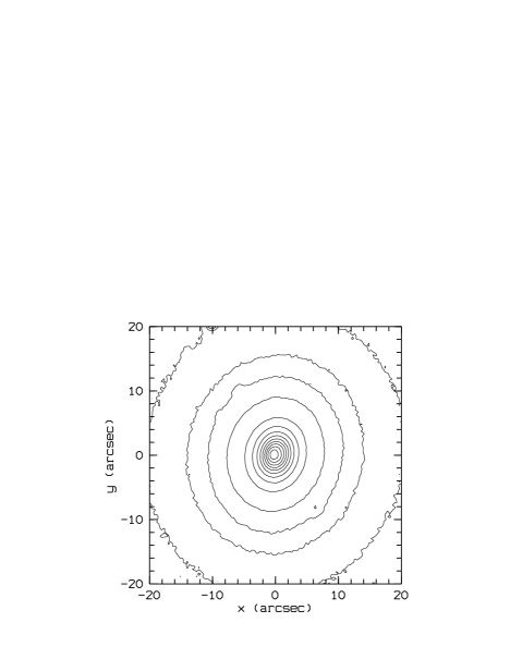
Figure 2: Isophotes of NGC 3258.

The photometric parameters were derived by fitting elliptic isophotes to the image. The intensity along the isophotes was expanded in a fourth order Fourier series, in order to reveal deviations from pure elliptic isophotes, like in e.g. De Rijcke et al. (2003). In figure 3, the main photometric parameters are shown: surface brightness, position angle, ellipticity and B-R profile as derived from the B and R surface brightness profiles in the left column. The coefficients indicating deviations from pure elliptic isophotes are shown in the right column. The values for these coefficients indicate that NGC 3258 is an almost perfect elliptical galaxy, with an ellipticity between 0.1 and 0.2.

A Sérsic profile ($I(r)=I_{0}\exp[-(r/r_{0})^{1/n}]$, with $I(r)$ the surface brightness profile, $I_{0}$ the central surface brightness, $r_{0}$ the scale length, an $n$ the Sérsic parameter (Ciotti et al.,, 1995) was fitted to the surface brightness, the result of the fit is overplotted (in solid line) in the upper left panel of figure 3. The observed surface brightness profile can be well matched with a Sérsic profile with Sérsic parameter $n=5.47\pm 0.07$. The effective radius is $12.95^{\prime\prime}$ or 2.26 kpc.

Values for B-R (derived from the photometric profiles) are shown in the lower left panel of figure 3. Within the central $5^{\prime\prime}$, there seems to be a slight reddening of the nucleus. B-R changes from about 1 in the most central measurement to about 0.85 at $5^{\prime\prime}$.

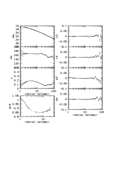
Figure 3: Photometric parameters for NGC 3258. Left column, from top to bottom: surface brightness, position angle, ellipticity and B-R. Right column, the coefficients indicating deviations from pure elliptic isophotes.

2.2 Central dust component

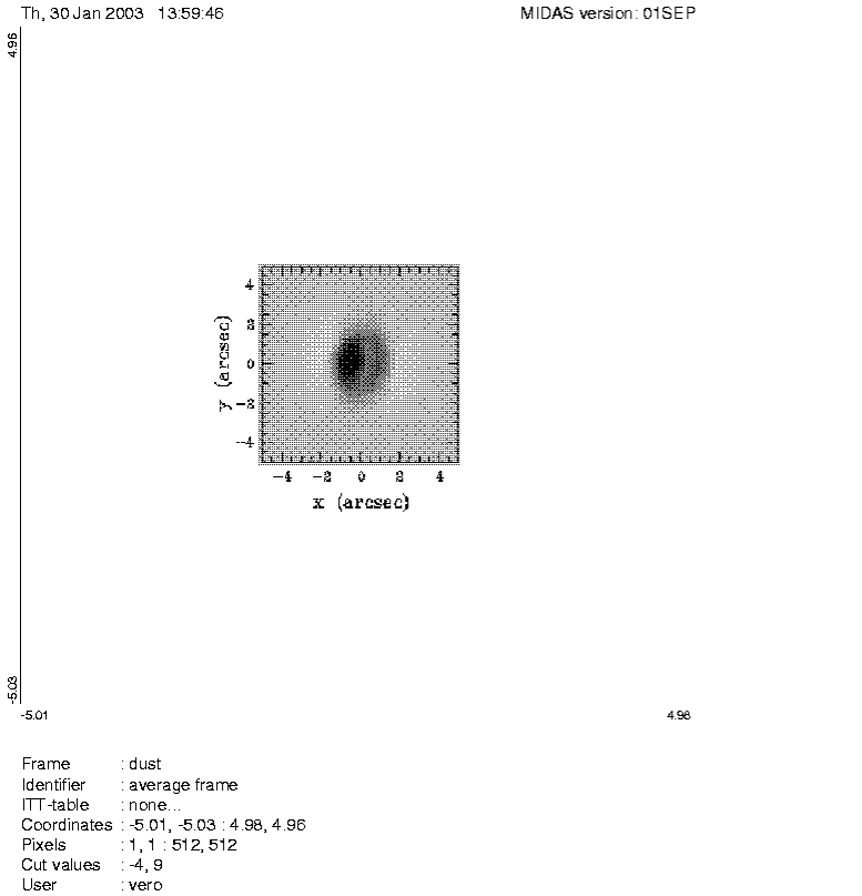
Figure 4: Inverted image of the central part of the unsharp masked R image. The light grey band in the centre is a central dust disk.

Figure 4 shows the central part of the unsharp masked R image with a clearly visible dust feature. The estimated radius of the major axis of the disklike feature is about $1^{\prime\prime}$ - $1.5^{\prime\prime}$ (0.17 kpc - 0.26 kpc). Figure 5 shows a contour map of this region (lower panel) and a cut along a horizontal line through the centre (upper panel). This line does not coincide with any of the photometric axes. The effect of the dust lane on the apparent brightness is clearly visible in the upper panel of that figure. The brightest central point does not coincide with the centre of the isophotes for the main body of the galaxy. The same behaviour is seen in the B band images. The off-centre nucleus appearing in the B and R images is probably due to the obscuring effect of the dust lane.

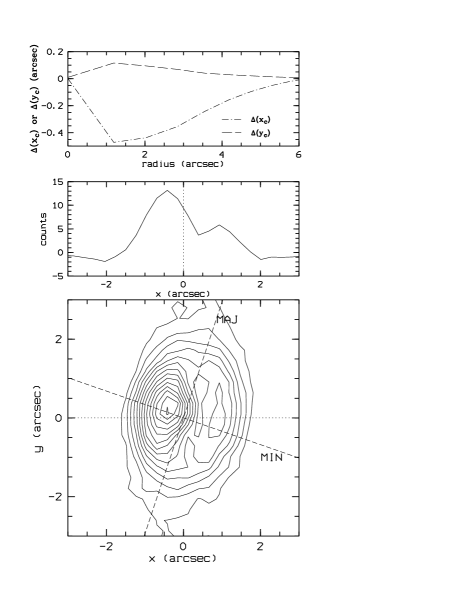
Figure 5: Upper panel: displacement in x ($\Delta(x_{c})$) and y ($\Delta(y_{c})$) direction of the centre of the isophotes as function of the major axis of the isophotes. Middle panel: The intensity profile along the cut with a horizontal axis through the galaxy centre (dotted line in lower panel). Lower panel: contours of the central part of the unsharp masked R image. The photometric major and minor axis are plotted in dashed line.

2.3 Spectroscopy

For the spectra, grating #7 was used, having a dispersion of 0.66 Å/pix. A slit width of $1.5^{\prime\prime}$ yielded a spectral resolution of 3.67 Å FWHM, resulting in an instrumental dispersion of about 54 km/s in the region of the Ca II triplet. For NGC 3258, several exposures of 3600 sec were taken (in total 11 hours).

A number of standard stars (G dwarfs and K and M giants) were also observed, they are listed in table 1.

Standard reduction steps were applied to these spectra with ESO-MIDAS . Dedicated exposures, taken during both runs, were used for bias correction, dark correction and flatfielding. Cosmic ray hits were removed using a top hat filter. After this correction, remaining cosmics were also removed by hand.

For the wavelength calibration, lamp spectra were taken just before or after each of the spectroscopic observations of the galaxy or the stellar template stars. For each row in the spectra a polynomial was constructed to transform the pixel scale into wavelength scale. The calibrated images with the Ca II triplet have a step of $0.3$Å.

Airmass correction is applied, using the mean value of the airmass at the beginning and end of the exposure. The contribution of the sky to the spectra was estimated from an upper and lower region of the image, where there was no contribution of the light of the galaxy or template star. Several galaxy spectra were reduced separately, aligned and combined into one galaxy spectral image.

2.4 Kinematic parameters

In figure 6 kinematic parameters are presented. These parameters are derived from the spectra, using a $\chi^{2}$ minimization technique in order to find the parameters of a truncated Gauss-Hermite series that gives the best approximation to the LOSVD. The spectra were spatially rebinned to satisfy a minimum S/N. Only data points from the side of the galaxy with mean streaming away from the observer are shown. A best fitting template mix (i.e. the one that gives the smallest $\chi^{2}$ in the fitting) was determined for the central data point and this mix was then used throughout the whole galaxy. The spectra are analysed with a mix of a G5V dwarf and a K4III giant.

The kinematic parameters are determined following the method of van der Marel & Franx (1993) and implemented as in De Rijcke et al. (2003), first fitting a Gaussian LOSVD to determine $\langle v\rangle$ and $\sigma$, and then keeping these lowest order parameters fixed to fit the other coefficients.

If $\langle v\rangle$, $\sigma$, $h_{3}$ and $h_{4}$ are the lowest order parameters for the LOSVD, the true moments are approximated more accurately by

$$\langle v_{p}\rangle=\langle v\rangle+\sqrt{3}\sigma h_{3}$$ (1)

for the first order moment and

$$\sigma_{p}=\sigma(1+\sqrt{6}h_{4})$$ (2)

for the second order moment, $\langle v_{p}\rangle$ and $\sigma_{p}$ are also called the ’corrected’ values.

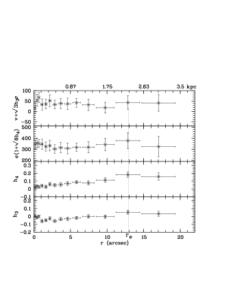
Figure 6: Kinematics obtained from the spectral feature around 8600 Å.

These data are consistent with the kinematic parameters presented by Pellegrini et al. (1997) and Koprolin & Zeilinger (2000).

HD 21019	G2V
HD 115617	G5V
HD 102070	G8III
HD 117818	K0III
HD 114038	K1III
HD 44951	K3III
HD 29065	K4III
HD 99167	K5III
HD 129902	M1III
HD 93655	M2III

Table 1: Observed stellar templates.

2.5 Other observations

NGC 3258 is a weak but extended radio source with a total flux of 18.3 mJy (VLA observations at 4.9 GHZ (6 cm) within $45^{\prime\prime}$) (Sadler et al., 1989), where the core ($<5^{\prime\prime}$) flux is only $7\%$ of the total flux. A hot gaseous corona around NGC 3258 emits about $3\times 10^{41}\rm{ergs}s^{-1}$ (Fabiano et al., 1992). There are no total mass estimates based on X-ray observations available.

Bregman et al. (1998) studied this galaxy in the far-infrared, and derived a dust temperature of 24.5 K and a dust mass of $6\times 10^{6}M_{\odot}$ from IRAS observations at 60 and $100\mu\rm{m}$. This is not unlike what is found in spiral galaxies. The mid-infrared properties of NGC 3258, based upon ISOCAM observations at 6.75, 9.63 and $15\mu\rm{m}$, indicate the presence of a hot $T\simeq 260$K) dust component (Ferrari et al., 2002). A mass of $48M_{\odot}$ of hot dust within a radius of 5.5 kpc was derived. This is at the lower end of the typical range of 10-400 $M_{\odot}$ reported for early-type galaxies.

Furthermore, the galaxy shows [OII] emission (Bettoni & Buson,, 1987) and weak HI emission (Jenkins, 1983).

3 Dynamical modelling strategy

There is a large variety of ways to make a dynamical model and there also different strategies to use these models. For a recent review, see Dejonghe & De Bruyne, (2003).

The data used for the modelling are the projected surface brightness and a set of spectra of the galaxy, taken at several positions along the major axis. The projected surface brightnes is used to obtain a graviational potential, this is described in more detail in 5.1.

An important issue for the modelling strategy applied in this paper, is the form of the data that are used to determine the DF. In this case, the fit is done directly to the spectra (after necessary data reduction steps). This means that the observed quantities that have to be reproduced by the model are pairs (wavelength, flux). The use of spectra as input for dynamical information is in contrast with more frequently used modelling techniques where a number of kinematic parameters are first derived from the spectra. The models are then fitted to these parameters that are moments of the distribution function. The modelling procedure used in this paper is described in detail in DD98. The input spectra are reproduced by a dynamical model that uses spectra of different template stars. An important characteristic of these models is that they provide a DF for each population that is used in the model.

This is a function which gives the probability to find a star on an orbit characterized by the integrals of motion $E$ (the energy), $L$ (the total angular momentum) and $L_{z}$ (the component of the angular momentum along the rotation axis of the system). This function holds all information on the dynamical state of the galaxy.

The resulting DF for each type of star is a sum of basic components and is constructed with a quadratic programming algorithm (Dejonghe,, 1989). There are two main requirements for the DF: (1) the difference between the observed quantities and the quantities calculated from the DF should be minimized (least squares minimization) and (2) the DF should be a positive function.

Modelling the spectra instead of kinematic parameters causes a considerable increase in the number of data points and hence an increase of the required computing time, but there are a number of advantages over using kinematic parameters.

• More traditional modelling involves a two step process (e.g. De Bruyne et al., (2001)): first determining kinematic parameters out of observed spectra and then calculating a model. Here this is turned into a one step process. Omitting the step of determining kinematic parameters and using the galactic spectra as input has the consequence that the kinematic information used as input for the modelling is independent of any parameterization. Also in the more traditional two step modelling process, there are some non-parametric methods to derive kinemtical profiles, see De Bruyne et al., (2003).

  Of course, the dynamical profiles that are a result from the modelling depend on the assumptions concerning the gravitational potential and the dark matter halo, but this is the case for every dynamical modelling technique. In this paper, the gravitational potential is assumed to be spherical. This assumption is not a conceptual issue but is justified by the shape of the NGC 3258.

• Furthermore, since the basis distribution functions that are used in the fit are chosen freely by the algorithm from a large library, also the modelling procedure itself is non-parametric. The smoothness of the model is guaranteed by the use of smooth basis functions. Hence, considering also the previous remark, this method can be regarded as a non-parametric modelling method. Moreover, the model has considerably more freedom in determining LOSVDs than can be achieved with a limited number of parameters as is the case when kinematic parameters are determined in a separate process.

• The modelling process based on quadratic programming, uses a $\chi^{2}$ (see equation (10) in DD98) that has the statistical meaning of a goodness of fit indicator if the noise on the spectra is Poisson noise and the data points are weighted accordingly.

• The Hessian matrix (see equation (13) in DD98) involved in the quadratic programming can be used to calculate error bars on the distribution functions that have a statistical meaning and give an idea of the uncertainty on the model and on its moments. Tests with synthetic spectra (DD98) show that the error bars are a reliable measure for the spread between input model and fit, as caused by the adopted Poisson noise. Moreover, if the component library is sufficiently complete the systematic errors are negligible compared to the random errors.

• If the dynamical modelling uses different template stars, it can result in a population synthesis.

• The composition of the stellar mix is allowed to vary smoothly as a function of radius and is therefore directly connected to the internal dynamics. This minimizes stellar template mismatch, and allows in meantime to obtain a physical stellar population decomposition.

• Information at different wavelengths can be combined in an elegant way. This is an advantage of using kinematic information on the level of spectra. It is not clear how to interpret profiles of the same kinematic parameters taken from different parts of the spectrum that give different results (van der Marel, 1994).

3.1 Templates

Five template stars that have discernible spectral properties were used: a G2V dwarf, a G5V dwarf, a K1III giant, a K4III giant and a M1III giant (see table 1 for their identification).

The dynamical models were created in an iterative process. First, models were calculated with a single template star, using a library of about 100 dynamical components. Afterward, the components that are selected for the single template models are combined into component libraries that contain a sample of dynamical components for different stellar templates. With these mixed libraries, new models were calculated.

4 Dynamical components

Using a spherical potential in combination with rotating components for the DF, it is possible to obtain a flattened luminous density distribution, as is required to be able to fit the two dimensional surface brightness of this E1 galaxy well. We consider three integral models: $F(E,L,L_{z})$ for which $\sigma_{r}$, $\sigma_{\phi}$ and $\sigma_{\theta}$ are different. These models are linear combinations of three types of components.

4.1 Continuum terms

The continuum of the weighted sum of template spectra does not necessarily fit the continuum of the galaxy spectra. Therefore, low order polynomials are included in the component library to compensate for the small differences between both continua. Such a continuum component has the form

$$g(\ln\lambda,r_{p})=\left({\ln\lambda-\ln\lambda_{1}}\over{\ln\lambda_{2}-\ln\lambda_{1}}\right)^{\alpha}\left({j_{R}(r_{p})-j_{R}(r_{c})}\over{j_{R}(0)}\right)^{\beta},$$ (3)

with $\alpha$ and $\beta$ real numbers, $r_{c}$ the cutoff radius (the component is set to zero for larger radii), $j_{R}(0)$ the central value of the surface brightness, $j_{R}(r_{c})$ the surface brightness at the cutoff radius, $j_{R}(r_{p})$ the surface brightness at the position of the line of sight, $\lambda$ the wavelength at which the spectrum is evaluated, $\lambda_{1}$ and $\lambda_{2}$ bound the spectral region that is used in the fit. The value of $\alpha$ should be small so that these components only fit the continuum and not the absorption lines.

4.2 Fricke components

These components have the following augmented density

$$\tilde{\rho}(\psi,r)=(\psi-E_{0})^{\alpha}\left(r\over r_{c}\right)^{2\beta},\quad\psi\geq E_{0},\;0\;{\rm elsewhere}$$ (4)

with $\alpha$ and $\beta$ positive integers, $r_{c}$ a scale length and $E_{0}$ the energy level at which the component is truncated. All of these components are either isotropic ($\beta=0$) or tangentially anisotropic (component parameter $\beta>0$). However, the coefficients for these components can be negative, hence also radial anisotropic models can be constructed. These are spherical two integral $(E,L)$ components. They have equal velocity dispersions in the tangential directions, $\sigma_{\phi}=\sigma_{\theta}$, but a different radial dispersion in the case of non-isotropic components. A more detailed discussion of this family of components can be found in DD98.

4.3 Rotating components

These components add rotation to the model. Due to the ordered motion of the stars around the component’s symmetry-axis, the tangential dispersion is usually lower than the radial dispersion. These rotating components are axisymmetric two integral $(E,L_{z^{\prime}})$ components (with $z^{\prime}$ the symmetry axis of the component), for which $\sigma_{R}=\sigma_{z^{\prime}}$ and the dispersion in the rotation direction $\sigma_{\phi}$ is different.

In this section, a family of components is introduced that should enable one to reproduce both the rotation of the bulk of the galaxy and the kinematics of a small subsystem, rotating around an axis other than the main galaxy’s rotation axis. The distribution function of the components of this family is given by

$$F(E,L_{z^{\prime}}) = \frac{1}{2^{\beta/2}}(E-E_{0})^{\alpha}\left(i_{\rm rot}L_{z^{\prime}}-L_{0}\right)^{\beta}$$ (5)

$$\hskip 5.0pt\mbox{for }E>E_{0}$$

$$\hskip 5.0pt\mbox{and }i_{\rm rot}=1,\,L_{z^{\prime}}>0\mbox{ and }L_{z^{\prime}}>L_{0}$$

$$\hskip 5.0pt\mbox{or }i_{\rm rot}=-1,\,L_{z^{\prime}}<0\mbox{ and }|L_{z^{\prime}}|>L_{0},$$

with the energy per unit mass $E=\psi(r)-v_{M}^{2}/2-L_{z^{\prime}}^{2}/(2\varpi^{2})$ and the $z^{\prime}$-component of the angular momentum $L_{z^{\prime}}=\varpi v_{\phi}$. The radial distance to the centre is measured by $r$, the distance to the centre measured in the equatorial plane is denoted by $\varpi$. The velocity component in the meridional plane is $v_{M}=\sqrt{v_{\varpi}^{2}+v_{z^{\prime}}^{2}}$, the velocity component perpendicular to the meridional plane is given by $v_{\phi}$. Here, $(x^{\prime},y^{\prime},z^{\prime})$ is a Cartesian reference frame, attached to the component, with the $z^{\prime}$-axis the rotation axis of the component. The overall gravitational potential $\psi(r)$ is taken to be spherical symmetric although the components themselves have an axisymmetric mass distribution. This is acceptable since a small kinematically distinct core probably does not significantly influence the global potential. Also, a slowly rotating elliptical galaxy can still be approximately round, justifying the use of a spherical potential. An axisymmetric potential generally allows $E$ and $L_{z}$ as integrals of motion, with $L_{z}$ the component of the angular momentum parallel to the potentials symmetry axis. Therefore, these components can also be used in an axisymmetric potential if their rotation axis $z^{\prime}$ coincides with the symmetry axis $z$ of the potential.

All the stars have the same sense of rotation, i.e. if $i_{\rm rot}=1$ the stars rotate counter-clockwise, if $i_{\rm rot}=-1$ they rotate clockwise. The parameter $\alpha$ determines the distribution of the stars over orbits with different energies whereas $\beta$ influences the way orbits with different angular momenta are populated. The energy cutoff $E>E_{0}$ will prevent stars from reaching beyond a certain maximum radius. The angular momentum cutoff $|L_{z^{\prime}}|>L_{0}$ on the other hand will impose a minimum radius that stars can reach.

4.3.1 The component’s frame of reference

These components are to be employed in the modelling of slowly rotating, approximately spherical galaxies using a severally symmetric potential. Throughout this work, all dynamical quantities are expressed in spherical coordinates. These particular components however are axisymmetric and their characteristics will be most readily calculated in cylindrical coordinates. Therefore, we seek a transformation linking the spherical coordinates in which the properties of the galaxy as a whole are expressed to a cylindrical coordinate system, attached to each individual component of this family.

First, we introduce a cartesian reference frame ($x,y,z$) with its origin at the galaxy’s centre. The components of a vector $\vec{a}$ in spherical coordinates $(r,\theta,\varphi)$ can be linked to its components in cartesian coordinates via the transformation

$$\left(\begin{array}[]{c}a_{r}\\ a_{\theta}\\ a_{\varphi}\end{array}\right)={\bf A}\left(\begin{array}[]{c}a_{x}\\ a_{y}\\ a_{z}\end{array}\right),$$ (6)

with

$${\bf A}=\left(\begin{array}[]{ccc}\sin\theta\cos\varphi&\sin\theta\sin\varphi&\cos\theta\\ \cos\theta\cos\varphi&\cos\theta\sin\varphi&-\sin\theta\\ -\sin\varphi&\cos\varphi&0\end{array}\right)$$ (7)

Suppose the direction of the rotation axis of the system we are describing, whether it be a small subsystem or the galaxy’s main body, is given by the angles $(\theta_{0},\varphi_{0})$ with respect to the cartesian reference frame. The cartesian coordinate system $(x^{\prime},y^{\prime},z^{\prime})$, fixed to the component, can be obtained by first rotating the $(x,y,z)$-frame over an angle $\varphi_{0}$ around the $z$-axis, yielding the auxiliary $(x^{\prime\prime},y^{\prime\prime},z^{\prime\prime})$-frame, followed by a rotation of the $(x^{\prime\prime},y^{\prime\prime},z^{\prime\prime})$-frame over an angle $\theta_{0}$ around the $y^{\prime\prime}$-axis :

$$\left(\begin{array}[]{c}a_{x}\\ a_{y}\\ a_{z}\end{array}\right)={\bf B}\left(\begin{array}[]{c}a_{x^{\prime}}\\ a_{y^{\prime}}\\ a_{z^{\prime}}\end{array}\right),$$ (14)

with

$${\bf B}=\left(\begin{array}[]{ccc}\cos\theta_{0}\cos\varphi_{0}&-\sin\varphi_{0}&\sin\theta_{0}\cos\varphi_{0}\\ \cos\theta_{0}\sin\varphi_{0}&\cos\varphi_{0}&\sin\theta_{0}\sin\varphi_{0}\\ -\sin\theta_{0}&0&\cos\theta_{0}\end{array}\right).$$ (18)

To facilitate the calculations as much as possible, we will henceforth use cylindrical coordinates $(\varpi,\phi,z^{\prime})$. These are connected to the $(x^{\prime},y^{\prime},z^{\prime})$-frame by the transformation

$$\left(\begin{array}[]{c}a_{x^{\prime}}\\ a_{y^{\prime}}\\ a_{z^{\prime}}\end{array}\right) = \left(\begin{array}[]{ccc}\cos\phi&-\sin\phi&0\\ \sin\phi&\cos\phi&0\\ 0&0&1\end{array}\right)\left(\begin{array}[]{c}a_{\varpi}\\ a_{\phi}\\ a_{z^{\prime}}\end{array}\right)$$ (28)

$$= {\bf C}\left(\begin{array}[]{c}a_{\varpi}\\ a_{\phi}\\ a_{z^{\prime}}\end{array}\right).$$ (32)

One can now immediately make the connection between the spherical coordinates $(r,\theta,\varphi)$ in the galaxy’s reference frame and the cylindrical coordinates $(\varpi,\phi,z^{\prime})$ in the component’s frame of reference using the matrix ${\bf D}={\bf ABC}$ :

$$\left(\begin{array}[]{c}a_{r}\\ a_{\theta}\\ a_{\varphi}\end{array}\right)={\bf D}\left(\begin{array}[]{c}a_{\varpi}\\ a_{\phi}\\ a_{z^{\prime}}\end{array}\right).$$ (33)

4.3.2 The velocity moments

The axisymmetric velocity moments for a counter-clockwise rotating model ($L_{z^{\prime}}\geq 0$, $i_{\rm rot}=1$) are defined as

$$\tilde{\mu}^{+}_{l,m,n}(\psi,\varpi)=$$

$$\int_{-\infty}^{\infty}\int_{-\infty}^{\infty}\int_{-\infty}^{\infty}F(E,L_{z^{\prime}})\,v^{l}_{\varpi}v^{m}_{\phi}v^{n}_{z^{\prime}}\,dv_{\varpi}\,dv_{\phi}\,d_{z^{\prime}}$$ (34)

with $E=\psi(\sqrt{\varpi^{2}+z^{\prime 2}})-\frac{v^{2}}{2}$ and $L_{z^{\prime}}=\varpi v_{\phi}$. The moments of a clockwise rotating model ($L_{z^{\prime}}\leq 0$, $i_{\rm rot}=-1$) with the same parameters $\alpha$ and $\beta$ are readily obtained since

$$\tilde{\mu}^{-}_{l,m,n}(\psi,\varpi)=i_{\rm rot}^{m}\times\tilde{\mu}^{+}_{l,m,n}(\psi,\varpi).$$ (35)

The distribution function is an even function of $v_{\varpi}$ and $v_{z^{\prime}}$, therefore only the moments with even $l$ and $n$ values will be non-zero. One can define anisotropic moments

$$\tilde{\mu}^{+}_{2n,m}(\psi,\varpi)=2\pi\int_{0}^{+\infty}dv_{M}\int_{-\infty}^{+\infty}dv_{\phi}\,F(E,L_{z})v_{\phi}^{m}v_{M}^{2n+1},$$ (36)

that are connected to the true moments by the relation

$$\tilde{\mu}^{+}_{2l,m,2n}(\psi,\varpi)=\frac{1}{\pi}B(l+\frac{1}{2},n+\frac{1}{2})\tilde{\mu}^{+}_{2(l+n),m}(\psi,\varpi).$$ (37)

Performing some calculations the expression for the anisotropic velocity moments becomes:

$$\tilde{\mu}^{+}_{2n,m}(\psi,\varpi) = 2^{\alpha+2n+(m+5)/2}\pi\Gamma(\alpha+1)\Gamma(n+1)$$ (39)

$$\times\varpi^{\beta}(\psi-E_{0})^{(\alpha+n+1)/2}$$

$$\times\sum_{i=0}^{m}{m\choose i}\frac{\Gamma(\beta+i+1)}{\Gamma(\alpha+\beta+n+i+3)}\left(\frac{L_{0}}{\sqrt{2}\varpi}\right)^{m-i}$$

$$\times\left(\sqrt{\psi-E_{0}}-\frac{L_{0}}{\sqrt{2}\varpi}\right)^{\alpha+\beta+n+i+2}$$

$$\times\,_{2}F_{1}\left(-\alpha-n-1,\alpha+n+2;\alpha+\beta+n+i+3;\right.$$

$$\left.\frac{1}{2}\frac{\sqrt{2\varpi^{2}(\psi-E_{0})}-L_{0}}{\sqrt{2\varpi^{2}(\psi-E_{0})}}\right).$$

The true velocity moments then immediately follow :

$$\tilde{\mu}_{l,m,n}(\psi,\varpi) = i_{\rm rot}^{m}2^{\alpha+l+n+(m+5)/2}$$ (40)

$$\times\Gamma(\alpha+1)\Gamma(\frac{l+1}{2})\Gamma(\frac{n+1}{2})\varpi^{\beta}$$

$$\times(\sqrt{\psi-E_{0}})^{\alpha+(l+n)/2+1}$$

$$\times\sum_{i=0}^{m}{m\choose i}\frac{\Gamma(\beta+i+1)}{\Gamma(\alpha+\beta+\frac{l+n}{2}+i+3)}\left(\frac{L_{0}}{\sqrt{2}\varpi}\right)^{m-i}$$

$$\times\left(\sqrt{\psi-E_{0}}-\frac{L_{0}}{\sqrt{2}\varpi}\right)^{\alpha+\beta+(l+n)/2+i+2}$$

$$\times\,_{2}F_{1}\left(-\alpha-\frac{l+n}{2}-1,\alpha+\frac{l+n}{2}+2;\right.$$

$$\left.\alpha+\beta+\frac{l+n}{2}+i+3;\frac{\sqrt{2\varpi^{2}(\psi-E_{0})}-L_{0}}{2\sqrt{2\varpi^{2}(\psi-E_{0})}}\right).$$

4.3.3 Some commonly used moments

Spatial density

The spatial density is given by

$$\rho(\varpi,z^{\prime})=\mu_{0,0,0}(\varpi,z^{\prime})=$$ (41)

$$2^{\alpha+5/2}\pi\varpi^{\beta}\frac{\Gamma(\alpha+1)\Gamma(\beta+1)}{\Gamma(\alpha+\beta+3)}$$

$$\times\left(\sqrt{\psi(r)-E_{0}}\right)^{\alpha+1}\left(\sqrt{\psi(r)-E_{0}}-\frac{L_{0}}{\sqrt{2}\varpi}\right)^{\alpha+\beta+2}$$

$$\times\,_{2}F_{1}\left(-\alpha-1,\alpha+2;\alpha+\beta+3;\right.$$

$$\left.\frac{\sqrt{2\varpi^{2}(\psi-E_{0})}-L_{0}}{2\sqrt{2\varpi^{2}(\psi-E_{0})}}\right).$$

The density is only non-zero inside the volume defined by $\psi(r)-E_{0}>L_{0}^{2}/(2\varpi^{2})$. Evidently, the boundary of this volume, where the density becomes exactly zero, is determined by

$$\psi(r)=E_{0}+\frac{L_{0}^{2}}{2\varpi^{2}}.$$ (42)

For non-zero $L_{0}$ and $E_{0}$, this volume has approximately the shape of a torus. If $L_{0}=0$, the density is non-zero inside the spherical region defined by $r\leq\psi^{-1}(E_{0})$. All models that share the same values for $E_{0}$ and $L_{0}$ fill the same volume, independent of $\alpha$ or $\beta$ but the density distribution inside this volume does depend on $\alpha$ and $\beta$, see figure 7

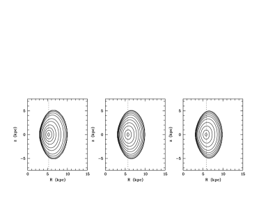
Figure 7: A plot of the spatial density in the meridional plane of models with $r_{\rm min}=3$ kpc, $r_{\rm max}=10$ kpc, $\alpha=4$ and $\beta=4$ (left), 8 (middle) and 12 (right). The boundary of this region is given by equation 42, hence all models fill the same volume. The higher the value of $\beta$, the more the high-angular momentum orbits are populated. This causes the position of the peak density (marked by the dashed line) to slowly shift outwards.

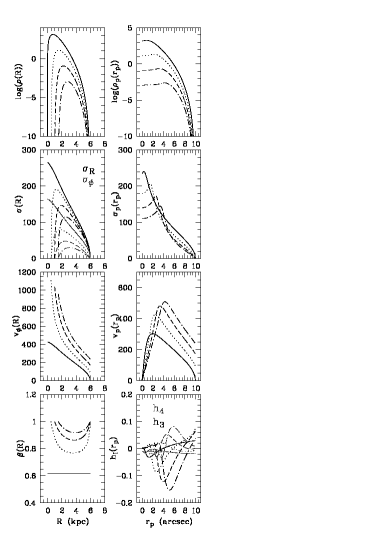
Figure 8: The influence of the angular momentum cut-off on the kinematics of models with $\alpha=6$, $\beta=2$, $r_{\rm max}=6$ kpc is demonstrated. The values of the inner radius are $r_{\rm min}=0$ kpc (solid line), 0.5 kpc (dotted line), 1.0 kpc (dashed line) and 1.5 kpc (dashed-dotted line). In the left column, a number of intrinsic kinematic quantities are plotted. The radius $R$ is measured in the equatorial plane, $z^{\prime}=0$. From top to bottom : the logarithm of the spatial luminosity density $\rho(R)$, the radial (black) and the tangential velocity dispersion (gray), the rotation velocity $v_{\phi}(R)$ and Binney’s anisotropy parameter $\beta(R)$. In the right column, the projected kinematics are presented. The radius $r_{p}$ lies along the long axis of the models. From top to bottom : the logarithm of the projected luminosity density $\rho_{p}(r_{p})$, the projected velocity dispersion $\sigma_{p}(r_{p})$, the projected streaming velocity $v_{p}(r_{p})$ and the Gauss-Hermite coefficients $h_{3}$ and $h_{4}$ (gray).

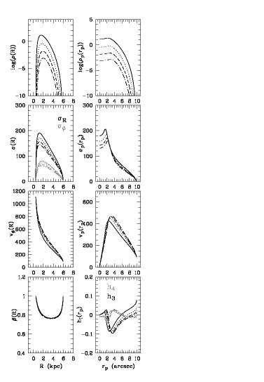
Figure 9: The influence of the parameter $\beta$ on the kinematics of models with $\alpha=6$, $r_{\rm min}=0.5$ kpc and $r_{\rm max}=6$ kpc is demonstrated. The values of $\beta$ are 2 (full line), 4 (dotted line), 6 (dashed line) and 8 (dashed-dotted line). In the left column, a number of intrinsic kinematic quantities are plotted. The radius $R$ is measured in the equatorial plane, $z^{\prime}=0$. From top to bottom : the logarithm of the spatial density $\rho(R)$, the radial (black) and the tangential velocity dispersion (gray), the rotation velocity $v_{\phi}(R)$ and Binney’s anisotropy parameter $\beta(R)$. In the right column, the projected kinematics are presented. The radius $r_{p}$ lies along the long axis of the models. From top to bottom : the logarithm of the projected density $\rho_{p}(r_{p})$, the projected velocity dispersion $\sigma_{p}(r_{p})$, the projected streaming velocity $v_{p}(r_{p})$ and the Gauss-Hermite coefficients $h_{3}$ (black) and $h_{4}$ (gray).

Mean velocity

For the mean rotation velocity, one finds

$$v_{\phi}(\varpi,z^{\prime}) = \frac{\mu_{0,1,0}(\varpi,z^{\prime})}{\rho(\varpi,z^{\prime})}$$ (43)

$$=\frac{L_{0}}{\varpi}+\frac{\beta+1}{\alpha+\beta+3}\left(\sqrt{\psi(r)-E_{0}}-\frac{L_{0}}{\sqrt{2}\varpi}\right)$$

$$\times\frac{\,{}_{2}F_{1}\left(-\alpha-1,\alpha+2;\alpha+\beta+4;\frac{\sqrt{2\varpi^{2}(\psi-E_{0})}-L_{0}}{2\sqrt{2\varpi^{2}(\psi-E_{0})}}\right)}{\,{}_{2}F_{1}\left(-\alpha-1,\alpha+2;\alpha+\beta+3;\frac{\sqrt{2\varpi^{2}(\psi-E_{0})}-L_{0}}{2\sqrt{2\varpi^{2}(\psi-E_{0})}}\right)}.$$

At the boundary of the component, the mean rotation velocity takes the value $v_{\phi}=L_{0}/\varpi=\sqrt{2(\psi(r)-E_{0})}$. The parameter $\beta$ has little impact on the rotation velocity profile, as shown in figure 8 and figure 9. The extreme values of the rotation velocity are determined solely by $L_{0}$ and $E_{0}$, making the rotation velocity a very sensitive function of these parameters.

Velocity dispersion

Since $l$ and $n$ are completely equivalent in equation (40), it is obvious that the velocity dispersions $\sigma^{2}_{\varpi}(\varpi,z^{\prime})$ and $\sigma^{2}_{z^{\prime}}(\varpi,z^{\prime})$ are always equal. This is the case for any model with a distribution function that depends only on $E$ and $L_{z^{\prime}}$. One finds that

$$\sigma^{2}_{\varpi}(\varpi,z^{\prime}) = \sigma^{2}_{z^{\prime}}(\varpi,z^{\prime})$$ (44)

$$=\frac{2}{\alpha+\beta+3}\sqrt{\psi(r)-E_{0}}\left(\sqrt{\psi(r)-E_{0}}-\frac{L_{0}}{\sqrt{2}\varpi}\right)$$

$$\times\frac{\,{}_{2}F_{1}\left(-\alpha-2,\alpha+3;\alpha+\beta+4;\frac{\sqrt{2\varpi^{2}(\psi-E_{0})}-L_{0}}{2\sqrt{2\varpi^{2}(\psi-E_{0})}}\right)}{\,{}_{2}F_{1}\left(-\alpha-1,\alpha+2;\alpha+\beta+3;\frac{\sqrt{2\varpi^{2}(\psi-E_{0})}-L_{0}}{2\sqrt{2\varpi^{2}(\psi-E_{0})}}\right)}$$

$$\sigma^{2}_{\phi}(\varpi,z^{\prime}) = 2\sum_{i=0}^{2}\frac{(\beta+1)_{i}}{(\alpha+\beta+3)_{i}}\left(\frac{L_{0}}{\sqrt{2}\varpi}\right)^{2-i}$$ (45)

$$\times\left(\sqrt{\psi(r)-E_{0}}-\frac{L_{0}}{\sqrt{2}\varpi}\right)^{i}$$

$$\times\frac{\,{}_{2}F_{1}\left(-\alpha-1,\alpha+2;\alpha+\beta+i+3;\frac{\sqrt{2\varpi^{2}(\psi-E_{0})}-L_{0}}{2\sqrt{2\varpi^{2}(\psi-E_{0})}}\right)}{\,{}_{2}F_{1}\left(-\alpha-1,\alpha+2;\alpha+\beta+3;\frac{\sqrt{2\varpi^{2}(\psi-E_{0})}-L_{0}}{2\sqrt{2\varpi^{2}(\psi-E_{0})}}\right)}$$

$$-v^{2}_{\phi}(\varpi,z^{\prime}).$$

Figures 8 and 9 also show that the anisotropy parameter $\beta_{\phi}$, with

$$\beta_{p}hi(\varpi,z^{\prime})=1-\frac{\sigma_{\phi}(\varpi,z^{\prime})}{\sigma_{\varpi}(\varpi,z^{\prime})}$$ (46)

is almost independent of the components parameter $\beta$ but very sensitive to the value of the angular momentum cutoff $L_{0}$.

4.3.4 The spatial line-of-sight velocity distribution

For the calculation of the spatial LOSVD, the DF will be directly integrated over the two velocity components in the plane of the sky. The integration over the line of sight will have to be performed numerically since it depends on the shape of the potential, which is generally only known numerically. We decompose the velocity vector in a component parallel to the line of sight, $v_{p}$, and two components in the plane of the sky, $v_{1}$ and $v_{2}$. The polar unit vector $\vec{e}_{\phi}$ can be written with respect to the vectors ($\vec{e}_{z},\vec{e}_{1},\vec{e}_{2}$) with $\vec{e}_{g}$ the unit vector along the line of sight and $\vec{e}_{1}$ and $\vec{e}_{2}$ unit vectors in the plane of the sky :

$$\vec{e}_{\phi}=b_{1}\vec{e}_{g}+b_{2}\vec{e}_{1}+b_{3}\vec{e}_{2},$$ (47)

with $b_{1}^{2}+b_{2}^{2}+b_{3}^{2}=1$. We now rewrite the distribution function as a function of $v_{p}$, $v_{1}$ and $v_{2}$ :

$$F(\varpi,z,v_{\varpi},v_{\phi},v_{z})\,dv_{\varpi}\,dv_{\phi}\,dv_{z}=F(\varpi,z,v_{p},v_{1},v_{2})\,dv_{p}\,dv_{1}\,dv_{2}$$ (48)

$$= \frac{\varpi^{n}}{2^{n/2}}\left(\psi-E_{0}-\frac{1}{2}(v_{p}^{2}+v_{1}^{2}+v_{2}^{2})\right)^{\alpha}$$

$$\times \left(i_{\rm rot}(b_{1}v_{p}+b_{2}v_{1}+b_{3}v_{2})-\frac{L_{0}}{\varpi}\right)^{n}\,dv_{p}\,dv_{1}\,dv_{2}.$$

Here and in the following, the power on the angular momentum will be assumed to be an integer, denoted by $n$. LOSVDs of components with non-integer values for this parameter will have to be calculated numerically. The velocity components in the plane of the sky, $v_{1}$ and $v_{2}$, can be expressed in polar coordinates $(v,\vartheta)$

$$v_{1} = v\cos\vartheta\hskip 30.00005ptv\geq 0,\,\,\vartheta\in[0,2\pi]$$

$$v_{2} = v\sin\vartheta.$$ (49)

Taking this transformation into account and introducing the notation

$$b_{2} = b\cos\chi\hskip 30.00005ptb\geq 0,\,\,\chi\in[0,2\pi]$$

$$b_{3} = b\sin\chi,$$ (50)

following expression can be obtained

$$F(\varpi,z,v,\vartheta,v_{p})\,dv_{p}v\,dv\,d\vartheta = \frac{\varpi^{n}}{2^{n/2}}\left(\psi-E_{0}-\frac{1}{2}(v_{p}^{2}+v^{2})\right)^{\alpha}$$ (51)

$$\times\left(i_{\rm rot}b_{1}v_{p}+bv\cos\vartheta-\frac{L_{0}}{\varpi}\right)^{n}\,dv_{p}v\,dv\,d\vartheta,$$

in which $\chi$ has been dropped, since the sign and the zero-point of $\vartheta$ are immaterial. The cosines $b$ and $b_{1}$ obey the relation $b^{2}+b_{1}^{2}=1$, with $b$ always positive. The distribution function has to be integrated over that part of the rectangle

$$0\leq v \leq\sqrt{2(\psi-E_{0})-v_{p}^{2}},$$

$$0\leq \vartheta \leq 2\pi$$ (52)

where

$$i_{\rm rot}b_{1}v_{p}+bv\cos\vartheta-\frac{L_{0}}{\varpi}\geq 0.$$ (53)

To relieve the notation throughout the remaining calculations, the following parameters will be used

$${\cal A} = \sqrt{2(\psi-E_{0})-v_{p}^{2}},$$

$${\cal P} = i_{\rm rot}b_{1}v_{p}-\frac{L_{0}}{\varpi},$$

$$\cos\vartheta_{0} = -\frac{{\cal P}}{{\cal A}b}.$$ (54)

The calculations will proceed along different paths depending on whether ${\cal P}\geq 0$ or ${\cal P}\leq 0$. The area in the rectangle (52) over which the distribution function has to be integrated is further limited by the positivity constraint on the angular momentum, (53). This translates in the extra constraints

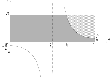
Figure 10: The grey shaded area in the $(v,\vartheta)$-plane marks the area over which the distribution function has to be integrated to calculate the spatial LOSVD if ${\cal P}\geq 0$. The hatched rectangle is defined by $0\leq v\leq\cal A$ and $0\leq\vartheta\leq\pi$. The integration area is bounded at the right by the curve $v\leq\frac{-\cal P}{b\cos\vartheta}$.

$$v \geq -\frac{{\cal P}}{b\cos\vartheta},\,\,\,\cos\vartheta\geq 0,$$

$$v \leq -\frac{{\cal P}}{b\cos\vartheta},\,\,\,\cos\vartheta\leq 0.$$ (55)

The spatial LOSVD can then be calculated as

$$\phi(\varpi,z^{\prime},v_{p}) = \frac{\varpi^{n}}{2^{\alpha+n/2}}\int_{0}^{{\cal A}^{2}}({\cal A}^{2}-v^{2})^{\alpha}dv^{2}$$ (56)

$$\times\int_{0}^{\pi}\left({\cal P}+bv\cos\vartheta\right)^{n}d\vartheta,$$

with the integration interval defined by (52) and (55).

${\cal P}\geq 0$

In this case, the distribution function has to be integrated over the grey shaded area in figure 10. Only if ${\cal P}<{\cal A}b$ will the second of the curves (55) intersect the rectangle (52).

${\cal P}\geq{\cal A}b\geq 0$

The $z^{\prime}$-component of the angular momentum is positive everywhere inside the rectangle (52). The integration over $\vartheta$ can be performed over the entire interval $[0,\pi]$, and so

$$\int_{0}^{\pi}\left({\cal P}+bv\cos\vartheta\right)^{n}d\vartheta =$$ (58)

$$\pi{\cal P}^{n}\,_{2}F_{1}\left(-\frac{n}{2},\frac{1-n}{2};1;\left(\frac{bv}{{\cal P}}\right)^{2}\right),$$

where $[n/2]$ is the largest integer, less or equal to $n/2$. Now, the integration over $v$ can be tackled. This integral reduces to a Beta-function and the spatial LOSVD can be written in the following elegant form :

$$\phi(\varpi,z^{\prime},v_{p}) = \frac{2\pi}{2^{n/2}}\frac{\varpi^{n}}{\alpha+1}\left(i_{\rm rot}b_{1}v_{p}-\frac{L_{0}}{\varpi}\right)^{n}$$ (59)

$$\times\left(\psi-E_{0}-\frac{v_{p}^{2}}{2}\right)^{\alpha+1}$$

$$\times_{2}F_{1}\left(-\frac{n}{2},\frac{1-n}{2};\alpha+2;\frac{b^{2}(2(\psi-E_{0})-v_{p}^{2})}{(i_{\rm rot}b_{1}v_{p}-\frac{L_{0}}{\varpi})^{2}}\right),$$

which is finite and well-behaved for all integer $n$ and real $\alpha$.

${\cal P}\leq{\cal A}b$

In this case, $\cos\vartheta_{0}\leq 0$ and $\vartheta_{0}\in[\frac{\pi}{2},\pi]$. The second of the curves defined by (55) cuts out a piece of the rectangle (52) and hence the distribution function has to be integrated over the shaded area in figure 10 :

$$\phi(\varpi,z^{\prime},v_{p}) = \frac{\varpi^{n}}{2^{\alpha+n/2}}\sum_{i=0}^{n}{n\choose i}{\cal P}^{n-i}b^{i}$$ (60)

$$\times\left(\int_{0}^{\vartheta_{0}}(\cos\vartheta)^{i}\,d\vartheta\underbrace{\int_{0}^{{\cal A}^{2}}(v^{2})^{i/2}({\cal A}^{2}-v^{2})^{\alpha}\,dv^{2}}_{\textstyle h_{1}}\right.$$

$$\left.+\int_{\vartheta_{0}}^{\pi}(\cos\vartheta)^{i}d\vartheta\underbrace{\int_{0}^{(\frac{\cal P}{b\cos\vartheta})^{2}}(v^{2})^{i/2}({\cal A}^{2}-v^{2})^{\alpha}\,dv^{2}}_{\textstyle h_{2}}\right).$$

The first auxiliary function $h_{1}$ is simply a Beta-function

$$h_{1} = {\cal A}^{2(\alpha+1)+i}B(\alpha+1,\frac{i}{2}+1).$$ (61)

The second function $h_{2}$ is an incomplete Beta-function and can be rewritten in terms of a hypergeometric function :

$$h_{2} = \frac{2{\cal A}^{2\alpha}}{2+i}\left(\frac{\cal P}{b\cos\vartheta}\right)^{i+2}$$ (62)

$$\times\,_{2}F_{1}\left(-\alpha,1+\frac{i}{2};2+\frac{i}{2};\left(\frac{\cal P}{{\cal A}b\cos\vartheta}\right)^{2}\right).$$

Thus, we obtain the following expression for the spatial LOSVD

$$\phi(\varpi,z^{\prime},v_{p})=$$ (63)

$$\frac{\Gamma(\alpha+1)}{2^{\alpha+n/2}}\varpi^{n}{\cal A}^{2(\alpha+1)}{\cal P}^{n}\sum_{i=0}^{n}{n\choose i}\frac{\Gamma(1+\frac{i}{2})}{\Gamma(\alpha+2+\frac{i}{2})}\left(\frac{{\cal A}b}{\cal P}\right)^{i}$$

$$\times\int_{0}^{\vartheta_{0}}(\cos\vartheta)^{i}\,d\vartheta+\frac{2\varpi^{n}}{2^{\alpha+n/2}}{\cal A}^{2\alpha}\frac{{\cal P}^{n+2}}{b^{2}}\sum_{i=0}^{n}\frac{1}{i+2}{n\choose i}$$

$$\times\sum_{k=0}^{\infty}\frac{(-\alpha)_{k}(1+i/2)_{k}}{k!(2+i/2)_{k}}\left(\frac{\cal P}{{\cal A}b}\right)^{2k}\int_{\vartheta_{0}}^{\pi}(\cos\vartheta)^{-2(k+1)}d\vartheta.$$

We first turn our attention to the second term of (63). Here, only negative odd powers of $\cos\vartheta$ appear in the integral. The integration can be done analytically with the aid of Gradshteyn & Ryzhik (1965) and yields the result :

$$\int_{\vartheta_{0}}^{\pi}(\cos\vartheta)^{-2(k+1)}d\vartheta =$$ (64)

$$-\frac{\sin\vartheta_{0}}{2k+1}\sum_{j=0}^{k}\frac{(-k)_{j}}{(\frac{1}{2}-k)_{j}}(\cos\vartheta_{0})^{2(j-k)-1}.$$

As to the first term of (63), the even and odd powers of $\cos\vartheta$ have to treated separately

$$\sum_{i=0}^{n}{n\choose i}\frac{\Gamma(1+\frac{i}{2})}{\Gamma(\alpha+2+\frac{i}{2})}\left(\frac{{\cal A}b}{\cal P}\right)^{i}\int_{0}^{\vartheta_{0}}(\cos\vartheta)^{i}\,d\vartheta$$ (65)

$$= \frac{\theta_{0}}{\Gamma(\alpha+2)}\,_{2}F_{1}\left(\frac{n}{2},\frac{1-n}{2};\alpha+2;\left(\frac{{\cal A}b}{\cal P}\right)^{2}\right)$$

$$\hskip 5.0pt+\sin\vartheta_{0}\sum_{j=0}^{n}\frac{(-n)_{j}}{\Gamma(j)}\frac{\Gamma(1+\frac{j}{2})}{\Gamma(\alpha+\frac{j}{2}+2)}\left(-\frac{{\cal A}b}{\cal P}\right)^{j}\times$$

$$\hskip 35.00005pt\sum_{l=0}^{[\frac{j-1}{2}]}\frac{((1-j)/2)_{l}}{(1-\frac{j}{2})_{l}}(\cos\vartheta_{0})^{j-2l-1}.$$

Thus, we are lead to the following expression for the spatial LOSVD:

$$\phi(\varpi,z^{\prime},v_{p})=$$ (66)

$$\frac{2\vartheta_{0}}{2^{n/2}}\frac{\varpi^{n}}{\alpha+1}\left(i_{\rm rot}b_{1}v_{p}-\frac{L_{0}}{\varpi}\right)^{n}\left(\psi-E_{0}-\frac{v_{p}^{2}}{2}\right)^{\alpha+1}$$

$$\times_{2}F_{1}\left(-\frac{n}{2},\frac{1-n}{2};\alpha+2;\frac{b^{2}(2(\psi-E_{0})-v_{p}^{2})}{(i_{\rm rot}b_{1}v_{p}-\frac{L_{0}}{\varpi})^{2}}\right)$$

$$+2\Gamma(\alpha+1)\sin\vartheta_{0}\frac{\varpi^{n}}{2^{n/2}}\left(\psi-E_{0}-\frac{v_{p}^{2}}{2}\right)^{\alpha+1}\left(i_{\rm rot}b_{1}v_{p}-\frac{L_{0}}{\varpi}\right)^{n}$$

$$\times\sum_{j=0}^{n}\frac{(-n)_{j}}{(j+1)!}\left(-\frac{{\cal A}b\cos\vartheta_{0}}{i_{\rm rot}b_{1}v_{p}-\frac{L_{0}}{\varpi}}\right)^{j}$$

$$\times\sum_{l=0}^{[\frac{j-1}{2}]}\frac{((1-j)/2)_{l}}{(1-\frac{j}{2})_{l}}(\cos\vartheta_{0})^{-2l-1}$$

$$-\tan\vartheta_{0}\frac{\varpi^{n}}{2^{n/2}}\frac{1}{b^{2}}\left(\psi-E_{0}-\frac{v_{p}^{2}}{2}\right)^{\alpha}\left(i_{\rm rot}b_{1}v_{p}-\frac{L_{0}}{\varpi}\right)^{n+2}$$

$$\times\sum_{i=0}^{n}\frac{1}{i+2}{n\choose i}$$

$$\times\sum_{k=0}^{\infty}\frac{(-\alpha)_{k}(1+\frac{i}{2})_{k}(\frac{1}{2})_{k}}{(\frac{3}{2})_{k}(2+\frac{i}{2})_{k}k!}\left(\frac{i_{\rm rot}b_{1}v_{p}-\frac{L_{0}}{\varpi}}{b\cos\vartheta_{0}\sqrt{2(\psi-E_{0})-v_{p}^{2}}}\right)^{2k}$$

$$\times\,_{2}F_{1}\left(-k,1;\frac{1}{2}-k;(\cos\vartheta_{0})^{2}\right).$$

In the limit ${\cal P}\rightarrow{\cal A}b$, one finds that $\vartheta_{0}\rightarrow\pi$ and the complicated expression (66) reduces to the far easier formula (59), as it should. The rather daunting formula (66) will only be well-behaved for integer values of $\alpha$ since then the last summation (with summation variable $k$) terminates after a finite number of terms.

${\cal P}<0$

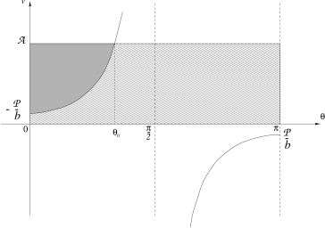
Figure 11: The grey shaded area in the $(v,\vartheta)$-plane marks the area over which the distribution function has to be integrated to calculate the spatial LOSVD in the case ${\cal P}<0$. The hatched rectangle is defined by $0\leq v\leq\cal A$ and $0\leq\vartheta\leq\pi$. The integration area is bounded by the curve $v\geq\frac{-\cal P}{b\cos\vartheta}$.

In this case, $\cos\vartheta_{0}=-\frac{\cal P}{{\cal A}b}>0$ and hence $\vartheta_{0}\in[0,\frac{\pi}{2}]$. The distribution function now has to be integrated over the shaded area in the $(v,\vartheta)$-plane presented in figure 11. Only if $|{\cal P}|<{\cal A}b$ will the first of the curves (55) intersect the rectangle (52).

$|{\cal P}|\geq{\cal A}b$

The integration area defined by the equations (55) and (52) vanishes, hence the spatial LOSVD is identically zero for all $|{\cal P}|\geq{\cal A}b$.

$|{\cal P}|<{\cal A}b$

The distribution function must be integrated over the grey shaded area in figure 11 :

$$\phi(\varpi,z^{\prime},v_{p})=$$ (67)

$$\frac{\varpi^{n}}{2^{\alpha+n/2}}\sum_{i=0}^{n}{n\choose i}{\cal P}^{n-i}b^{i}\int_{0}^{\vartheta_{0}}(\cos\vartheta)^{i}\,d\vartheta$$

$$\times\int_{(\frac{|\cal P|}{b\cos\vartheta})^{2}}^{{\cal A}^{2}}(v^{2})^{i/2}({\cal A}^{2}-v^{2})^{\alpha}\,dv^{2}.$$

We start with the integration over the velocity in the plane of the sky, $v$, which can be performed analogously to (61) and (62) :

$$\int_{(\frac{|\cal P|}{b\cos\vartheta})^{2}}^{{\cal A}^{2}}(v^{2})^{i/2}({\cal A}^{2}-v^{2})^{\alpha}\,dv^{2}$$ (68)

$$= {\cal A}^{2(\alpha+1)+i}B(\alpha+1,\frac{i}{2}+1)$$

$$-\frac{2}{i+2}\left(\frac{|\cal P|}{b\cos\vartheta}\right)^{i+2}{\cal A}^{2\alpha}$$

$$\times\,_{2}F_{1}\left(-\alpha,\frac{i}{2}+1;\frac{i}{2}+2;\left(\frac{|\cal P|}{{\cal A}b\cos\vartheta}\right)^{2}\right).$$

Thus, we obtain an expression that is almost exactly like (63)

$$\phi(\varpi,z^{\prime},v_{p})=$$ (69)

$$\frac{\Gamma(\alpha+1)}{2^{\alpha+n/2}}\varpi^{n}{\cal A}^{2(\alpha+1)}{\cal P}^{n}$$

$$\times\sum_{i=0}^{n}{n\choose i}\frac{\Gamma(1+\frac{i}{2})}{\Gamma(\alpha+2+\frac{i}{2})}\left(\frac{{\cal A}b}{\cal P}\right)^{i}\int_{0}^{\vartheta_{0}}(\cos\vartheta)^{i}\,d\vartheta$$

$$-\frac{2\varpi^{n}}{2^{\alpha+n/2}}{\cal A}^{2\alpha}\frac{{\cal P}^{n+2}}{b^{2}}\sum_{i=0}^{n}\frac{(-1)^{i}}{i+2}{n\choose i}$$

$$\times\sum_{k=0}^{\infty}\frac{(-\alpha)_{k}(1+i/2)_{k}}{k!(2+i/2)_{k}}\left(\frac{\cal P}{{\cal A}b}\right)^{2k}\int_{0}^{\vartheta_{0}}(\cos\vartheta)^{-2(k+1)}d\vartheta.$$

The integrations over $\vartheta$ are handled analogously to (64) and (65) and we finally obtain

$$\phi(\varpi,z^{\prime},v_{p})=$$ (70)

$$\frac{2\vartheta_{0}}{2^{n/2}}\frac{\varpi^{n}}{\alpha+1}\left(i_{\rm rot}b_{1}v_{p}-\frac{L_{0}}{\varpi}\right)^{n}\left(\psi-E_{0}-\frac{v_{p}^{2}}{2}\right)^{\alpha+1}$$

$$\times_{2}F_{1}\left(-\frac{n}{2},\frac{1-n}{2};\alpha+2;\frac{b^{2}(2(\psi-E_{0})-v_{p}^{2})}{(i_{\rm rot}b_{1}v_{p}-\frac{L_{0}}{\varpi})^{2}}\right)$$

$$+2\Gamma(\alpha+1)\sin\vartheta_{0}\frac{\varpi^{n}}{2^{n/2}}\left(\psi-E_{0}-\frac{v_{p}^{2}}{2}\right)^{\alpha+1}$$

$$\times\left(i_{\rm rot}b_{1}v_{p}-\frac{L_{0}}{\varpi}\right)^{n}$$

$$\times\sum_{j=0}^{n}\frac{(-n)_{j}}{(j+1)!}\left(\frac{{\cal A}b\cos\vartheta_{0}}{|i_{\rm rot}b_{1}v_{p}-\frac{L_{0}}{\varpi}|}\right)^{j}$$

$$\times\sum_{l=0}^{[\frac{j-1}{2}]}\frac{((1-j)/2)_{l}}{(1-\frac{j}{2})_{l}}(\cos\vartheta_{0})^{-2l-1}$$

$$-\tan\vartheta_{0}\frac{\varpi^{n}}{2^{n/2}}\frac{1}{b^{2}}\left(\psi-E_{0}-\frac{v_{p}^{2}}{2}\right)^{\alpha}\left(i_{\rm rot}b_{1}v_{p}-\frac{L_{0}}{\varpi}\right)^{n+2}$$

$$\times\sum_{i=0}^{n}\frac{(-1)^{i}}{i+2}{n\choose i}$$

$$\times\sum_{k=0}^{\infty}\frac{(-\alpha)_{k}(1+\frac{i}{2})_{k}(\frac{1}{2})_{k}}{(\frac{3}{2})_{k}(2+\frac{i}{2})_{k}k!}\left(\frac{i_{\rm rot}b_{1}v_{p}-\frac{L_{0}}{\varpi}}{b\cos\vartheta_{0}\sqrt{2(\psi-E_{0})-v_{p}^{2}}}\right)^{2k}$$

$$\times\,_{2}F_{1}\left(-k,1;\frac{1}{2}-k;(\cos\vartheta_{0})^{2}\right).$$

This formula will only be used for integer values of $\alpha$, as discussed in the case of (66). In the limit $|{\cal P}|\rightarrow{\cal A}b$, $\vartheta_{0}$ vanishes. The spatial LOSVD becomes identically zero and remains zero for all $|{\cal P}|\geq{\cal A}b$.

5 Dynamical model

The two most prominent absorption lines of the Ca II triplet were used as input for the modelling. The spectra were rebinned to reach sufficiently high S/N. The S/N was about 50 at radii less than 10 ^′′ and from these spectra 182 points were included in the fit. For larger radii, the S/N was about 30 and only 91 points per spectrum were included in the fit.

5.1 Potential

The observed R-band surface brightness profile was deprojected into a spherical luminosity density. Assuming a mass-to-light ratio, this lead to a mass density that was used to calculate a potential by means of the Poisson equation. A model with constant M/L did not result in a satisfactory fit. Hence, a number of models with a dark matter halo were considered. For all these models, the dark halo component was added in the form of a spherical distribution of mass, where the amount of matter is increasing as a power of the radius. Different models have different fractions of total matter mass to light emitting mass at a chosen radius (here 2 kpc or $0.9r_{e}$, this radius is only for scaling and has no physical meaning) and different total masses. In this way, a grid of models was created, and the smallest value for $\chi^{2}$ was taken to be indicative for the best matching potential.

The best results were obtained with a potential where the spatial density of the total amount of matter was 2.5 times the spatial density of the amount of luminous matter within 2 kpc. This scaling implies that the total mass within $1r_{e}$ is $1.6\times 10^{11}M_{\odot}$, 70 $\%$ of which is luminous matter. The total mass at $2r_{e}$ is $5\times 10^{11}M_{\odot}$, and 37 $\%$ of this is luminous matter (see also upper panel in figure 12). Figure 12 (lower panel) shows the total mass profile in solid line in comparison with the luminous matter mass profile in dashed line.

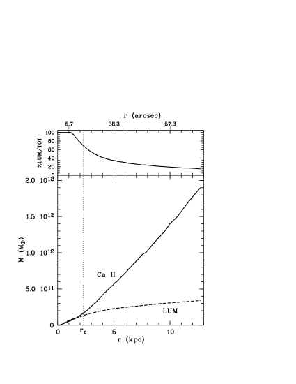
Figure 12: In the lower panel: Mass profile for the best fitting model based on the Ca II triplet feature (solid line) and for the best fitting model without dark matter (dashed line). In the upper panel: the fraction of luminous matter relative to all matter for the best fitting models with dark matter.

It was not necessary to include a central black hole in the model to obtain a good fit for the central spectra.

5.2 Dynamical model

The model that best fits the spectra around the two most prominent Ca II triplet lines, at 8542 Å and 8662 Å, is shown in figure 13. From these plots, no obvious shortcoming of the model can be indicated.

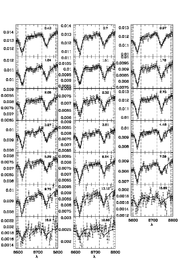
Figure 13: Data and model around the two strongest Ca II triplet lines. The regions included in the fit are located between the intervals indicated by dashed lines and with centre around 8620 Å and 8750 Å. The projected radius of the positions where the spectra are taken are indicated in the panels.

Figure 14 shows some derived quantities of the model. The upper left panel shows the projected density on major and minor axis. As can be seen, the flattening of the galaxy is well reproduced. The right panels show calculated projected mean velocity and velocity dispersion profiles (solid lines), together with uncertainties on these quantities as derived from the model. The values and error estimates for the projected mean velocity $\langle v_{p}\rangle$ and velocity dispersion $\sigma_{p}$, presented in 2.4, are plotted on top in dots. In figure 14 also the anisotropy parameters $\beta_{\phi}=1-(\sigma^{2}_{\phi}/\sigma^{2}_{r})$ (in solid line) and $\beta_{\theta}=1-(\sigma^{2}_{\theta}/\sigma^{2}_{r})$ (in dotted line) are displayed in the lower left panel. The parameter $\beta_{\phi}$, Binney’s anisotropy parameter, is close to zero for the central parts, indicating an isotropic DF there, becomes slightly posivite for intermediate radii and slightly negative for radii larger than 2 kpc, indicating that the model is tangentially anisotropic there.

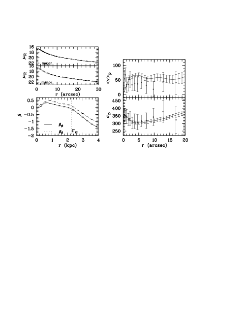
Figure 14: Some derived moments from the model. Left column: projected density on major and minor axis and the anisotropy parameters $\beta_{\phi}$ and $\beta_{\theta}$. Right column: projected mean velocity and projected velocity dispersion.

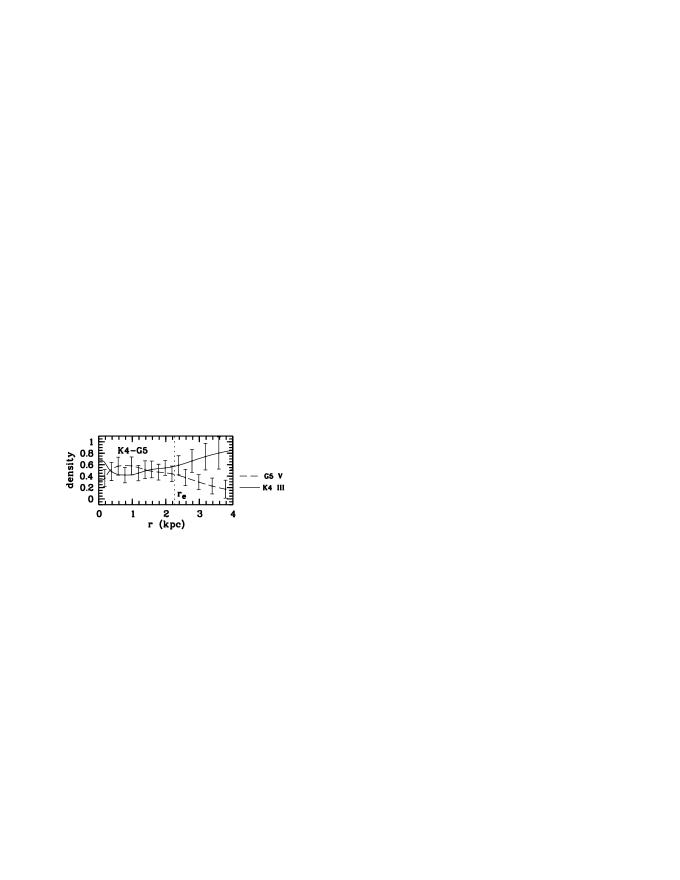
Figure 15: Template mixes for the best model based on the two strongest lines of the Ca II triplet.

A mix of G5V and K4III stars gives the best fit to the spectra in this wavelength range. The value for $\chi^{2}$ obtained for the fit is 2267, the second best model has a $\chi^{2}$ of 2383. The resulting template mix of this best model can be found figure 15. The relative densities are calculated from the spatial number densities of the model.

More models, with other template mixes, than shown here were calculated. The results mainly confirm the trends seen in figure 15. In the model with K4III and G2V stars e.g., the contribution of G2V stars to the density is larger than the G5V stars in the K4III-G5V panel, but the same radial behaviour occurs.

6 Discussion

If a model is strongly tangential in the outer regions, most of the motion occurs along the line of sight and this may increase the projected velocity dispersion. Hence, the influence of dark matter may be underestimated. This is the strongest argument for including the fourth order shape parameter of the observed LOSVD as input parameter in a dynamical model, because it is believed to indicate whether a lot of orbits are observed near their tangent point or not. For the calculation of this dynamical model, we did not rely on the extracted LOSVD nor the derived kinematic parameters, but on the observed spectra.

The dynamical model is slightly tangentially anisotropic from roughly $1r_{e}$ on, as can be seen in figure 14.

Tangential anisotropy in the outer regions of the model is also seen in other models for e.g. NGC 3377 (Gebhardt et al., 2000), NGC 1023 (Bower et al, 2001) and also in the sample modeled by Kronawitter et al. (2000).

Estimating kinematic parameters through a dynamical model clearly reduces the amount of scatter in the kinematic profile, as is illustrated in figure 14 (right panels). This is easily understood since the model induces additional dynamical constraints on the parameters and as a result the values of the parameters taken at different radii are not independent. When the parameters are inferred directly from the observed spectra, there is no connection between the parameters at different radii.

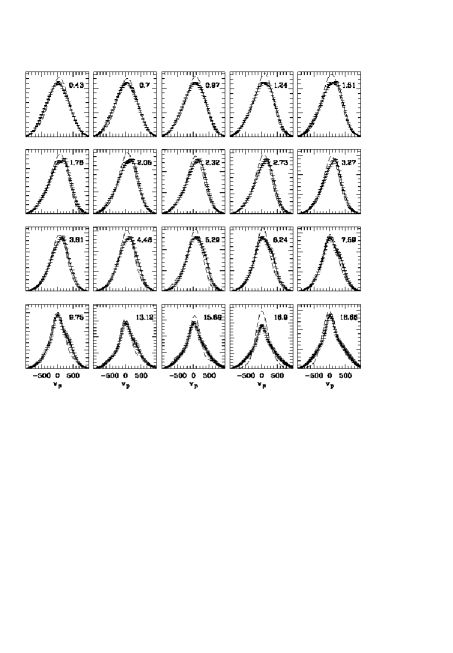
Figure 16: LOSVDs as reconstructed from the kinematic parameters presented in 2.4 (dashed line) and calculated from the model (solid line). Also error bars are calculated from the model. The radii at which the LOSVDs are taken are indicated in arcsec in the panels.

Figure 16 presents LOSVDs as derived from the observations and the model. The profiles calculated from the kinematic parameters presented in 2.4 are shown in dashed lines, the solid lines present the LOSVDs with error bars calculated from the model. It is clear that the LOSVDs calculated from the kinematic parameters all have an approximately Gaussian shape. This is of course due to the parametrization that is used to present them. The LOSVDs calculated from the model show a large variety of shapes. Some of these profiles cannot be reproduced by a Gauss-Hermite series truncated at fourth order (or even sixth order) and hence a perfect agreement with the LOSVDs calculated from the kinematic parameters cannot be expected.

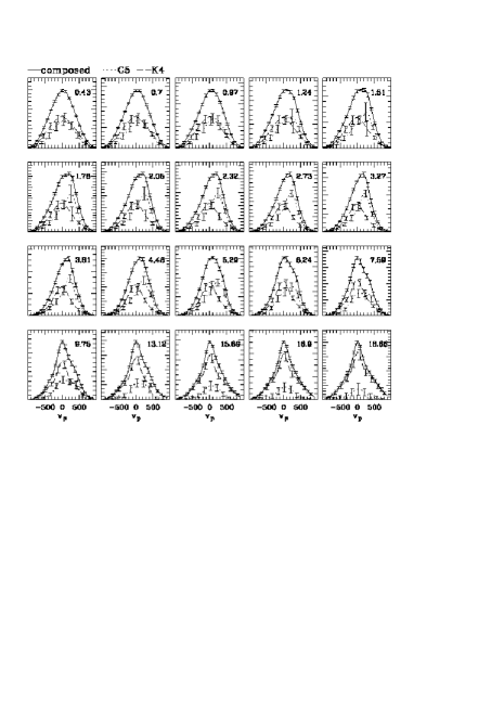
Figure 17: LOSVDs calculated from the model: for the composed DF in full lines, for the G5V population in dotted lines and for the K4III population in dashed lines. The different radii at which the LOSVDs are taken are indicated in arcsec in the panels.

The shapes of the LOSVDs calculated from the model can be better understood when looking at figure 17. In this figure the LOSVDs for the different stellar populations, together with the composed LOSVD (solid lines) are shown. The relative height of the LOSVDs for the two populations is in agreement with the information in figure 15. A full discussion of the role of the stellar populations will be deferred to a subsequent paper, where a fit will be presented that takes into account 2 wavelength regions.

Instead of comparing full profiles, one could argue in favor of comparing their most relevant parameters. Unfortunately, this is not a trivial exercise. The mathematical elegane of the Hermite expansion lies in the fact that it forms an orthogonal series, with coefficients that can be calculated by integrals that follow from the theory. However, this is almost never the way the Hermite coefficients are calculated in practice: they are generally determined with some kind of minimization after performing a convolution. This causes the loss of the orthogonality property. This becomes clear in an exercise where a stellar template spectrum convolved with a LOSVD with parameters $-20\rm{km/s}<\langle v\rangle<20\rm{km/s}$, $\sigma=300\rm{km/s}$ , $h_{3}=0$, $h_{4}=0$, $h_{5}=0$ and $h_{6}=0.1$ is analysed in the same way as real galactic spectra and kinematic parameters up to $h_{4}$ are determined. Since the template spectrum used to create this synthetic spectrum is equal to the one used to determine the parameters again, there is no influence of continuum subtraction or template mismatch on the results. The synthetic galaxy spectrum has a S/N of 130 in the centre and the light profile follows a de Vaucouleurs that resembles the light profile of NGC 3258. The result of this simulation is shown in figure 18. The values retrieved for $\langle v\rangle$ and $h_{3}$ correspond to the original values. On the other hand, the values for $\sigma$ and $h_{4}$ are clearly higher than the values of the input LOSVDs.

This indicates that the kinematic parameters as derived from a Gauss-Hermite parametrization are in practice not independent, in the sense that power in the higher orders than considered in the expansion may contaminate lower order parameters. In the case of $h_{4}$ this can give rise to wrong conclusions concerning the anisotropy in the stellar motion. Naively, one could conclude that it is better to go to higher order than $h_{4}$ in the parametrization. Unfortunately, the signal-to-noise ratio in outer regions of a galaxy is hardly sufficient to derive reliable values for $h_{4}$, so it does not make sense to try to determine higher order parameters. The useful information in LOSVDs derived from observations is thus very limited, due to the rather low signal-to-noise of the observations. Therefore, though it is a good idea to use a parametrization with a limited number of parameters to represent these LOSVD, there is, as a consequence, also only a limited number of shapes for LOSVDs possible, as extracted from these observations. This on top of the fact that these parameters are not independent, which means that caution should be taken when interpreting them. On the other hand, LOSVDs calculated from dynamical models can have a much larger variety of shapes. It would be unfair to reject model LOSVDs because they do not match the ones that are derived from observations, simply because the information in LOSVDs derived from spectra is very limited, while the dynamical models offer much more freedom.

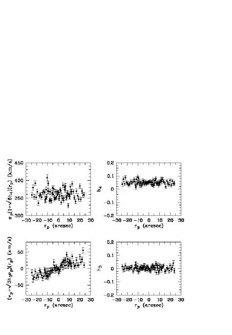
Figure 18: Result from a simulation where $\langle v\rangle$, $\sigma$, $h_{3}$ and $h_{4}$ are determined from spectra that are a convolution of LOSVDs with $-20\rm{km/s}<\langle v\rangle<20\rm{km/s}$, $\sigma=300\rm{km/s}$, $h_{3}=h_{4}=h_{5}=0$ and $h_{6}=0.1$.

7 Conclusions

In this paper we use a method to analyse spectra from elliptical galaxies in order to retrieve dynamical information and to perform a stellar population synthesis at the same time. The method originates from the field of dynamical modelling and is presented by DD98. The main idea is that the different stellar populations that contribute to the integrated galaxy spectrum do not necessarily share the same kinematic characteristics. Hence, in terms of dynamical modelling, they should be given different distribution functions. This paper reports for the first time on the application of our modelling technique to data. The attention is focused on the presentation of the method and on establishing a mass estimate for the galaxy under study. A second paper will discuss the possibilities for stellar population studies and will go deeper into the distribution functions for separate stellar templates.

Modelling the spectra directly yields an estimate for the total amount of mass, and an analysis of the internal dynamics of the galaxy. This technique, using galaxy spectra as input data, also differs from more traditional modelling strategies that rely on kinematic parameters that are derived from the spectra in the sense that a two step process is turned into a one step process, thereby coming closer to the astrophysical issues.

Photometric and spectroscopic observations for NGC 3258 are presented. This galaxy has almost perfect elliptical isophotes, and has an effective radius of $12.95^{\prime\prime}$ (2.26 kpc). Images in B and R show a slightly off-centre nucleus. There seems to be a slight reddening of the nucleus. The photometry also reveals the presence of a central dust disk (0.17 kpc - 0.26 kpc). The R band photometry was used to derive a spherical potential for the luminous matter.

The photometry, together with galaxy spectra containing dynamical information up to $1.3r_{e}$ are combined into a dynamical model. The best dynamical model for NGC 3258 is the one with a dark matter halo that contributes 30% of the total mass at $1r_{e}$ and 63% of the total mass at $2r_{e}$. From $1.45r_{e}$ outwards, the model is dominated by dark matter. The total mass within $1r_{e}$ is $1.6\times 10^{11}M_{\odot}$ and $(M/L)_{R}\approx 65$, $(M/L)_{R}\approx 30$, whereas the total mass extrapolating to $2r_{e}$ is $5\times 10^{11}M_{\odot}$ and $(M/L)_{R}\approx 95$,$(M/L)_{B}\approx 43.5$. In the region without dark matter $(M/L)_{R}\approx 14$ ($(M/L)_{B}\approx 6.4$). The modelling did not require to include a central black hole.

The anisotropy parameter (see figure 14) indicates that the model is isotropic in the centre, is radially anisotropic between 0.2 and 2 kpc (i.e. within $1r_{e}$) and becomes slightly tangentially anisotropic further out.

A simulation has shown that for the analysis of LOSVDs derived from observations by means of a truncated Gauss-Hermite series, power in higher orders than considered in the expansion may contaminate lower order parameters. This is a worrysome result, since $h_{4}$ profiles derived from observations tend to be interpreted in terms of anisotropy of the galaxy. If this parameter is contaminated by power in higher orders by some form of aliasing induced by the fitting process, this may lead to an erroneous interpretation or at least may make comparison of $h_{4}$’s obtained by different methods problematic. Moreover, due to the freedom in the dynamical model, one cannot expect that LOSVDs calculated from a dynamical model as presented in this paper can be approximated by Gauss-Hermite series that are truncated at a low order.

8 Acknowledgments

VDB acknowledges financial support from FWO-Vlaanderen. WWZ acknowledges the support of the Austrian Science Fund (project P14783) and the support of the Bundesministerium für Bildung, Wissenschaft und Kultur.

This research has made use of the NASA/IPAC Extragalactic Database (NED) which is operated by the Jet Propulsion Laboratory, California Institute of Technology, under contract with the National Aeronautics and Space Administration.

References

- Bettoni & Buson, (1987) Bettoni D., Buson L.M., 1987, A&AS, 67, 341
- Bower et al (2001) Bower G.A., Green R.F., Bender R., Gebhardt K., Lauer T.R., Magorrian J., Richstone D.O., Danks A., Gull T., Hutchings J., Joseph C., Kaiser M. E., Weistrop D., Woodgate B., Nelson C., Malumuth E.M., 2001, ApJ, 550, 75.
- Bregman et al. (1998) Bregman J.N., Snider B.A., Grego L., Cox C.V., 1998, ApJ, 499, 670
- Carter et al., (1999) Carter D., Bridges T.J., Hau G.K.T., 1999, MNRAS, 307, 131
- Ciotti et al., (1995) Ciotti et al., 1995, MNRAS, 276, 961
- De Bruyne et al., (2001) De Bruyne V., Dejonghe H., Pizzella A., Bernardi M., Zeilinger W.W., 2001, ApJ, 546, 903
- De Bruyne et al., (2003) De Bruyne V., Vauterin P., De Rijcke S., Dejonghe H., 2003, MNRAS, 339, 215
- Dejonghe, (1989) Dejonghe H., 1989, ApJ, 343, 113
- Dejonghe & De Bruyne, (2003) Dejonghe H., De Bruyne V., ’From observations to distribution function’, in Lecture Notes in Physics ’Galaxies and Chaos. Theory and Observations’, Springer Verlag
- De Rijcke & Dejonghe (1998) De Rijcke S., Dejonghe H., 1989, MNRAS, 298, 677 (DD98)
- De Rijcke et al. (2003) De Rijcke S., Dejonghe H., Zeilinger W.W., Hau G.K.T., 2003, A&A, 400, 119
- Fabiano et al. (1992) Fabbiano G., Kim D.-W., Trinchieri G., 1992, ApJS, 80, 531
- Ferrarese & Merritt (2000) Ferrarese L., Merritt D., 2000, ApJ, 539, L9
- Ferrari et al. (2002) Ferrari F., Pastoriza M.G., Macchetto F.D., Bonatto C., Panagia N., Sparks W.B., 2002, A&A, 389, 355
- Fisher et al., (1995) Fisher D., Franx M., Illingworth G., 1995, ApJ, 448, 119
- Gebhardt et al. (2000) Gebhardt K., Richstone D., Kormendy J., Lauer T. R., Ajhar E.A., Bender R., Dressler A., Faber S. M., Grillmair C., Magorrian J., Tremaine S., 2000, AJ, 119, 1157
- Gerhard et al. (1998) Gerhard O., Jeske G., Saglia R.P., Bender R., 1998, MNRAS, 295, 197
- Gradshteyn & Ryzhik (1965) Gradshteyn I.S., Ryzhik I.M., Table of integrals, series and products, 1965, Academic Press, New York&London
- Jenkins (1983) Jenkins C.R., 1983, MNRAS, 205, 1321
- Joseph et al. (2001) Joseph, C.L., Merritt D., Olling R., Valluri M., Bender R., Bower G., Danks A., Gull T., Hutchiongs J., Kaiser M.E., Maran S., Weistrop D., Woodgate B., Malumuth E., Nelson C., Plait P., Lindler D., 2001, ApJ, 550, 668
- Koprolin & Zeilinger (2000) Koprolin W., Zeilinger W.W., 2000, A&AS, 145, 71
- Kronawitter et al. (2000) Kronawitter A., Saglia R.P., Gerhard O., Bender R., 2000, A&AS, 144, 53
- Pellegrini et al. (1997) Pellegrini S., Held E.V., Ciotti L., 1997, MNRAS, 288, 1
- Sadler et al. (1989) Sadler E.M., Jenkins C. R., Kotanyi C.G., 1989, MNRAS, 240, 591
- van der Marel (1994) van der Marel R. P., 1994, MNRAS, 270, 271
- van der Marel & Franx (1993) van der Marel R. P., Franx M., 1993, ApJ, 407, 525