Constraints on Quasar Continuum, BELR, and BALR Physics from SDSS Composite Spectra

Abstract

We review recent results on quasars from the SDSS as they relate to our understanding of the UV/optical continuum, the broad emission line region, and the broad absorption line region. The ensemble average colors of large numbers of quasars promise to provide constraints on the optical/UV continuum emission mechanism. High-ionization emission-line blueshifts and emission line properties as a function of optical/UV spectral index trace the structure of the broad emission line region. Statistical analysis of the broad absorption line quasar population suggests that they are more ubiquitous than one might otherwise think and are not likely to represent a completely distinct population of quasars, but that the BAL trough properties are a function of the underlying optical continuum and emission properties of the quasar.

Princeton University Observatory, Princeton, NJ 08544-1001

Princeton University Observatory, Princeton, NJ 08544-1001 and Departamento de Astronomía y Astrofísica, Facultad de Física, Pontificia Universidad Católica de Chile, Casilla 306, Santiago 22, Chile

Johns Hopkins University, Department of Physics and Astronomy, 3400 N. Charles St., Baltimore, MD 21218

Univ. of Pittsburgh, Dept. of Physics and Astronomy, 3941 O’Hara St., Pittsburgh, PA 15260

The Pennsylvania State University, Department of Astronomy and Astrophysics, 525 Davey Lab, University Park, PA 16802

Princeton University Observatory, Princeton, NJ 08544-1001

1. The Optical/UV Continuum

In the rest-frame optical and UV, after accounting for emission lines, quasars are reasonably well-described by a power-law continuum with a typical spectral index of $\alpha_{\nu}\sim-0.3$–$0.5$ (e.g., Francis et al. 1991; Vanden Berk et al. 2001).

Using data from Sloan Digital Sky Survey (SDSS; York et al. 2003) quasars (Richards et al. 2002a), we find that the spread in the color distribution as measured by SDSS quasars is roughly $\Delta\alpha_{\nu}=\pm 0.25$ ($1\sigma$) and is formally resolved (Richards et al. 2003). That is, the width of the distribution is much broader than the errors. Detailed analysis of the contributions of dust extinction (which is the most likely cause of the red tail in Figure 1; Hall et al. 2004a, this volume) and variability (Wilhite et al. 2004, this volume) are needed in order to accurately describe the intrinsic continua of quasars; however, the raw data already provide constraints for accretion disk models. We can confirm that the average color is significantly redder than is expected from a simplistic accretion disk modeled as a sum of blackbodies ($\alpha_{\nu}=1/3$; e.g., Shakura & Sunyaev 1973; Hubeny et al. 2000), but the bluest quasars can be even bluer than $\alpha_{\nu}=1/3$. Comparisons of the distribution of colors to accretion disk models will provide an important constraint on those models (e.g., Blaes 2004, this volume).

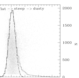
Figure 1.: Distribution of relative $g-i$ colors (observed colors corrected by the median color as a function of redshift) for the SDSS DR1 quasar sample. Note the red tail that extends beyond an otherwise Gaussian distribution. (Adapted from Richards et al. 2003.)

2. Broad Emission Line Region

The SDSS data can help improve our understanding of the broad emission line region (BELR) by studying the changes in the strengths and profiles of the broad emission lines as a function of their rest-frame optical/UV colors and as a function of the well-known blueshift of high-ionization emission lines (especially C IV) with respect to low-ionization and forbidden, narrow emission lines (Gaskell 1982; Richards et al. 2002b).

The SDSS data reveal that that blueshift of C IV may be caused by a lack of flux in the red wing rather than by a bulk blueward shift of the line since the blueshifted lines are also systematically weaker — perhaps due to an orientation and/or radiative transfer effect in a disk-wind (e.g., Chiang & Murray 1996). Although the composites in Figure 2 are normalized by redshift and luminosity, the fact that the blueshifted composites have weaker C IV emission suggests that the emission line blueshifts and the Baldwin (1977) Effect have the same physical basis. See Francis & Koratkar (1995) for confirmation of this relationship in another sample of quasars. Not correcting redshifts for these blueshifts may be the reason that SPCA analyses (Shang & Wills 2004, this volume; Yip et al. 2004, this volume) find a Baldwin Effect in the apparent line cores rather than the red wing of the line; see Vanden Berk et al. (2004, this volume) for supporting evidence. Furthermore, how well one can measure the mass of a quasar from its C IV profile clearly depends on the exact nature of these blueshifts (c.f., Vestergaard 2004a, this volume; Warner, Hamann, & Dietrich 2004, this volume).

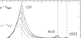
Figure 2.: Composite spectra as a function of the redshift difference between CIV and MgII. (Adapted from Richards et al. 2002b.)

Figure 3.: Selected emission line regions of composite spectra of the reddest (solid line) and bluest (dashed line) SDSS quasars [excluding those that appear dust reddened]. (Adapted from Richards et al. 2003.)

We also find that quasar emission lines are a function of the optical/UV continuum slope (i.e., color). Figure 3 shows major emission line regions for composite spectra constructed from quasars with bluer and redder than average relative $g-i$ colors (Richards et al. 2003). More work needs to be done to understand this relationship, but it is clear that these differences are not (solely) due to the redder quasars (those denoted ‘steep’ in Fig. 1) having more dust.

3. Broad Absorption Line Region

The SDSS quasar survey has already provided the largest sample to date of broad absorption line quasars. The most significant results are as follows. The balnicity index (Weymann et al. 1991) distribution increases steeply with decreasing absorption strength (Tolea, Krolik, & Tsvetanov 2003; Reichard et al. 2003a), which suggests that the true population of quasars with intrinsic absorption outflows is larger than is generally thought and also that quasars with wide high-velocity outflows may not be distinct from those with narrower low-velocity outflows. Analysis of the continuum and emission line regions of SDSS BALQSOs by Reichard et al. (2003b) suggests that the optically selected BALQSO sample is drawn from the same parent population as the nonBALQSO sample, but it does appear that the properties of BALQSOs (terminal velocity, ionization state, etc.) are not independent of the intrinsic color and emission line properties. Thus even though BALQSOs may not be a distinct population, certain types of quasars may be more likely to host certain kinds of BALs. For example, composites of intrinsically red and intrinsically blue BALQSOs (after correction for dust reddening) appear to have somewhat different broad absorption trough properties; see Figure 4.

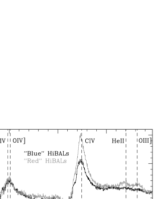
Figure 4.: Composite spectra of HiBALs with intrinsically blue spectral indices (black line) and intrinsically red spectral indices (grey line). Each composite is the average of 41 quasars. (Adapted from Reichard et al. 2003.)

4. Support for a Hybrid Model?

We suggest that the combination of the results from SDSS BALQSOs above and previous results (such as the difference between narrow absorption in flat- and steep-spectrum radio-loud quasars) lends support to a model where the disk-wind ranges from being nearly polar to nearly equatorial (with BAL or BAL-like outflows existing in all objects); see Figure 5. Such a scenario might result from a hybrid model which combines MHD and line-driven (LD) radiation pressure such as discussed by both Proga (2003) and Everett (2003). If this were the case, the Elvis (2000) picture (with polar NAL absorption regions and more equatorial BAL absorption regions; Figure 5, top) might be seen as being the ensemble average picture, rather than the picture of an individual quasar. Elvis (2000) discusses similar scenarios in relation to incorporating radio-loud quasars into the picture and how luminosity might affect the opening angle of the wind. Such a picture would create two orientation effects (the opening angle of the wind and the tilt of the disk) that may be difficult to disentangle; however such a scenario would open up some freedom to explain all known classes of AGN using a disk-wind model.

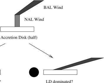
Figure 5.: Absorption line data suggests that quasars may all have BAL-like outflows, but that their properties depend on the opening angle of the wind which may range from equatorial to polar (perhaps depending on the relative strength of the disk magnetic fields and radiation pressure).

Acknowledgments.

Funding for the creation and distribution of the SDSS Archive (http://www.sdss.org/) has been provided by the Alfred P. Sloan Foundation, the Participating Institutions, the National Aeronautics and Space Administration, the National Science Foundation, the U.S. Department of Energy, the Japanese Monbukagakusho, and the Max Planck Society.

The SDSS is managed by the Astrophysical Research Consortium (ARC) for the Participating Institutions. The Participating Institutions are The University of Chicago, Fermilab, the Institute for Advanced Study, the Japan Participation Group, The Johns Hopkins University, Los Alamos National Laboratory, the Max-Planck-Institute for Astronomy (MPIA), the Max-Planck-Institute for Astrophysics (MPA), New Mexico State University, University of Pittsburgh, Princeton University, the United States Naval Observatory, and the University of Washington.

References

Baldwin, J. A. 1977, ApJ, 214, 679

Chiang, J. & Murray, N. 1996, ApJ, 466, 704

Elvis, M. 2000, ApJ, 545, 63

Everett, J. E. 2003, astro-ph/0212421

Francis, P. J., et al. 1991, ApJ, 373, 465

Francis, P. J., & Koratkar, A. 1995, MNRAS, 274, 504

Gaskell, C .M. 1982, ApJ, 263, 79

Hubeny, I., et al. 2000, ApJ, 533, 710

Proga, D. 2003, ApJ, 585, 406

Reichard, T. A., et al. 2003a, AJ, 125, 1711

Reichard, T. A., et al. 2003b, AJ, in press

Richards, G. T., et al. 2002a, AJ, 123, 2945

Richards, G. T., et al. 2002b, AJ, 124, 1

Richards, G. T., et al. 2003, AJ, 126, 1131

Shakura, N. I., & Sunyaev, R. A. 1973, A&A, 24, 337

Tolea, A., Krolik, J. H., & Tsvetanov, Z. 2002, ApJ, 578, 31

Vanden Berk, D. E., et al. 2001, AJ, 122, 549

Weymann, R. J., Morris, S. L., Foltz, C. B., & Hewett, P. C. 1991, ApJ, 373, 23

York, D. G., et al. 2000, AJ, 120, 1579

Discussion

Antonucci: How much of the spread in colors do you think is due to variability of individual objects as they vary in luminosity?

Richards: Variability certainly contributes significantly to the spread, but it is not the dominant factor. We estimate that it contributes about $0.05$ (out of $\sim 0.12$) to the $1\sigma$ spread in color (or about $0.1$ of $0.25$ in $\Delta\alpha$).