Galaxy luminosity evolution: how much is due to a model choice?

The cluster and field luminosity functions (LFs) determined on large homogeneous samples ($N>2200$ galaxies each) are almost indistinguishable, down to $M^{*}+4$ in the $r$ and $i$ filters, hence suggesting that the effect of the cluster environment on the galaxy properties does not affect the galaxy luminosity function in red bands. The similarity of the red band LFs in different environments suggests that the galaxy mass function is preserved during the galaxy infall in the cluster. By analyzing a large sample of galaxies in clusters, ideal from many points of view (multicolor data, large size, many clusters, metric magnitudes) we found that luminosity evolution is required by the data but the latter do not unambiguously derive its flavour if a differential luminosity evolution between bright and faint galaxies is allowed. We show that the LF parameters (slope, characteristic magnitude and their evolution) and errors depend on assumptions in a way seldom recognized in literature. We also point out logical inconsistencies between hypothesis assumed in deriving literature LF and presented results, suggesting caution in interpreting similar published results.

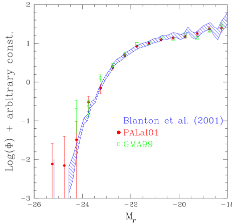
Figure 1: Luminosity function in the Gunn $r$ (left panel) and $i$ (right panel) for the cluster and field environments. The shaded area is the field LF derived by Blanton et al. (2001), green open and close red points mark GMA99 and PALal01 LFs, respectively. GMA99 do not compute any $i$ band LF using pseudo–total magnitudes.

1 Introduction

The study of the cluster luminosity function (LF) has at least two immediate objectives: to look for environmental related effects, as remarked by possible differences between the cluster and field LF, and to look for galaxy evolution, by comparing the LF at different redshifts. Both the objectives are considered in this paper.

At the present date, cluster and field LFs of large samples of galaxies in the nearby universe ($z<0.25$) have been computed (Garilli, Maccagni & Andreon 1999, hereafter GMA99; Blanton et al. 2001; Paolillo, Andreon, Longo et al. 2001, hereafter PALal01; Norberg et al. 2002b; de Propris et al. 2003). A convergence on the field LF, absent just few years ago (GMA99, see their figure 10) seems to be reached (Norberg et al. 2002b), in spite of an initial disagreement (Blanton et al. 2001) between Sloan Digital Sky Survey (SDSS) and 2 degree Field Galaxy Redshift Survey (2dFGRS) LFs. A convergence on the cluster LF, when the considered sample is large enough to dump out possible vagaries of individual cluster LF, seems also reached, given the good agreement between the GMA99 LF, based on 65 clusters, the PAal01 LF, computed for 39 clusters, and older LFs (see GMA99 and PALal01 for details). There are, however, recent cluster LFs that systematically differ from all LFs published thus far (e.g. Goto et al. 2002).

Given the reached convergence on the field and cluster LFs, it is therefore time to compare them.

LFs are usually characterized by a Schechter (1976) function:

$$\phi(M)=\phi^{*}10^{0.4(\alpha+1)(M^{*}_{0}-M)}e^{-10^{0.4(M^{*}-M)}}$$

where $M^{*}$ and $\alpha$ are the characteristic magnitudes and the slope of the function, respectively. $\phi^{*}$ is a normalization parameter not relevant in this work.

For the field environment, the evolution of the LF, i.e the $z$ dependence of the best fit parameters of the LF, has been explored. Lin et al. (1999) presented some evidence for an evolution on $M^{*}$ in the redshift range $0.12<z<0.55$, of the order of 0.4 (0.3) mag in the rest–frame $B$ ($R$) over the explored redshift range. Very recently, Blanton et al. (2003) analysis of a larger SDSS data set found a similar variation for $M^{*}$ in the redshift range $0.02<z<0.22$ in $g^{\prime},r^{\prime},i^{\prime}$. Blanton et al. (2003) and Lin et al. (1999), both claim evolution assuming a not evolving LF shape.

For the clusters, evolution of the LF is, instead, much less explored. GMA99 found only marginal, if any, evidence for evolution in the redshift range $0.05<z<0.25$ by binning cluster LFs in two $z$ ranges. de Propris et al. (1999) found evolution on $M^{*}$ in the $K$ band in the $0.2<z<0.9$ redshift range for $M<M^{*}+1$ galaxies and assuming that $\alpha$ does not evolve with $z$.

In this paper we have a twofold objective: first to compare the cluster and field LFs (§2), second to measure the evolution of the cluster LF using the same formalism used for measuring the evolution of the field LF. The data and the analysis is summarized in §3, whereas results are presented in Section 4.

We adopt $H_{0}=50$ km s^-1 Mpc^-1 and $\Omega=1$. However, the $H_{0}$ value reduce off in the comparisons, and is, therefore, irrelevant. Furthermore, the considered samples are at low redshift.

2 Cluster and field LF

The comparison of the cluster and field LF have been attempted several times in literature (for example Bromley et al. 1998a,b; Christlein 2000; Balogh et al. 2001; Valotto et al. 1997; Trentham & Hodgkin 2002), with opposite claims about the LF environmental dependence.

Figure 1 shows three luminosity functions in the Gunn $r$ and $i$ bands of the largest and most homogeneous samples measured thus far. Green open points mark the GMA99 cluster $r$ band LF. It has been obtained in the Gunn $r$ filter for about 2200 galaxies in 65 clusters, ranging in redshift from 0.05 to 0.25. Red closed points mark the PALal01 $r$ and $i$ band LFs. The LFs have been obtained by using $F$ and $N$ photographic plates calibrated in the $r$ and $i$ Gunn photometric system. The sample is about 1.5 time larger than the GMA99 one and is drawn from 39 clusters in the redshift range $0.06<z<0.28$. The two cluster LFs shown in Figure 1 are derived using different materials (CCD vs photographic plates), different ways to subtract interloper galaxies (using colors vs using control fields), different definitions of “total” magnitude, different portions of the clusters (GMA99 explored only the center, whereas PALal01 considered the whole cluster), and finally, the absolute limiting magnitude is approximately independent on $z$ for GMA99, whereas it is systematically brighter for more distant clusters in PALal01. Although some clusters are in common between the two works, only a very minor fraction of galaxies are in common, because of the different depths and field of views of the two works. Therefore, the two LFs are really independent each other, and should not share common biases introduced by the data analysis (that is completely different in the two works).

The dashed area in Figure 1 show the $r^{\prime}$ and $i^{\prime}$ field LF, as measured by the SDSS (Blanton et al. 2001). The sample is larger than both previous samples by a factor of few (at most), and it extends over a similar redshift range: $0.02<z<0.17-0.20$. SDSS $r^{\prime}$ and $i^{\prime}$ filters are quite similar to the Gunn $r$ and $i$ filters, at least for galaxies at low redshift, because they map the emission coming from almost identical part of the galaxy spectrum. The major difference between the two systems is the star that defines the objects of zero magnitude (and color). In fact, for $r$ and $i$ filters, the conversion from SDSS to Gunn is almost independent on the object spectra (see Table 3 in Fukugita et al. 1995). We therefore correct the SDSS $r^{\prime}$ and $i^{\prime}$ SDSS magnitudes for the change of the zero mag standard star by using the values listed in Fukugita et al. (1995). Galaxies having a surface brightness profile following a de Vaucouleurs (1948) law have a Petrosian flux that underestimates by 0.1-0.2 mag the total mag (Blanton et al. 2001). Since most of the galaxies in cluster are early–type galaxies, and hence have a de Vaucouleurs (1948) radial profile, we made SDSS Petrosian magnitudes brighter by 0.15 mag, in order to make them comparable to “total” magnitudes derived in GMA99 (SExtractor (Bertin & Arnouts (1996) isophotal corrected magnitudes) and in PALal01 (Focas (Jarvis & Tyson 1981) “total” magnitudes). Finally, SDSS absolute magnitudes are corrected to our value of $H_{0}$. The vertical normalization of the LFs is arbitrary.

The three LFs are almost indistinguishable, hence suggesting that the effect of the cluster environment on the galaxy properties does not affect the galaxy luminosity function in red filters. The comparison performed by de Propris et al. (2003) between cluster and field $B_{j}$ LF shows instead differences in the cluster and field blue LF. The similarity of the luminosity function in different environments in the red bands suggests that the galaxy mass function is preserved during the galaxy infall in the cluster, whereas the blue luminosity, more sensitive to star bursts, is altered.

The found similarity of the LF in different environments seems at variance with previous (opposite) findings.

– Many LF determinations (e.g. Small, Sargent & Hamilton 1997; Bromley et al. 1998b; Christlein 2000; Balogh et al. 2001) use Sandage, Tammann & Yahil (1979, STY) and Efstathiou, Ellis & Peterson (1988, EEP) LF estimators, in which the spatial dependent part of the LF factors out under the assumption of an LF universality. These works claim to have measured different LFs in different environments, in spite of having assumed that the LF does not depend on environment in the LF computation. Hypothesis and results are, therefore, in direct contradiction. Furthermore, according to Efstathiou, Ellis & Peterson (1988), STY and EEP estimators underestimate errors if the LF universality does not hold. Because of the logical inconsistency between hypothesis and conclusions, we consider the results of these papers as suggestive at most, and with underestimated errors.

We also note that the skewed (Blanton et al. 2001) LF of the Las Campanas Redshift Survey undermines the claims of environmental effects based on that survey, such as Christlein (2000), Bromley et al. (1998b) and Balogh et al. (2001) results. Furthermore, Balogh et al. (2001) uses the 2MASS photometry (Jarrett et al. 2000), criticized by Andreon (2002a) because 2MASS misses dim galaxies and the outer halos of normal galaxies, hence giving skewed LFs, as confirmed by Blanton et al. (2003) and Bell et al. (2003).

– Cluster and field are found sometime to have different LFs. Some examples are shown in Valotto et al. (1997) and Zabludoff & Mulchaey (2000). Almost none of the papers comparing cluster and field LFs uses homogeneous and large samples as the ones used in this paper (see de Propris et al. 2003 as an exception), and none in the red bands considered in the present paper. Furthermore, only recently (Norberg et al. 2002b) there has been a convergence on the field LF. Therefore, the results of previous cluster vs field LF comparisons largely rely on which field LF has been considered. Just as an example in red bands, Zabludoff & Mulchaey (2000) do find differences between the LF of poor groups and the field when they adopt for the field the Lin et al. (1996) LF. The latter LF differ systematically from the SDSS LF for the reasons described in Blanton et al. (2001). The Zabludoff & Mulchaey (2000) result does not tell us about environmental differences, but about the slow convergence of the field LF to the present day determination.

The similarity of the global red LFs in different environments is not in contradiction with the suggested universality of the LFs of morphological types in the blue band (Sandage, Binggeli, & Tammann 1985; Jerjen & Tammann 1997; Andreon 1998). First, the LF of the types are measured in filters different from the ones studied in this paper. Second, the simplest interpretation of the suggested universality of the LFs of the morphological types is that galaxies change neither type nor luminosity. However, the same data can be interpreted as galaxies change type and luminosity, preserving at the same time the blue LFs of morphological types and the global mass function. Such an interpretations allows both the blue LF of the morphological types and the global red LF to be universal. It naturally allows the blue LF of cluster and field to be different, as observed by de Propris et al. (2003). Independently of the correct interpretation of the observations, the measure of the global mass function, here approximated by the red LF, is important in order to know whether galaxies change their mass during the infall in the cluster. Our present measure suggests that mass is preserved, at least in a statistical sense.

We caution the reader not to compare the SDSS and PALal01 $g$ band LFs, since the latter LF, although being internally consistent, is in a photometric system that can be linked to the standard SDSS $g^{\prime}$ system in a quite complicate way. We are now re-deriving the blue cluster LF, for a twice larger sample, in its “natural” system (i.e. in the $B_{J}$) (Paolillo et al. 2004).

A technical detail should now be mentioned. All three LFs shown in Figure 1 are derived assuming that luminosity evolution in the studied redshift range is negligible. Since all three LFs considered almost the same redshift range, the comparison makes sense even in the presence of luminosity evolution in the studied redshift range. In that case, the derived LFs are computed at the median $z$, which is almost the same for the three LFs ($0.15,0.12,0.10$ for GMA99, PALal01 and Blanton et al. 2001, respectively). Although this point is quite technical, this is an important one: the measured LF depends on the model used in its derivations, as shown in Section 4. Our comparison uses LFs derived adopting the same model.

3 Cluster LF evolution: data and analysis

In order to measure the LF evolution we use the sample presented in Garilli et al. (1996) and whose LFs have been previously presented in GMA99. This sample is ideal for such evolutionary study for several reasons. First, because all clusters are sampled at $M^{*}+3$ to $M^{*}+4$ independently on redshift (see GMA99 figure 5). The sample depth allows to measure the evolution of both $M^{*}$ and $\alpha$ at all studied redshifts, for the first time. Second, the fact that both $M^{*}$ and $\alpha$ can be measured at all studied redshifts should clarify the usual degeneracy between the two parameters and makes the results less sensitive to mis–interpretations. Third, GMA99 compute aperture magnitudes fixed in the galaxy frame (they use a 20 kpc aperture), magnitude that we adopted here. Such a metric aperture does not suffer the problem of isophotal magnitudes, or even pseudo–total one according to Dalcanton (1998), that bias the LF with $z$ in such a way to mimic evolution. The choice of a metric aperture is therefore essential. However, LFs derived with such an aperture are tilted with respect to the one computed using pseudo–total magnitudes, and the former cannot be compared to the latter. For this reason in Figure 1 we plot the GMA99 LF derived using pseudo–total magnitudes and not the one computed using aperture magnitudes. Fourth, three colors (Gunn $g$, $r$ and $i$) photometry is available, allowing to study the wavelength dependence of the possible evolution.

The only difference with GMA99 sample is that we discarded one cluster (MS0013+1558), because the studied part of it includes just one single galaxy. We remind that absolute magnitudes are k–corrected assuming an elliptical spectrum, with k–corrections taken from Frei & Gunn (1994).

We compute the LF using standard maximum–likelihood methods (STY, EEP) used for the field LF determination.

Given a sample of N galaxies in M clusters at redshift $z_{1},z_{2},...,z_{M}$, we compute the likelihood $L$ by the formula:

$$\ln L=\sum_{clusters}\sum_{galaxies}p_{i}$$

where $p_{i}$ is the individual conditional probability

$$p_{i}=p(M_{i}|z_{i})=\frac{\phi(M_{i})}{\int\phi(M)dM}$$

where the integral is evaluated over the range $[-\infty,mag_{lim}]$, where $mag_{lim}$ is the limiting magnitude, and where $\phi$ is the Schechter (1976) function modified for allowing $\alpha$ and $M^{*}$ to vary with $z$:

$$\phi(M)=\phi^{*}10^{0.4(\alpha_{z}+1)(M^{*}_{z}-M)}e^{-10^{0.4(M^{*}_{z}-M)}}$$

$$\alpha_{z}=\alpha_{0}-Pz$$

$$M^{*}_{z}=M^{*}_{0}-Qz$$

We hence take $M^{*}$ and $\alpha$ to vary linearly with $z$ with a rate given by $Q$, and $P$, respectively. Positive values for $P$ and $Q$ mean that in the past galaxies were brighter and the LF was steeper. Our $Q$ has the same meaning of $Q$ in Lin et al. (1999) and Blanton et al. (2003). Instead, their $P$ parameter has a different meaning from our $P$: we model the $\alpha$ evolution, whereas they model the $\phi^{*}$ evolution.

Best fit parameters are derived by maximizing the likelihood. Error ellipses in the ($M^{*},\alpha$) or ($P,Q$) planes are computed by finding the contour corresponding to

$$lnL=lnL-\frac{1}{2}\Delta\chi^{2}$$

where $\Delta\chi^{2}$ is the change in $\chi^{2}$ appropriate for the desired confidence level and a $\chi^{2}$ distribution (with two degree of freedom/interesting parameters for confidence contours, and one degree of freedom for single parameters).

The computation of the LF parameters by using the maximum likelihood method has a great advantage: the $\phi^{*}_{i}$ parameters (one per cluster) cancel out in computing $p_{i}$ (see the $p_{i}$ equation), and the dimension of the overall space to be explored decreases from 68 to 4.

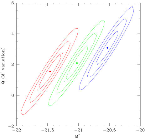
Figure 2: Confidence contours at the 68.3, 95.4 and 99.73 % confidence levels for two degree of freedom for $M^{*}$ and $Q=\partial M^{*}/\partial z$ when $\alpha$ is not allowed to evolve. The no–evolution locus is given by $Q=0$. For a passive evolving population $Q\sim 1.1-1.2$. $g$, $r$ and $i$ contours are in blue, green and red (also right to left).

4 Genuine evolution or built-in the LF model?

In literature, LFs have been computed under one of these three hypothesis:

– no evolution at all ($P=Q=0$). Only a few selected studies do not make such an assumption.

– no evolution on the LF slope ($P=0$) and an assumed evolution on $M^{*}$. This hypothesis is used by the 2dFGRS LF (Norberg et al. 2002b).

– no evolution on the LF slope ($P=0$). $M^{*}$ evolution ($Q$) is solved during the LF determination (CNOC LF, Lin et al. 1999; SDSS LF, Blanton et al. 2003)

We determine the cluster LF under all these hypothesis (and even more). Table 1 presents the derived best fit values and their errors. We will show that results, for the very same data sample, depend on the model used to derive the LF, i.e. on assumptions about $P$ and $Q$. In particular, best fit parameters and their error, luminosity evolution, and its statistical significance, all depend on the adopted model, suggesting caution in interpreting similar published results.

4.1 The usual case, i.e. assuming $P=Q=0$

By fixing $P=Q=0$, i.e. assuming no evolution at all, we found the same best fit ($M^{*},\alpha$) parameters found in GMA99, comfortably showing that the present algorithm converges to the same value previously found with an algorithm using the $\chi^{2}$. Presently and previously computed confidence contours also almost perfectly overlap each other. $M^{*}$ and $\alpha$ are correlated, and the correlation is shown in Figure 6 of GMA99.

We check for a possible incompleteness in the data sample, by computing the LF adopting half a magnitude brighter limiting magnitude in $r$: the newly determined best fit parameters are within the 68 % confidence level of the previous ones (i.e. the difference is less than 1/$\sqrt{2}$ combined $\sigma$), in agreement with independent checks done in GMA99.

The parameters just settled (i.e. $P=Q=0$) is the original Blanton et al. (2001) choice for the first SDSS LF derivation, and also the standard setting adopted in most LF derivations, such as the Stromlo–APM LF (Loveday et al. 1992), SSRS2 LF(da Costa et al. 1994), the CfA1 and CfA2 LF (Marzke et al. 1994), the Century Survey LF (Geller et al. 1997) the Corona Borealis LF (Small et al. 1997) the ESP LF (Zucca et al. 1997) and the K20 LF (Pozzetti et al. 2003).

4.2 $P=0$ and $\alpha$ fixed at the best global fit

Let now $Q$ to be free (i.e. we allow $M^{*}$ to evolve), and $\alpha$ to be fixed (i.e. $P=0$) at its best global fit. This setting is the same adopted in the Lin et al. (1999) LF determination. Blanton et al. (2003) in their second SDSS LF derivation do not use a Schechter function, but the sum of Gaussians, with fixed (i.e. not evolving) relative amplitude. Therefore, also in Blanton et al. (2003) the LF shape (slope) is not allowed to be redshift dependent.

Figure 2 shows confidence contours for $M^{*}$ and $\alpha$ for our sample. As expected, the present computed $M^{*}$ differs from the one computed in the previous section, by $Q\times z_{median}$, as it occurs between the first and second SDSS LF derivations (Blanton et al. 2003), the latter being different from the former “almost entirely because of the inclusion of evolution in the luminosity function model” (Blanton et al. 2003).

$Q$ turn out to be positive, i.e. galaxies are brighter in the past, in the three filters. $Q=0$ is ruled out at $\sim$90 to 99.73 % confidence level in the $g$ filter only, and therefore the statistical significance of the evidence is $\sim$2 to 3 $\sigma$ at most.

For an old passive evolving stellar population, $Q=1.1-1.2$ at the redshifts sampled in this work. Such values can easily derived from the convolution of the GISSEL96 (Bruzual & Charlot 1993) spectral energy distributions at the look back times sampled in the present work (i.e. $z<0.25$) with the Gunn filters. Best fit $Q$ values (2.1 and 3.1, see Table 1) derived by imposing a not evolving $\alpha$ are twice/three times larger than expected by assuming a passive luminosity evolution, $Q=1.1-1.2$, but compatible with them at the 68.3 (or better) % confidence level (see Figure 2).

If we stop our analysis here we would claim to have found evidence of luminosity evolution at $\sim$2 to 3 $\sigma$, in good agreement with Blanton et al. (2003), because our and their $Q$ values agree to better than $1\sigma$. Instead, we proceed further.

4.3 $Q$ forced to be as model predictions

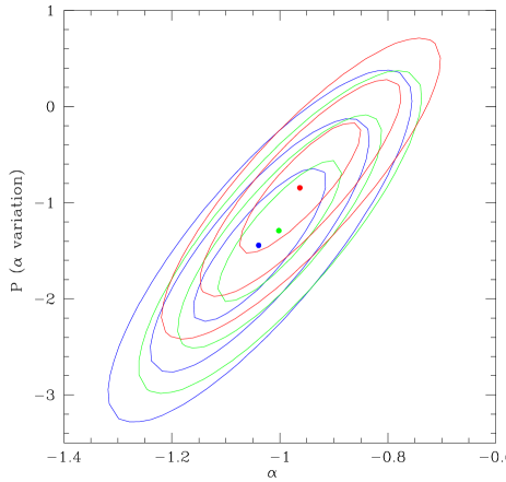
Figure 3: Confidence contours at the 68.3, 95.4 and 99.73 % confidence levels for two degree of freedom, for $\alpha$ and $P=\partial\alpha/\partial z$. $M^{*}$ is forced to passively evolve. $g$, $r$ and $i$ contours are in blue, green and red (also bottom to top).

We now assume that $Q$ is forced to be equal to the model prediction, i.e. $Q=1.1-1.2$ depending on filter, and $\alpha$ free to evolve. Figure 3 shows confidence contours for $P$ and $\alpha$. The best fit $P$ (i.e. the $\alpha$ derivative) is $\sim-1$ to $-1.5$, although $P\neq 0$ can be rejected at only the $\sim 95$ % confidence level (Figure 3). Therefore, $\alpha$ variations are suggested by the data but not required (evidence is $\sim 2\sigma$), if passive evolution is assumed.

With the further constraint of a fixed $\alpha$, this type of fit would make resemblance to the 2dFRS LF model (Norberg et al. 2002b), that assumes an evolution well reproduced by simple synthesis population models, and a unique (redshift independent) slope. Of course, being $M^{*}$ evolution imposed ab initio, it cannot independently derived by the LF analysis. At most, one may claim that the found luminosity evolution is compatible with the assumed one.

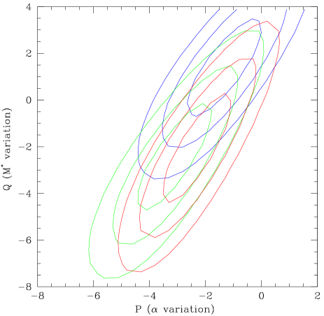
Figure 4: Confidence contours at the 68.3, 95.4 and 99.73 % confidence levels for two degree of freedom, for $P=\partial\alpha/\partial z$ and $Q=\partial M^{*}/\partial z$ when both $\alpha$ and $M^{*}$ are allowed to evolve. $r$, $i$ and $g$ contours are in green, red and blue (also, left to right). The no–evolution locus is given by $P=Q=0$. The passive evolving locus has $Q\sim 1.1-1.2$.

4.4 All parameters free

Let now $P$ and $Q$ to be free, in order to look for evolution in both the parameters. We do not force a priori that some of the parameters do not evolve with redshift, but we left them to evolve as the data allow. At difference of previous sections (and previous works, including SDSS and 2dFRS ones), in absence of a better knowledge we do not make a debatable assumption, and we allow all our parameters to be redshift dependent, as much as allowed by the data. We are here explicitly allowing bright and faint galaxies to evolve differently, as it is likely, because brighter galaxies tend to be redder and are therefore presumed to be older and slowly evolving.

Figure 3 shows $P,Q$ confidence contours for the three filters. The $P=Q=0$ point, i.e. the no–evolution case, is well outside the 99.73 % confidence contours in $g$ and $r$, whereas falls on the top of the 99.73 % confidence contours in the $i$ band. Therefore, unevolving $\alpha$ and $M^{*}$ are rejected at 3, or more, $\sigma$ in all three filters. Therefore, evolution is required by the data, although it is not by adopting the other LF considered models.

The point $Q\sim 1.15$ and $P=0$, i.e. the pure passive evolution expectation, is included in the 95.4 percent confidence contour in $g$ and $i$ and in the 99.73 percent confidence contour in $r$. Therefore, the passive evolution case is a statistically acceptable description of the data at 2 to 3 $\sigma$. Pure passive evolution, however, is not the unique solution allowed by the data. There are other acceptable solutions at $Q\sim 1.15$ (i.e. $M^{*}$ is passively evolving): a detailed inspection of Figure 3 shown that all the range $-3\la P\la 0$ is as good as (or better than) $P=0$. We remind that negative values for $P$ imply that the LF becomes flatter at higher redshift.

By leaving all parameter free, $M^{*}$ evolution is smaller, or even with opposite sign, than by keeping $\alpha$ fixed (see Table 1). Therefore, one more degree of freedom of evolution drastically influences the derived $M^{*}$ evolution. Such a degree of freedom is allowed by none of previous LF determinations, including 2dFRS and SDSS. Therefore, we warn the reader that other similar studies in literature, all of which assume a fixed and not evolving $\alpha$, may mis–interpret the found $M^{*}$ evolution.

By leaving all parameter free, errors on $M^{*}$ and $\alpha$ are larger (by a factor $\sim 3$) than when $P=Q=0$, i.e. under the usual hypothesis done in the LF computation, and are twice larger than when $\alpha$ is kept fixed.

In order to check that the flattening is not due to an increasing incompleteness at faint magnitudes with increasing redshift, we re–computed the best fit parameters considering only the galaxies at least half a magnitude brighter than the claimed completeness magnitude. We found almost identical best fit values (see Table 1 where we list results for the $r$ filter). A couple of clusters, mainly nearby, have deeper observation than the other clusters. In order to make the limiting magnitude even more uniform with redshift, we recomputed the best fit parameters by adopting the brighter between the claimed magnitude limits and $M_{r}=-17.5$ mag. We found identical best fit values and errors (see Table 1), as expected because only an handful of galaxies, out more than 2000, are removed by this cut. Therefore, best fit values and confidence contours are robust to incompleteness.

Table 1: Best fit parameters derived for different models

filter	$M^{*}$	$\alpha$	$Q\equiv\partial M^{*}/\partial z$	$P\equiv\partial\alpha/\partial z$	Notes
no evolution ($Q=P=0$)
$r$	$-21.38\pm 0.08$	$-0.84\pm 0.04$	(0)	(0)
$g$	$-21.08\pm 0.08$	$-0.88\pm 0.04$	(0)	(0)
$i$	$-21.72\pm 0.07$	$-0.85\pm 0.04$	(0)	(0)
$r$	$-21.40\pm 0.08$	$-0.88\pm 0.04$	(0)	(0)	$mag_{lim}$ half mag brighter
$\alpha$ fixed, i.e. Evolution on $M^{*}$ only ($P=0$)					see also Fig. 2
$r$	$-21.02\pm 0.11$	(-0.82)	$2.1\pm 0.7$	(0)
$g$	$-20.53\pm 0.11$	(-0.83)	$3.1\pm 0.8$	(0)
$i$	$-21.46\pm 0.12$	(-0.84)	$1.5\pm 0.8$	(0)
$M^{*}$ passive evolving, and evolution on $\alpha$ only ($Q=0$)					see also Fig. 3
$r$	$-21.15$	$-1.00\pm 0.08$	(1.15)	$-1.3\pm 0.6$
$g$	$-20.84$	$-1.04\pm 0.08$	(1.20)	$-1.4\pm 0.6$
$i$	$-21.51$	$-0.96\pm 0.08$	(1.10)	$-0.8\pm 0.6$
$M^{*}$ fixed, i.e. Evolution on $\alpha$ only ($Q=0$)
$r$	$-21.01$	$-1.13\pm 0.11$	(0)	$-2.1\pm 0.7$
$g$	$-20.53$	$-0.83\pm 0.11$	(0)	$3.1\pm 0.8$
$i$	$-21.46$	$-0.84\pm 0.12$	(0)	$3.1\pm 0.8$
$P$ and $Q$ free, i.e. evolution on both $M^{*}$ & $\alpha$					see also Fig. 4
$r$	$-21.71\pm 0.26$	$-1.27\pm 0.13$	$-2.4\pm 1.5$	$-3.1\pm 0.9$
$g$	$-20.79\pm 0.23$	$-1.02\pm 0.14$	$1.4\pm 1.4$	$-1.3\pm 0.9$
$i$	$-22.00\pm 0.26$	$-1.18\pm 0.13$	$-2.0\pm 1.6$	$-2.3\pm 0.9$
$r$	$-21.67\pm 0.28$	$-1.24\pm 0.15$	$-2.1\pm 1.7$	$-2.7\pm 1.6$	$mag_{lim}$ half mag brighter
$r$	$-21.71\pm 0.27$	$-1.28\pm 0.14$	$-2.5\pm 1.5$	$-3.2\pm 0.9$	$max(mag_{lim},-17.5)$

All tabulated errors are 1 $\sigma$ one–parameter errors. See Figures for two–parameters error contours. Fixed parameters are indicated in parenthesis.

4.5 $P=Q=0$ vs the correct solution when the LF evolves

Using the very same data, GMA99 split the sample in two redshift bins and derived the composed LF assuming no evolution inside each redshift bin ($\delta z\sim 0.1$). This is the standard way in which the evolution of the luminosity function is computed (e.g. Lilly et al. 1995; Ellis et al. 1996; Heyl et al. 1997; Cohen et al. 2002). The comparison of the LFs in the two redshift bins, performed using a $\chi^{2}$ approach, showed no statistically significant differences. In the present paper, by adopting a model in which $\alpha$ do not evolve, we found an evidence of evolution on $M^{*}$ at 2 to 3 $\sigma$. A model that allow both $M^{*}$ and $\alpha$ to evolve excludes the no–evolution case at better than 3 $\sigma$.

The analysis presented here supersedes the comparison presented in GMA99 in two aspects: first, it uses the likelihood approach that is more powerful than the $\chi^{2}$. Second, it removes the logical inconsistency of checking for evolution LFs derived assuming no evolution. The very same logical inconsistency is shared by most LFs works aimed to measure an LF evolution (and finding an evolution), such as CFRS (Lilly et al. 1995), Autofib (Ellis et al. 1996, Heyl et al. 1997), Caltech Faint Galaxy Redshift Survey (Cohen et al. 2002), and K20 (Pozzetti et al. 2003) LFs.

The assumption of an unevolving LF in each redshift bin has an important impact on the luminosity density, even for the modest (passive) evolution seen in the nearby universe: the luminosity density derived in the $P=0$ hypothesis is 0.5 mag different from the one derived if $M^{*}$ evolution is allowed (Blanton et al. 2003). The impact of this statement on the luminosity density evolution (the Madau plot) is obvious, in particular at high redshift, especially when one realizes that evolution is faster at redshift higher than probed by SDSS, and that the redshift range covered by SDSS is smaller ($\delta z\la 0.2$) than the typical redshift bin in usual luminosity density determinations at high redshift.

5 Conclusions and discussion

There are been several comparisons of the cluster and field LFs in literature. However, almost none of them uses homogeneous and large samples as the ones used in this paper, and none in the red bands considered in the present paper. Furthermore, only recently (Norberg et al. 2002b) there has been convergence on the field LF. Therefore, the results of previous cluster vs field LF comparisons largely rely on which field LF has been considered. Here we use the state-of-the-art LF, on which convergence seems to be reached.

In our cluster vs field comparison, the same LF model is used in both environments: both are derived adopting $P=Q=0$, and the two samples have very similar median redshifts, making the comparison a fair one. Cluster and field LFs, determined by analysing large homogeneous samples (SDSS, GMA99, PALal01), are almost indistinguishable down to $M^{*}+4$, hence suggesting that the effect of the cluster environment on the galaxy properties does not affect the galaxy luminosity function in red filters. The similarity of the LF shape in different environments suggests that the galaxy mass function is preserved during the galaxy infall in the cluster.

In order to measure the LF evolution we use the sample presented in Garilli et al. (1996), that is ideal from many points of view (multicolor data, large size, many clusters, metric magnitudes). We use the same formalism (STY) used to compute many field LF, and we made different assumptions on the model used to derive the LF, among which those adopted in recent LF determinations.

The found evolution depends on the LF model, i.e. whether the slope $\alpha$, or the characteristic magnitude $M^{*}$, or both, are allowed to evolve. Best fit parameters differ when different models are adopted, in spite of the use of a fixed and large sample. Models in which both $M^{*}$ and $\alpha$ may evolve have not been considered in previous studies and, therefore, the evidence of a brightening of $M^{*}$ with look back time is intended by us as suggested by previous works, but is still far to be definitively determined, even in the largest (and more recent) surveys. Furthermore, errors depends on the model: errors are larger when more degrees of freedom are allowed (or to be precise, when other parameters are not surreptitiously kept fixed because of a lack of a better knowledge), hence suggesting that the usual errors (derived adopting $P=Q=0$) are underestimated. The underestimation is given by a factor $\sim 1+n$, where $n=1,2$ are the number of parameters kept fixed (see Table 1). This is one more reason to suggest caution.

In our more general model, we found a statistically significant evidence of evolution, but the data do not clarify what ($M^{*}$, $\alpha$ or both) is actually changing. Other works find a more constrained evolution, largely because some evolutionary modes are not considered in these works.

One may argues that our results are due to the use of a poor sample, or they concern only our sample, or they are derived using a peculiar method. First, our cluster sample is large, and goes to $\sim M^{*}+4$ at $z\sim 0.25$, whereas many of the field surveys mentioned in this paper does not go that deep. Second, for the LF determination we adopted the most common method used for field surveys. Third, some or our results are confirmed on an independent sample (and method): a better model (the addition of a monolithic evolution to an not evolving LF) changed the $M^{*}$ value by many $\sigma$ and the luminosity density by half a magnitude (Blanton et al. 2003). In our paper we show that an even better model, allowing a differential luminosity evolution between bright and faint galaxies, changes the results once more. Fourth, some results (e.g. larger errors when adding LF degrees of freedom) are expected to hold independently on the sample used.

Our discussion on the impact of the model choice on the found results has, thus far, concerned almost exclusively LFs determined as described in Sect. 3, i.e. by a maximum likelihood fit of the Schechter function to the data (STY). Non parametric methods, such as step wise maximum likelihood (SWML), use a step function in place of a Schechter one. Since the problem we point out is a logical one, and not a prerogative of the Schechter function, non parametric methods suffer in principle from similar problems if the function is not explicitly allowed to evolve with redshift.

The $1/V_{max}$ method (Schmidt 1968) is not immune to criticisms, too. Some field LFs, such as CFRS (Lilly et al. 1995), Autofib (Ellis et al. 1996), K20 (Pozzetti et al. 2003), all were derived using the $1/V_{max}$ method (Schmidt 1968), i.e. weighing each galaxy by the reciprocal of the maximal volume over which is observable. This method assume a luminosity evolution in the $V_{max}$ computation. Therefore, when deriving the luminosity evolution from an LF computed with the $1/V_{max}$ method, one should claim, at most, that the found evolution is compatible with the assumed one, without any guarantee that the solution is unique, neither that the solution is the best one.

In the course of the analysis, we noted that there are logical inconsistencies in many field FL computations: in several papers dealing with the redshift evolution of the LF, the LF is assumed not to evolve (inside each redshift bin in which it is computed) during the LF computations, even when a luminosity evolution is found. Similarly, in several papers studying the environmental dependence of the field LF, the LF is assumed to be environmental independent during its computation.

We suggest that future studies solve at the same time for the LF parameters and their dependences (with look back time or environment). Although we afforded the workload of re–computing our own cluster LF by removing logical inconsistencies, by allowing galaxies of different luminosity to evolve independently each other, and by including an estimate of the impact of the model assumptions on the final result, we left to other authors (disposing of all the needed data) to do a similar work for the numerous field LFs published thus far.

When a Schechter function is adopted to describe the LF, $\alpha$ and $M^{*}$ (and their errors) are correlated, making the interpretation of various findings less straightforward than for uncorrelated parameters. Therefore, we suggest to break this correlation by adopting a different $M^{*}$ definition not influenced by the LF slope at faint magnitudes. We propose to use a Petrosian–like definition of $M^{*}$, where the characteristic magnitude $M^{\eta}$ is the magnitude at which the ratio between the number of galaxies in the magnitude bin centered on $m$, $N(m)$ and in all brighter magnitude bins, $N(<m)$, is equal to $\eta$

$$\eta=\frac{N(m)}{N(<m)}$$

For an opportune choice of $\eta$, $M^{*}\simeq M^{\eta}$ for a Schechter (1976) function. Such a definition uses only the exponential cut–off of the LF, where $\alpha$ plays a minor role (if $\eta$ is chosen to reproduce $M^{*}$).

We apply such an approach to our own data, for different choices of $\eta$ and of the bin width over which $N(m)$ is computed. Unfortunately, the application of this approach do not clarify what is actually evolving in our sample, mainly because it uses only the bright part of the LF, which is also the less populated in a cluster sample. The proposed approach should be more efficient for a field sample, because most of the field sample has magnitude brighter than (or similar to) $M^{*}$, whereas for a cluster (volume limited) sample, most of the galaxies are fainter than $M^{*}$. We propose that this approach is tested on future LF determinations.

To summarize, we showed that the derived LF parameters depend on the assumed model, in a way seldom recognized thus far. With our most general model, that allows differential luminosity evolution between bright and faint galaxies, we found a statistically significant evidence of evolution, but the data do not unambiguously determine what ($M^{*}$, $\alpha$ or both) is actually changing. Adopting the a unique model for large homogeneous samples, we found that cluster and field red LFs are quite similar suggesting a limited effect of the cluster environment on the galaxy mass function.

Appendix A $Q=0$, i.e. un–evolving $M^{*}$

For completeness, we also compute the best fit parameters in case of a un–evolving $M^{*}$ (i.e. $Q=0$). Literature papers do not explore the possibility of an evolving $\alpha$, for lack of data.

Inspection of the $\alpha-P$ confidence contours (figure not shown) in the three filters shows that $P=0$ can be rejected at the 95.4 % confidence level at most. Therefore, for this model assumptions, we have no compelling evidences for an $\alpha$ variation.