The Dark Matter Radial Profile in the Core of the Relaxed Cluster A2589

Abstract

We present an analysis of a Chandra–ACIS observation of the galaxy cluster A2589 to constrain the radial distribution of the total gravitating matter and the dark matter in the core of the cluster. A2589 is especially well-suited for this analysis because the hot gas in its core region ($r\lesssim 0.1{\hbox{$r_{\rm vir}$}}$) is undisturbed by interactions with a central radio source. From the largest radius probed ($r=0.07{\hbox{$r_{\rm vir}$}}$) down to $r\approx 0.02{\hbox{$r_{\rm vir}$}}$ dark matter dominates the gravitating mass. Over this region the radial profiles of the gravitating and dark matter are fitted well by the NFW and Hernquist profiles predicted by CDM. The density profiles are also described well by power laws, $\rho\propto r^{-\alpha}$, where $\alpha=1.37\pm 0.14$ for the gravitating matter and $\alpha=1.35\pm 0.21$ for the dark matter. These values are consistent with profiles of CDM halos but are significantly larger than $\alpha\approx 0.5$ found in LSB galaxies and expected from self-interacting dark matter models.

1 Introduction

The very precise constraints that have been placed recently on the cosmological world model by observations of the cosmic microwave background (e.g., Spergel et al., 2003) and high-redshift supernovae (e.g., Perlmutter et al., 1999) require that most of the matter in the universe is non-baryonic “dark matter” and that the largest contributor to the energy density of the universe is the “dark energy”. But these two mysterious quantities that dominate the energy density of the universe still could be merely fitting parameters – akin to Ptolemaic epicycles – that are not physical quantities. There is, therefore, great urgency to discover the nature of the dark matter and dark energy which are the foundations of the new cosmological paradigm.

The structure of dark matter (DM) halos is a sensitive probe of the properties of the DM. In the standard $\Lambda$CDM paradigm, N-body simulations show that the radial density profiles of DM halos are fairly uniform, approximately parameterized by the NFW profile, $\rho(r)\propto r^{-1}(r_{s}+r)^{-2}$ (Navarro et al., 1997). At small radii ($r\ll r_{s})$ the density profiles follow a power law, although the precise value of the power-law exponent remains controversial; i.e., $\rho(r)\propto r^{-\alpha}$, with $\alpha=1$ according to NFW and $\alpha=1.5$ according to the simulations of Moore et al. (1999). Observations of the rotation curves of low-surface brightness (LSB) galaxies (e.g., Swaters et al., 2000) suggest a profile for the DM that is substantially flatter $(\alpha\approx 0.5$) than $\Lambda$CDM in the central regions. These observations inspired Spergel & Steinhardt (2000) to propose the existence of “self-interacting” DM (SIDM). In the SIDM model the DM particles are assumed to possess some cross section for elastic collisions with each other. Detailed CDM simulations incorporating the SIDM idea have confirmed that the DM profiles of LSB galaxies can be flattened as observed (e.g., Davé et al., 2001).

Like LSB galaxies, galaxy clusters provide excellent venues to study DM because they are DM-dominated from deep down into their cores ($\approx 0.01{\hbox{$r_{\rm vir}$}}$; e.g., Dubinski, 1998) out to their virial radii (1$r_{\rm vir}$). Moreover, several powerful techniques are available for probing the cluster matter distributions: optical studies of galaxy dynamics and gravitational lensing, and X-ray observations of the hot gas. Each of these techniques has advantages and disadvantages. For example, some advantages of using X-ray observations are that the hot gas in clusters traces the three-dimensional gravitational potential with an isotropic pressure tensor. The quality of data for the hot gas is limited only by the sensitivity and resolution of the X-ray detectors and not by the finite number of galaxies.

The most important limitation associated with X-ray observations of cluster mass distributions is the assumption of hydrostatic equilibrium. A large fraction of nearby clusters ($z<0.2$) do have regular image morphologies and appear to be relaxed on 0.5-1 Mpc scales (e.g., Mohr et al., 1995; Buote & Tsai, 1996; Jones & Forman, 1999). For such clusters with regular morphologies (i.e., not currently experiencing a major merger) cosmological N-body simulations have determined that masses calculated by assuming perfect hydrostatic equilibrium are generally quite accurate (e.g., Tsai et al., 1994; Evrard et al., 1996; Mathiesen et al., 1999). But clusters that are observed to be relaxed on 0.5-1 Mpc scales are typically associated with cooling flows (e.g., Buote & Tsai, 1996), and Chandra observations have demonstrated that the inner cores of cooling flows are highly disturbed exhibiting holes and filamentary structures (e.g., Fabian et al., 2000; David et al., 2001; Ettori et al., 2002) which certainly raise serious questions about the assumption of hydrostatic equilibrium.

Hence, for studies of DM it is imperative to find clusters that are relaxed (i.e., have smooth, regular X-ray images) from deep within their cores out to $\sim$ Mpc scales. Our recent analysis of the Chandra ACIS-S data of one such cluster (A2029, Lewis et al., 2002, 2003) has provided the strongest constraint on the core DM profile for a galaxy cluster to date; i.e., $\alpha=1.19\pm 0.04$, constrained down to $\approx 0.01{\hbox{$r_{\rm vir}$}}$. The core DM density profile of A2029 is consistent with the NFW profile and rules out an important contribution from SIDM in this cluster. Since the DM properties of A2029 may not be typical, and the expected cosmological scatter (Bullock et al., 2001) needs to be addressed, more X-ray observations of clusters with undisturbed cores are very much needed.

In our present study we analyze of the core DM profile of the galaxy cluster A2589 using a new Chandra ACIS-S observation. We selected A2589 as the brightest, nearby ($z=0.0414$) cluster with a smooth X-ray morphology (according to ROSAT images, Buote & Tsai, 1996) and without a known central radio source (Bauer et al., 2000). The latter criterion greatly increases the likelihood that the X-ray image of the core is undisturbed. (The redshift of A2589 corresponds to an angular diameter distance of 171 Mpc and $1\arcsec=0.83$ kpc assuming $H_{0}=70$ km s^-1 Mpc^-1, $\hbox{{$\Omega_{\rm m}$}}=0.3$, and $\hbox{{$\Omega_{\Lambda}$}}=0.7$.)

The paper is organized as follows. In §2 we present the observation and discuss the data reduction. The spectral analysis of the ACIS-S data is discussed in §3. We calculate the gravitating matter distribution in §4, the gas mass and gas fraction in §5, and estimate the stellar mass in §6. The DM profile and the systematic error budget are discussed in §7 and §8 respectively. Finally, in §9 we present our conclusions.

2 Observation and Data Reduction

A2589 was observed with the ACIS-S CCD camera for approximately 15 ks during AO-3 as part of the Chandra Guest Observer Program. The events list was corrected for charge-transfer inefficiency according to Townsley et al. (2002), and only events characterized by the standard ASCA grades were used. The exposure time after applying these procedures is 13.7 ks. The standard ciao software (version 2.3) was used for most of the subsequent data preparation.

Since the diffuse X-ray emission of A2589 fills the entire S3 chip, we attempted to use the standard background templates to model the background. Although there were no strong flares (i.e., “strong” being defined as count rates $>10$ times nominal), there was mild flaring activity during most of the observation. Consequently, after running the standard lc_clean script to clean the source events list of flares with the same screening criteria as the background templates, only 3 ks remain.

To salvage a large portion of the observation (8.7 ks) while obtaining a more accurate estimate for the background than given by the standard templates alone, we followed the procedure discussed in Buote et al. (2003a). That is, we first extracted the source spectrum from regions near the edge of the S3 chip and subtracted from it the spectrum of the corresponding regions of the background template. (Following Markevitch et al. 2003 we renormalized the background template by comparing the ACIS-S1 data of the source and background observations for energies above 10 keV. This resulted in a normalization 8% above nominal.) We fitted the resultant spectrum with a two-component model consisting of a thermal component, represented by an apec thermal plasma, and a broken power-law (BPL) model, representing the residual flaring background which is most pronounced at high energies. For the BPL model we obtain a break energy of 5 keV with power-law indices of 0 below the break and 1.9 above the break. We scale this model to the area of the annular regions of interest (see below) and generate a pha correction file for use in xspec; i.e., for each region analyzed below we subtract background contributions from the standard templates and a correction pha file accounting for the excess flaring.

3 Spectral Analysis

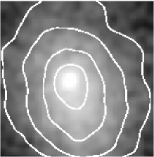
Figure 1: Chandra ACIS-S image (0.5-5 keV) of a $4.5\arcmin\times 4.5\arcmin$ region centered on A2589. The image has been smoothed with a gaussian filter with $\sigma=12\arcsec$. Smoothed contours overlaid are logarithmically spaced in intensity. Note the image has not been corrected for exposure variations, nor has the background been subtracted.

Table 1: Parameters from the Spectral Fits

	$R_{\rm in}$		$R_{\rm out}$		$T$	$Z_{\rm Fe}$	$norm$
Annulus	(arcmin)	(kpc)	(arcmin)	(kpc)	(keV)	(solar)	(10-3 cm-5)	$(\chi^{2}$/dof)
1	0	0	0.53	26	$3.16\pm 0.24$	$1.19\pm 0.35$	$1.22\pm 0.10$	$53.6/56$
2	0.53	26	0.82	40	$3.14\pm 0.24$	$0.65\pm 0.24$	$1.41\pm 0.10$	$68.7/57$
3	0.82	40	1.34	66	$3.30\pm 0.20$	$0.75\pm 0.21$	$2.72\pm 0.15$	$118.5/104$
4	1.34	66	1.85	91	$3.03\pm 0.19$	$0.64\pm 0.16$	$2.86\pm 0.14$	$128.2/107$
5	1.85	91	3.18	156	$3.18\pm 0.16$	$0.36\pm 0.09$	$6.74\pm 0.21$	$165.1/167$

Figure 2: ACIS-S3 spectra accumulated within (Left Panel) annulus #1 and (Right Panel) annulus #5. Each spectrum is fitted with an apec plasma model modified by Galactic absorption as discussed in §3.

In Figure 1 we display the ACIS-S3 image of A2589. The isophotes are regularly shaped and are approximately elliptical with $\epsilon=0.2-0.3$ over the region of interest. The centroid of the innermost contour is displaced with respect to that of the outer contours shown by $\approx 15\arcsec$. Very importantly, we see no evidence for disturbances or holes in the hot gas that are ubiquitous in the cores of cooling flow clusters as discussed in §1. In this paper we ignore the flattening of the X-ray isophotes and instead obtain circularly averaged spectral quantities (i.e., gas density and temperature) on the sky to construct the spherically averaged deprojected mass distribution.

We extracted spectra in concentric circular annuli located at the X-ray centroid computed within a radius of $20\arcsec$ with initial center on the peak of the X-ray emission. (We examine the sensitivity of our results to the chosen center position in §8.) The widths of the annuli were chosen to have approximately equal background-subtracted counts in the 0.5-5 keV band. Because of the high background we did not use the data for $R\gtrsim 3\arcmin$, and the widths of the annuli had to be relatively large. These restrictions resulted in a set of five annuli within $R=3.2\arcmin$ as listed in Table 1. We constructed ARF files for each annulus using the latest corrections that account for the time-dependent degradation in the quantum efficiency at lower energies. A single RMF file appropriate for the CTI-corrected S3 data was used.

For each annulus we fitted the background-subtracted spectrum with an apec thermal plasma modified by Galactic absorption ($4.15\times 10^{20}$ cm^-2). For the apec model we usually let the iron abundance be a free parameter, and the abundances of all the other elements are tied to iron in their solar ratios; i.e., we fit a metallicity. The spectral fitting was performed with xspec (Arnaud, 1996) using the $\chi^{2}$ method. Hence, we rebinned all spectral channels to have a minimum of 30 counts per energy bin. We take the solar abundances in xspec (v11.2.0bc) to be those given by Grevesse & Sauval (1998) which use the correct “new” photospheric value for iron which agrees also with the value obtained from solar-system meteorites (e.g., McWilliam, 1997). We restricted the spectral fitting between 0.5-5 keV to avoid calibration uncertainties at lower energies and systematic errors associated with the background subtraction at high energies. To estimate the statistical errors on the fitted parameters we simulated spectra for each annulus using the best-fitting models and fit the simulated spectra in exactly the same manner as done for the actual data. From 100 Monte Carlo simulations we compute the standard deviation for each free parameter which we quote as the “$1\sigma$” error. (We note that these $1\sigma$ error estimates generally agree very well with those obtained using the standard $\Delta\chi^{2}$ approach in xspec.)

The parameters obtained from the spectral fits are listed in Table 1. The simple one-temperature model is a good fit to the data in all annuli. In Figure 2 we show the ACIS-S3 spectra of the innermost and outermost annuli and the associated best-fitting one-temperature model. Visual inspection of Figure 2 reveals that the spectral shapes of annuli #1 and #5 are similar above $\sim 2$ keV indicating that they have similar temperatures. Near 1 keV the spectrum of annulus #1 is more peaked reflecting its larger iron abundance. In sum, the one-temperature model reveals a nearly isothermal gas but with evidence for a metallicity gradient similar to those observed in other clusters with a dominant central galaxy (e.g., Lewis et al., 2002; Ettori et al., 2002; Gastaldello & Molendi, 2002; Sanders & Fabian, 2002).

These results agree with those obtained using ROSAT PSPC data by David et al. (1996) within the relatively large statistical errors associated with the PSPC data. David et al. (1996) obtain a temperature of $T=1.7^{+1.0}_{-0.3}$ keV (90% conf.) within $R=1\arcmin$ which is marginally inconsistent with our results obtained with Chandra. However, spectral parameters obtained from X-ray spectra of groups and clusters can depend on a variety factors such as bandwidth (e.g., see Buote et al., 2003a, b). David et al. (1996) fitted models over 0.3-2 keV appropriate for the PSPC. If we use 0.5-2 keV we obtain $T\approx 2.5$ keV within $R=30\arcsec$ consistent with the PSPC result.

Although the fits are acceptable, we investigated whether they could be improved further. We allowed other elemental abundances to be free parameters. It was found that allowing silicon and oxygen to be free did offer significant (though not substantial) improvements in the fits in some annuli. Typically, both abundances fitted to low values (i.e., sub-solar ratios with respect to iron) but are consistent with the iron abundance within the estimated $1\sigma$ errors. Since it was also found that when allowing silicon and oxygen to be free the fitted temperatures and normalizations did not vary appreciably within their $1\sigma$ errors, we decided to keep silicon and oxygen tied to iron in the fits as done for the other elements.

We also found that adding another temperature component did not improve the fits much. For example, in the central annulus adding another temperature component improved $\chi^{2}$ by 3 but with the addition of two free parameters (one for temperature and one for normalization – abundances are tied to the first temperature component). The second temperature component ($T\approx 1$ keV) has only $\approx 1\%$ of the emission measure indicating that a single temperature component clearly dominates the ACIS-S spectra. If we add a high-temperature component ($T>10$ keV) to annulus #4 the fit is improved by $\Delta\chi^{2}=20$. This weak high-temperature component is almost certainly associated with incomplete background subtraction in this annulus. In §8 we discuss errors associated with the background and other systematic effects.

4 The Radial Profile of Gravitating Mass

4.1 Method

The approach we use to calculate the mass distribution follows closely our previous study of A2029 (Lewis et al., 2003). We approximate the hot gas in the cluster as spherically symmetric and in hydrostatic equilibrium so that the total gravitating mass is,

$$\hbox{{$M_{\rm grav}$}}(<r)=r{k_{B}T(r)\over G\mu m_{\rm p}}\left(-{d\ln\hbox{{$\rho_{\rm g}$}}\over d\ln r}-{d\ln T\over d\ln r}\right),$$ (1)

where $r$ is the radius in a three-dimensional volume, $\rho_{\rm g}$ is the gas mass density, $T$ is the gas temperature, $m_{p}$ is the atomic mass unit, $\mu$ is the mean atomic weight of the gas (taken to be 0.62), $k_{B}$ is Boltzmann’s constant, and $G$ is Newton’s constant. $M_{\rm grav}$ is the enclosed gravitating mass which is the sum of the masses of the stars, the gas, and the DM. We evaluate the derivatives of $\rho_{\rm g}$ and $T$ using parameterized models as discussed below. We note that spherical averaging of the data is appropriate for comparison to the spherically averaged DM profiles obtained from cosmological simulations which is a key goal of this paper.

We note that the cooling time of the gas is $\approx 1$ Gyr within the central annulus, indicating that some heat source is required to prevent the gas from cooling. Models of cluster cooling flows including both feedback from an AGN and thermal conduction appear to successfully prevent the gas from cooling (e.g., Brighenti & Mathews, 2003). In the context of this paradigm, since no substantial morphological disturbances in the X-ray image are currently observed in the core of A2589, this cluster presumably has had sufficient time to relax since the previous feedback episode.

4.2 Deprojected Radial Profiles of Gas Density and Temperature

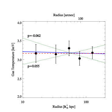
Figure 3: Left Panel: Chandra radial profile of the projected gas density squared ($\int\hbox{{$\rho_{\rm g}$}}^{2}dl$) obtained by dividing the $norm$ parameter of the apec model (Table 1) by the area of the annulus as described in §4.2. Horizontal bars indicate the sizes of the annuli used to extract spectra, and the sizes of the spherical shells used in our deprojected analysis. Overlaid is the best-fitting $\beta$-model (solid curve). Right Panel: Chandra radial temperature profile of A2589. Overlaid are the best-fitting isothermal (dashed (red) curve), and power-law (solid (blue) curve) models. Also shown are the $1\sigma$ limits for the power-law model (dotted (green) curves). The temperature data points refer to projected quantities (Table 1) while the temperature models are deprojected (Table 2).

Table 2: Deprojected Radial Profiles of Gas Density and Temperature

Gas Density
		$r_{c}$		$\hbox{{$\rho_{\rm g}$}}_{0}$
Model	$(\chi^{2}$/dof)	(kpc)	$\beta$	($10^{-26}$ g cm-3)
$\beta$	0.8/2	$40\pm 12$	$0.39\pm 0.04$	$1.93\pm 0.12$
Temperature
		$T_{100}$
Model	$(\chi^{2}$/dof)	(keV)	$p$
isothermal	1.0/4	$3.16\pm 0.22$	$0$
power law	1.0/3	$3.17\pm 0.43$	$-0.006\pm 0.06$

We first attempted to obtain three-dimensional gas parameters by performing a spectral deprojection procedure based on the “onion-peeling” method that we have used in previous studies (Buote, 2000; Buote et al., 2003a; Lewis et al., 2003). Because the S/N of the A2589 data is relatively low, we are unable to obtain precise constraints on the deprojected temperature and abundance profiles using this procedure (but see §8). Consequently, we projected parameterized models of the three-dimensional quantities, $\rho_{\rm g}$ and $T$, and fitted these projected models to the results obtained from our analysis of the data projected on the sky (Table 1). In this manner we obtained good constraints on the three-dimensional radial profiles of $\rho_{\rm g}$ and $T$. Note that for each annulus we assign a single radius value, $r\equiv[(r_{\rm out}^{3/2}+r_{\rm in}^{3/2})/2]^{2/3}$, where $r_{\rm in}$ and $r_{\rm out}$ are respectively the inner and outer radii of the annulus/shell. We found this prescription to provide an excellent estimate of the mean weighted radius in our previous study of A2029 (Lewis et al., 2003).

The $norm$ parameter of the apec model obtained from the spectral fits (see Table 1) is proportional to $\int\hbox{{$\rho_{\rm g}$}}^{2}dV$, where $dV$ represents the emitting volume. For our data in projection we have $dV=Adl$, where $A$ is the area of the annulus on the sky and $dl$ is the length element along the line of sight; i.e., $\int\hbox{{$\rho_{\rm g}$}}^{2}dl\propto norm/A$. (It is assumed that the plasma emissivity is constant along the line of sight which is a very good approximation for the nearly isothermal spectrum of A2589.) In Figure 3 we plot $\int\hbox{{$\rho_{\rm g}$}}^{2}dl$ along with the best-fitting $\beta$ model (Cavaliere & Fusco-Femiano, 1978),

$$\rho_{\rm g} = \hbox{{$\rho_{\rm g}$}}_{0}(1+r^{2}/r_{c}^{2})^{-3\beta/2}$$ (2)

$$\int\hbox{{$\rho_{\rm g}$}}^{2}dl = {\Gamma(\frac{1}{2})\Gamma(3\beta-\frac{1}{2})\over\Gamma(3\beta)}{\hbox{{$\rho_{\rm g}$}}_{0}^{2}r_{c}\over(1+R^{2}/r_{c}^{2})^{3\beta-0.5}},$$ (3)

where the integral is evaluated along the line of sight $(-\infty,+\infty)$, and $R$ is the radius of the annulus on the sky.. The best-fitting parameters, $1\sigma$ errors, and $\chi^{2}$ values are listed in Table 2. The errors are calculated by fitting the $norm$ profiles obtained for each Monte Carlo error simulation (§3). We find that the simple $\beta$ model is an excellent fit.

We modeled the temperature data as the emission-weighted projection of a power law profile,

$$T(r) = T_{100}\left(\frac{r}{100\,{\rm kpc}}\right)^{p}$$ (4)

$$\langle T(R)\rangle = \int\hbox{{$\rho_{\rm g}$}}^{2}\,T_{100}\left(\frac{\sqrt{R^{2}+l^{2}}}{100\,{\rm kpc}}\right)^{p}dl/\int\hbox{{$\rho_{\rm g}$}}^{2}dl,$$ (5)

where $T_{100}$ is the temperature at $r=100$ kpc, $\rho_{\rm g}$ is the $\beta$ model given above, and again $R$ is the radius of the annulus on the sky. The best-fitting model ($\langle T(R)\rangle$) is plotted in Figure 3 and the parameters and $1\sigma$ errors for $T(r)$ are given in Table 2. The temperature profile is nearly isothermal. This is illustrated by the excellent fit obtained for $p$ fixed to 0 (Figure 3 and Table 2).

4.3 Three-Dimensional Radial Mass Profile

Table 3: Parameters of Gravitating Matter and Dark Matter Radial Profiles

			$M_{100}$	$r_{s}$		$r_{\rm vir}$
Mass Model	$(\chi^{2}$/dof)	$\gamma$	$(10^{13}\hbox{{$M_{\sun}$}})$	(kpc)	$c$	(Mpc)
Gravitating Matter
power law	5.0/3	$1.63\pm 0.14$	$1.11\pm 0.44$	$\cdots$	$\cdots$	$\cdots$
NFW	2.0/3	$\cdots$	$\cdots$	$153\pm 362$	$6.6\pm 2.5$	$1.01\pm 0.32$
Dark Matter
power law	2.7/2	$1.65\pm 0.21$	$0.90\pm 0.33$	$\cdots$	$\cdots$	$\cdots$
NFW	1.9/2	$\cdots$	$\cdots$	$208\pm 865$	$4.9\pm 2.4$	$1.03\pm 0.51$

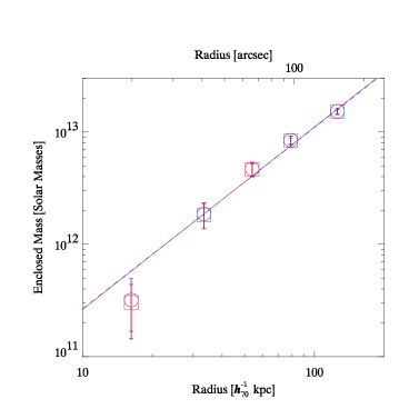
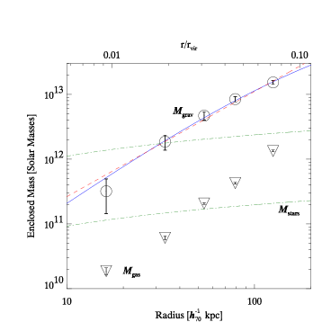
Figure 4: Left Panel: Total gravitating mass of the cluster for each radial bin obtained from the isothermal (open squares, red) and the power-law (open circles, blue) fits to the gas temperatures. The $\beta$-model parameterization for $\rho_{\rm g}$ was used in both cases. The mass points are fitted with corresponding power law functions (solid line, blue: power-law $T$ model, dashed line,red: isothermal $T$ model). Right Panel: Total gravitating mass (data points enclosed with open circles), overlaid with two different fitted models: NFW ((blue) solid curve) and power-law ((red) dashed line). Each model uses the power-law parameterization of the temperature profile. The enclosed gas mass is plotted as data points enclosed with open triangles. Also plotted is the mass range expected from the stars ((green) dot-dashed curves): The lower curve assumes $\hbox{{$M_{\rm stars}$}}/L_{V}=1\hbox{{$M_{\sun}$}}/\hbox{{$L_{\sun}$}}$ and the upper curve $\hbox{{$M_{\rm stars}$}}/L_{V}=12\hbox{{$M_{\sun}$}}/\hbox{{$L_{\sun}$}}$ (see §6). We have used large open symbols to identify the data points, as some of the error bars are difficult to see in this logarithmic plot. The upper axis shows the radius in units of the virial radius, ${\hbox{$r_{\rm vir}$}}=1.72$ Mpc.

Using the parameterized functions for the gas density and temperature just described, the radial mass distribution (eq. 1) becomes,

$$\hbox{{$M_{\rm grav}$}}(<r)=r{k_{B}T_{100}(r/100\,{\rm kpc})^{p}\over G\mu m_{\rm p}}\left({3\beta r^{2}/r_{c}^{2}\over 1+r^{2}/r_{c}^{2}}-p\right).$$ (6)

In Figure 4 we plot $M_{\rm grav}$ evaluated for each radial bin obtained from the isothermal (open squares, red) and the power-law (open circles, blue) fits to the gas temperatures. The mass profiles obtained from the isothermal and power-law models agree extremely well. Fitting a power law,

$$M(<r)=M_{100}\left(\frac{r}{100\,{\rm kpc}}\right)^{\gamma},$$ (7)

to the mass profile itself gives $\gamma=1.63\pm 0.14$ and $\gamma=1.61\pm 0.13$ for the power-law ($p$) and isothermal ($p=0$) temperature parameterizations respectively. The excellent agreement demonstrates that the mass profile is not particularly sensitive to the temperature parameterization, and thus we focus on the power-law temperature parameterization henceforth.

The NFW density and enclosed mass profile are given by,

$$\rho(r) = \frac{\rho_{c}(z)\delta_{c}}{(r/r_{s})(1+r/r_{s})^{2}},$$ (8)

$$M(<r) = 4\pi\rho_{c}(z)\delta_{c}r_{s}^{3}\left[\ln\left(\frac{r_{s}+r}{r_{s}}\right)-\frac{r}{r_{s}+r}\right],$$ (9)

where $\rho_{c}(z)=3H(z)^{2}/8\pi G$ is the critical density of the universe at redshift $z$, $r_{s}$ is the scale radius, and $\delta_{c}$ is a characteristic dimensionless density which, when expressed in terms of the concentration parameter $c$, takes the form,

$$\delta_{c}=\frac{200}{3}\frac{c^{3}}{\ln(1+c)-c/(1+c)}.$$ (10)

Hence, there are two free parameters for the NFW mass profile: $r_{s}$ and $c$. The virial radius, defined to be the radius where the enclosed average mass density equals $200\rho_{c}(z)$, is simply ${\hbox{$r_{\rm vir}$}}=cr_{s}$. We calculate $\rho_{c}(z)$ at the redshift of A2589 assuming $\hbox{{$\Omega_{\rm m}$}}=0.3$ and $\hbox{{$\Omega_{\Lambda}$}}=0.7$ today.

In Figure 4 we show the result of fitting an NFW model to the mass profile along with the power-law fit for comparison. The parameters for both models are listed in Table 3. The NFW model provides a very good fit to mass points, better than the power law model, though the power law is still a fair representation of the mass profile. Both models lie above the innermost data point. Excluding the innermost data point does not significantly change the results. For example, when omitting the inner mass point the power-law mass fit gives $\gamma=1.47\pm 0.15$ which is within $\approx 1\sigma$ of the value obtained when fitting all the points (Table 3). Similarly, we obtain a concentration parameter $c=7.8\pm 3.4$ for NFW when excluding the inner point which is quite consistent with the value given in Table 3. (We mention that a Hernquist model (Hernquist, 1990) fits as well as NFW ($\chi^{2}=1.9$ for 3 dof), but the Moore model is not quite as good a fit ($\chi^{2}=6.7$ for 3 dof).)

The virial radius ($r_{\rm vir}$) obtained from the NFW fit to $M_{\rm grav}$ is rather small ($1.01\pm 0.32$ Mpc) for a massive galaxy cluster, though our value does have a large uncertainty. It is consistent with the virial radius, ${\hbox{$r_{\rm vir}$}}=1.72\pm 0.32$ Mpc, obtained using the virial mass–temperature relation of Mathiesen & Evrard (2001) with the temperature of the isothermal model (Table 1).

5 Gas Mass, Gas Fraction, and $\Omega_{m}$

The radial profile of the enclosed mass of hot gas obtained from the $\beta$-model (eq. 2) is plotted in Figure 4. The gas fraction $(\hbox{{$f_{\rm gas}$}}=\hbox{{$M_{\rm gas}$}}/\hbox{{$M_{\rm grav}$}})$ is $0.059\pm 0.033$ in the inner radial bin and rises to $0.087\pm 0.006$ in the last radial bin; i.e., the gas mass is a minor contributor to the gravitating mass over the region studied. The gas fraction in the last radial bin may be safely considered to be a lower limit since simulations and other measurements at larger radii in clusters suggest $\hbox{{$f_{\rm gas}$}}=(0.2-0.3)h_{70}^{-3/2}$ (e.g., Allen et al., 2002). Assuming the global baryon fraction in A2589 is representative, then we place an upper limit on the present matter density, $\hbox{{$\Omega_{\rm m}$}}\leq\Omega_{\rm b}/\hbox{{$f_{\rm gas}$}}=0.56\pm 0.05$ where we have used $\Omega_{\rm b}h^{2}=0.024\pm 0.001$ for $h=0.7$ from recent measurements of the CMB (Spergel et al., 2003). We emphasize that our upper limit on $\Omega_{\rm m}$ results from underestimating the baryon fraction because (1) we do not measure a global value of $f_{\rm gas}$, and (2) we account for only the baryons associated with the hot gas.

6 Gravitating Mass-to-Stellar Light Ratio and the Stellar Mass Contribution

Figure 5: Ratio of gravitating mass to stellar light from the cD galaxy in A2589.

To calculate the ratio of gravitating mass to stellar light we used the fits to the $V$-band surface brightness profile of A2589 published by Malumuth & Kirshner (1985). These authors found that a King model with core radius $r_{c}=0.98h_{70}^{-1}$ kpc and a total luminosity of $2.3\times 10^{11}L_{V,\sun}h_{70}^{-2}$ provides a a good fit to surface brightness profile out to $R=130h_{70}^{-1}$ kpc. The King model fit translates to a volume light density profile, $\rho_{V}(r)=\rho_{V}(0)(1+r^{2}/r^{2}_{c})^{-3/2}$, where $\rho_{V}(0)=3.8L_{V,\sun}{\rm pc}^{-3}$. The enclosed luminosity as a function of radius in three dimensions $(L_{V}(<r))$ is calculated by integrating $\rho_{V}$ over the volume of the sphere of radius $r$. We plot $\hbox{{$M_{\rm grav}$}}(<r)/L_{V}(<r)$ in Figure 5.

$\hbox{{$M_{\rm grav}$}}/L_{V}$ climbs from $2.8\pm 1.5\,\hbox{{$M_{\sun}$}}/\hbox{{$L_{\sun}$}}$ at the inner radial bin to $73.6\pm 4.8\,\hbox{{$M_{\sun}$}}/\hbox{{$L_{\sun}$}}$ at the outer radial bin. At the resolution of our chosen radial bin sizes there is no evidence for a sharp transition in $\hbox{{$M_{\rm grav}$}}/L_{V}$ over the region studied.

Converting $L_{V}$ to stellar mass ($M_{\rm stars}$) is problematic because of the uncertain stellar mass-to-light ratio ($\hbox{{$M_{\rm stars}$}}/L_{V}$) of elliptical galaxies. Often stellar dynamical measurements of the cores of elliptical galaxies are taken as estimates for the stellar mass. But since such dynamical studies (like X-rays) are sensitive to the total gravitating mass, they cannot be relied upon to yield robust values of the stellar mass separated from the DM. Stellar population synthesis studies offer a direct method to calculate $\hbox{{$M_{\rm stars}$}}/L_{V}$ but unfortunately allow for a large range of values ($\hbox{{$M_{\rm stars}$}}/L_{V}=1-12\,\hbox{{$M_{\sun}$}}/\hbox{{$L_{\sun}$}}$) because of uncertainties associated with the stellar initial mass function, the age of the population(s), and the metallicity (e.g., Pickles, 1985; Maraston, 1999) – though see Mathews (1989) for arguments that the stellar mass is similar to the value determined from stellar dynamics.

In Figure 4 we plot $M_{\rm stars}$ for the cases $\hbox{{$M_{\rm stars}$}}/L_{V}=1\,\hbox{{$M_{\sun}$}}/\hbox{{$L_{\sun}$}}$ and $\hbox{{$M_{\rm stars}$}}/L_{V}=12\,\hbox{{$M_{\sun}$}}/\hbox{{$L_{\sun}$}}$ to show the allowed range from population synthesis studies of elliptical galaxies. The upper limit for $M_{\rm stars}$ essentially passes through the value of $M_{\rm grav}$ at the second radial bin ($r=33$ kpc) but greatly exceeds $M_{\rm grav}$ in the central radial bin. If $M_{\rm grav}$  in the central bin is reliable then $\hbox{{$M_{\rm stars}$}}/L_{V}$ must be small enough to match $\hbox{{$M_{\rm grav}$}}/L_{V}=2.8\pm 1.5\,\hbox{{$M_{\sun}$}}/\hbox{{$L_{\sun}$}}$ obtained from the X-ray analysis. Hence, we assume a plausible range of stellar mass-to-light ratios, $\hbox{{$M_{\rm stars}$}}/L_{V}=(1-7.4)\hbox{{$M_{\sun}$}}/\hbox{{$L_{\sun}$}}$, where the upper limit is the $3\sigma$ upper limit on $\hbox{{$M_{\rm grav}$}}/L_{V}$ in the central radial bin and the lower limit is determined by the population synthesis models.

7 The Dark Matter Radial Profile

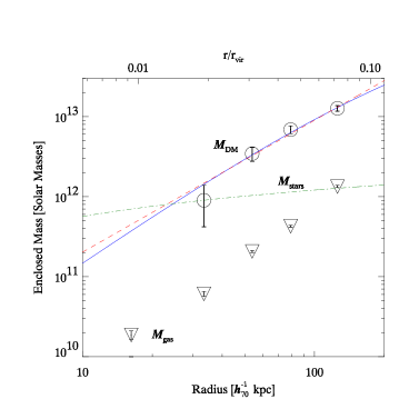
Figure 6: Same as Figure 4 except that $M_{\rm grav}$ is replaced by $M_{\rm DM}$, and $M_{\rm stars}$ is calculated for $\hbox{{$M_{\rm stars}$}}/L_{V}=6.1\,\hbox{{$M_{\sun}$}}/\hbox{{$L_{\sun}$}}$.

Inspection of Figure 4 reveals that the gravitating mass exceeds the combined masses of stars and hot gas for $r\gtrsim 0.02{\hbox{$r_{\rm vir}$}}$ indicating that DM dominates over most of the region studied. We write the mass in DM as, $\hbox{{$M_{\rm DM}$}}=\hbox{{$M_{\rm grav}$}}-\hbox{{$M_{\rm gas}$}}-\hbox{{$M_{\rm stars}$}}$, where $M_{\rm gas}$ and $M_{\rm stars}$ are described in §5 and §6. For $M_{\rm stars}$ we define a fiducial value by requiring that interior to the effective radius ($R_{e}=32.6$ kpc, Malumuth & Kirshner 1985) we have $\hbox{{$M_{\rm DM}$}}=\hbox{{$M_{\rm stars}$}}$. This definition allows for a fairly smooth transition between stellar-dominated and DM-dominated regimes and yields $\hbox{{$M_{\rm stars}$}}/L_{V}=6.1\,\hbox{{$M_{\sun}$}}/\hbox{{$L_{\sun}$}}$ consistent with the values determined in §6.

In Figure 6 we plot $M_{\rm stars}$ and $M_{\rm DM}$ corresponding to this fiducial stellar model. The inner data point cannot be seen in the figure because the dark mass is negative there, $\hbox{{$M_{\rm DM}$}}=-4.0\pm 1.7\times 10^{11}\hbox{{$M_{\sun}$}}$, though it has large error. Consequently, we exclude the inner radial bin from fits to $M_{\rm DM}$ when using the fiducial value of $\hbox{{$M_{\rm stars}$}}/L_{V}$.

We plot the best-fitting power-law and NFW models to $M_{\rm DM}$ in Figure 6; the fit parameters are listed in Table 3. The quality of the fits and the parameter values of the DM models are consistent with those obtained for the gravitating mass within the $1\sigma$ errors. (Note: including the inner (negative) data point results in fits that are of significantly lower quality: $\chi^{2}=19.4$ for power law and $\chi^{2}=18.5$ for NFW, each with 3 dof.) Similar to the fits to $M_{\rm grav}$, the Moore model does not fit quite as well as NFW ($\chi^{2}=3.6$ for 2 dof), but the Hernquist model provides a comparable fit ($\chi^{2}=1.8$ for 2 dof). The core parameter for the Hernquist model is poorly constrained ($a=0.34\pm 0.77$ Mpc).

8 Systematic Error Budget for $M_{\rm DM}$

Table 4: Error Budget for Dark Matter Fits

	Best	$\Delta$Statistical	$\Delta$Background	$\Delta$$M_{\rm stars}$	$\Delta$Deproj
Power Law:
$\gamma$	$1.65$	$\pm 0.21$	$(+0.17,-0.16)$	$(+0.06,-0.00)$	$+0.35$
NFW:
$c$	4.9	$\pm 2.4$	$(+1.9,-1.7)$	$(+1.2,-0.6)$	$-3.8$
$r_{\rm vir}$(Mpc)	1.0	$\pm 0.5$	$(+0.3,-0.2)$	$(+0.06,-0.05)$	$+1.9$

This section provides an assessment of the magnitude of systematic errors on the fits to $M_{\rm DM}$.

X-ray Background: To examine the sensitivity of the measured dark matter properties to reasonable background errors we repeated our entire analysis using the standard background templates and correction files (§2) renormalized to have count rates $\pm 20\%$ of their nominal values. We find that the derived gas density profile is hardly affected while the temperature profile is modified within the $1\sigma-1.5\sigma$ errors: $p=(-0.09,0.07)$ for these different background levels. The effect on the DM fits is less than the $1\sigma$ errors in the DM model parameters as shown in Table 4. We also examined whether the DM fits were systematically different if the normalization of the background was allowed to be a free parameter during the fits. We found that the DM fits are fully consistent with the results quoted above. We note, however, that in this case the best-fitting temperatures ($\approx 20\%$) and abundances ($\approx 40\%$) are lower than the values listed in Table 1, although the differences are significant only at the $\approx 2\sigma$ level.

Stellar Mass: In Table 4 we quote the ranges in model parameters fitted to $M_{\rm DM}$ considering the variation in $M_{\rm stars}$ implied by $\hbox{{$M_{\rm stars}$}}/L_{V}=(1-7.4)\,\hbox{{$M_{\sun}$}}/\hbox{{$L_{\sun}$}}$ (see §6). Note that for $\hbox{{$M_{\rm stars}$}}/L_{V}=1\hbox{{$M_{\sun}$}}/\hbox{{$L_{\sun}$}}$ the inner radial bin for $M_{\rm DM}$ is positive, and so we included it in the fits in Table 4. Uncertainties associated with the stellar mass are within the $1\sigma$ errors.

Center: Since the X-ray centroid varies with radius we examined the sensitivity of our results to the centroid. For comparison to our results obtained using the centroid computed within a circular aperture of radius $20\arcsec$, we used a radius of $3\arcmin$. Using this larger radius we obtain a centroid offset by $\approx 8\arcsec$ from the previous value. However, we find that the results obtained for the DM fits change negligibly ($<1\%$) when using the different centroid.

Deprojection Method: Our method to deproject the gas density and temperature uses the projections of parameterized models (§4.2). For comparison, we also performed a non-parametric deprojection using the “onion-peeling” method as implemented in our previous studies (e.g., Buote, 2000; Buote et al., 2003a; Lewis et al., 2003). To obtain stable deprojected parameters for the A2589 Chandra data we imposed the following restrictions: (1) the deprojected temperatures in annuli #3-5 were confined to the $1\sigma$ limits in Table 1, and (2) the deprojected metallicities were set to those in Table 1. Because of these restrictions the results obtained from this deprojection should only be viewed as an indicator of the sensitivity of the results to deprojection and not as the preferred values. We found that the deprojected temperature and density profiles give results consistent with those obtained from the parametric deprojection when fitted with the same models in three dimensions. However, the gas density is more centrally peaked than indicated by the $\beta$ model and thus, like in A2029 (Lewis et al., 2003), we find that adding a central cusp to the $\beta$ model provides a better fit. We find that $M_{\rm DM}$ is small, but positive, in the central bin. Using all five data points we obtain the results reflected in Table 4 for fits to the DM.

9 Conclusions

Our analysis of the Chandra data indicates that from the largest radius probed ($r=0.07{\hbox{$r_{\rm vir}$}}$) down to $r\approx 0.02{\hbox{$r_{\rm vir}$}}$ the dominant contributor to the gravitating matter in A2589 is the DM. Over this region the radial profile of the DM is fitted well by the NFW and Hernquist profiles predicted by CDM. (These models fit the gravitating matter well down to $r=0.009{\hbox{$r_{\rm vir}$}}$.) The inferred value of $r_{\rm vir}$ of the NFW model is consistent (within the relatively large measurement errors) with that expected from CDM simulations (1.7 Mpc, see §4.3); equivalently, the concentration parameter $c=4.9\pm 2.4$ is in the range expected for a massive cluster (Navarro et al., 1997). The DM profile over this region is also described well by a power law, $M(<r)\propto r^{\gamma}\rightarrow\rho\propto r^{-\alpha}$ where $\alpha=3-\gamma$. We find $\alpha=1.35\pm 0.21$ (statistical error, see §8) which is consistent with the NFW value $\alpha=1$ (and Moore value of $\alpha=1.5$) but is significantly larger than $\alpha\approx 0.5$ found in LSB galaxies (e.g., Swaters et al., 2000) and expected from SIDM models (Spergel & Steinhardt, 2000). We note that the profile of the gravitating matter ($\alpha=1.37\pm 0.14$) is also very consistent with the DM profile and with CDM predictions (El-Zant et al., 2003).

The DM properties of A2589 agree very well with those obtained for A2029 (Lewis et al., 2003). Because the cores of these clusters are undisturbed by interactions from a central radio source, the results we have obtained for their core DM distributions provide critical confirmation of (in some respects) similar results obtained from other otherwise-relaxed clusters with disturbed cores (most notably Hydra-A, David et al. 2001) and clarify ambiguous cases like A1795 (Ettori et al., 2002). Furthermore, the evidence that the NFW-CDM profile is a good fit to cluster DM halos on larger scales $(0.1{\hbox{$r_{\rm vir}$}}\lesssim r<0.5{\hbox{$r_{\rm vir}$}})$ (e.g., Allen et al., 2002; Pratt & Arnaud, 2002) is extended down to $r\sim 0.01{\hbox{$r_{\rm vir}$}}$ by our complementary analyses of the Chandra data of A2029 and A2589. This agreement of cluster DM profiles with the NFW model is also supported by the recent weak-lensing analysis of several clusters by Dahle et al. (2003) and the joint lensing-X-ray study of Arabadjis et al. (2002).

In sum, the current evidence from X-ray and lensing studies indicates that the radial DM profiles for cluster-sized DM halos are consistent with CDM predictions within the expected cosmological scatter (Bullock et al., 2001). The disagreement between the NFW-CDM profile and the flatter profiles observed for LSB galaxies indicates that either CDM simulations are adequate for clusters but inadequate for LSB galaxies or the interpretations of the measurements of the DM profiles for LSB galaxies are in error. Some recent studies have indeed suggested that systematic errors could account for the flat density profiles obtained for LSB galaxies (e.g., Swaters et al., 2003).

Future X-ray and lensing studies of the DM in other (relaxed) cluster cores are essential to refine the constraints on the DM properties obtained from these initial studies and to quantify precisely the cosmological scatter.

References

- Allen et al. (2002) Allen, S. W., Schmidt, R. W., & Fabian, A. C. 2002, MNRAS, 334, L11
- Arabadjis et al. (2002) Arabadjis, J. S., Bautz, M. W., & Garmire, G. P. 2002, ApJ, 572, 66
- Arnaud (1996) Arnaud, K. A. 1996, in ASP Conf. Ser. 101: Astronomical Data Analysis Software and Systems V, Vol. 5, 17
- Bauer et al. (2000) Bauer, F. E., Condon, J. J., Thuan, T. X., & Broderick, J. J. 2000, ApJS, 129, 547
- Brighenti & Mathews (2003) Brighenti, F. & Mathews, W. G. 2003, ApJ, 587, 580
- Bullock et al. (2001) Bullock, J. S., Kolatt, T. S., Sigad, Y., Somerville, R. S., Kravtsov, A. V., Klypin, A. A., Primack, J. R., & Dekel, A. 2001, MNRAS, 321, 559
- Buote (2000) Buote, D. A. 2000, ApJ, 539, 172
- Buote et al. (2003a) Buote, D. A., Lewis, A. D., Brighenti, F., & Mathews, W. G. 2003a, ApJ, 594, 741
- Buote et al. (2003b) —. 2003b, ApJ, 595, 151
- Buote & Tsai (1996) Buote, D. A. & Tsai, J. C. 1996, ApJ, 458, 27
- Cavaliere & Fusco-Femiano (1978) Cavaliere, A. & Fusco-Femiano, R. 1978, A&A, 70, 677
- Dahle et al. (2003) Dahle, H., Hannestad, S., & Sommer-Larsen, J. 2003, ApJ, 588, L73
- Davé et al. (2001) Davé, R., Spergel, D. N., Steinhardt, P. J., & Wandelt, B. D. 2001, ApJ, 547, 574
- David et al. (1996) David, L. P., Jones, C., & Forman, W. 1996, ApJ, 473, 692
- David et al. (2001) David, L. P., Nulsen, P. E. J., McNamara, B. R., Forman, W., Jones, C., Ponman, T., Robertson, B., & Wise, M. 2001, ApJ, 557, 546
- Dubinski (1998) Dubinski, J. 1998, ApJ, 502, 141
- El-Zant et al. (2003) El-Zant, A., Hoffman, Y., Primack, J., Combes, F., & Shlosman, I. 2003, apJ Letters, submitted (astro-ph/0309412)
- Ettori et al. (2002) Ettori, S., Fabian, A. C., Allen, S. W., & Johnstone, R. M. 2002, MNRAS, 331, 635
- Evrard et al. (1996) Evrard, A. E., Metzler, C. A., & Navarro, J. F. 1996, ApJ, 469, 494
- Fabian et al. (2000) Fabian, A. C., Sanders, J. S., Ettori, S., Taylor, G. B., Allen, S. W., Crawford, C. S., Iwasawa, K., Johnstone, R. M., & Ogle, P. M. 2000, MNRAS, 318, L65
- Gastaldello & Molendi (2002) Gastaldello, F. & Molendi, S. 2002, ApJ, 572, 160
- Grevesse & Sauval (1998) Grevesse, N. & Sauval, A. J. 1998, Space Science Reviews, 85, 161
- Hernquist (1990) Hernquist, L. 1990, ApJ, 356, 359
- Jones & Forman (1999) Jones, C. & Forman, W. 1999, ApJ, 511, 65
- Lewis et al. (2003) Lewis, A. D., Buote, D. A., & Stocke, J. T. 2003, ApJ, 586, 135
- Lewis et al. (2002) Lewis, A. D., Stocke, J. T., & Buote, D. A. 2002, ApJ, 573, L13
- Malumuth & Kirshner (1985) Malumuth, E. M. & Kirshner, R. P. 1985, ApJ, 291, 8
- Maraston (1999) Maraston, C. 1999, in ASP Conf. Ser. 163: Star Formation in Early Type Galaxies, 28
- Markevitch et al. (2003) Markevitch, M., Bautz, M. W., Biller, B., Butt, Y., Edgar, R., Gaetz, T., Garmire, G., Grant, C. E., Green, P., Juda, M., Plucinsky, P. P., Schwartz, D., Smith, R., Vikhlinin, A., Virani, S., Wargelin, B. J., & Wolk, S. 2003, ApJ, 583, 70
- Mathews (1989) Mathews, W. G. 1989, AJ, 97, 42
- Mathiesen et al. (1999) Mathiesen, B., Evrard, A. E., & Mohr, J. J. 1999, ApJ, 520, L21
- Mathiesen & Evrard (2001) Mathiesen, B. F. & Evrard, A. E. 2001, ApJ, 546, 100
- McWilliam (1997) McWilliam, A. 1997, ARA&A, 35, 503
- Mohr et al. (1995) Mohr, J. J., Evrard, A. E., Fabricant, D. G., & Geller, M. J. 1995, ApJ, 447, 8
- Moore et al. (1999) Moore, B., Quinn, T., Governato, F., Stadel, J., & Lake, G. 1999, MNRAS, 310, 1147
- Navarro et al. (1997) Navarro, J. F., Frenk, C. S., & White, S. D. M. 1997, ApJ, 490, 493
- Perlmutter et al. (1999) Perlmutter, S., Aldering, G., Goldhaber, G., Knop, R. A., Nugent, P., Castro, P. G., Deustua, S., Fabbro, S., Goobar, A., Groom, D. E., Hook, I. M., Kim, A. G., Kim, M. Y., Lee, J. C., Nunes, N. J., Pain, R., Pennypacker, C. R., Quimby, R., Lidman, C., Ellis, R. S., Irwin, M., McMahon, R. G., Ruiz-Lapuente, P., Walton, N., Schaefer, B., Boyle, B. J., Filippenko, A. V., Matheson, T., Fruchter, A. S., Panagia, N., Newberg, H. J. M., Couch, W. J., & The Supernova Cosmology Project. 1999, ApJ, 517, 565
- Pickles (1985) Pickles, A. J. 1985, ApJ, 296, 340
- Pratt & Arnaud (2002) Pratt, G. W. & Arnaud, M. 2002, A&A, 394, 375
- Sanders & Fabian (2002) Sanders, J. S. & Fabian, A. C. 2002, MNRAS, 331, 273
- Spergel & Steinhardt (2000) Spergel, D. N. & Steinhardt, P. J. 2000, Physical Review Letters, 84, 3760
- Spergel et al. (2003) Spergel, D. N., Verde, L., Peiris, H. V., Komatsu, E., Nolta, M. R., Bennett, C. L., Halpern, M., Hinshaw, G., Jarosik, N., Kogut, A., Limon, M., Meyer, S. S., Page, L., Tucker, G. S., Weiland, J. L., Wollack, E., & Wright, E. L. 2003, apJ, submitted (astro-ph/0302209)
- Swaters et al. (2000) Swaters, R. A., Madore, B. F., & Trewhella, M. 2000, ApJ, 531, L107
- Swaters et al. (2003) Swaters, R. A., Verheijen, M. A. W., Bershady, M. A., & Andersen, D. R. 2003, ApJ, 587, L19
- Townsley et al. (2002) Townsley, L. K., Broos, P. S., Nousek, J. A., & Garmire, G. P. 2002, nuclear Instruments and Methods in Physics Research, in press (astro-ph/0111031)
- Tsai et al. (1994) Tsai, J. C., Katz, N., & Bertschinger, E. 1994, ApJ, 423, 553