A simple but efficient algorithm
for multiple-image deblurring

We consider the simultaneous deblurring of a set of noisy images whose point spread functions are different but known and spatially invariant, and the noise is Gaussian. Currently available iterative algorithms that are typically used for this type of problem are computationally expensive, which makes their application for very large images impractical. We present a simple extension of a classical least-squares (LS) method where the multi-image deblurring is efficiently reduced to a computationally efficient single-image deblurring. In particular, we show that it is possible to remarkably improve the ill-conditioning of the LS problem by means of stable operations on the corresponding normal equations, which in turn speed up the convergence rate of the iterative algorithms. The performance and limitations of the method are analyzed through numerical simulations. Its connection with a column weighted least-squares approach is also considered in an appendix.

1 Introduction

An important problem in image processing is the simultaneous deblurring of a set of observed images (of a fixed object), where each image is degraded by a different spatially invariant point spread function (PSF). For example, data obtained by the Large Binocular Telescope (LBT). This instrument consists of two $8.4{\rm m}$ mirrors on a common mount with a spacing of $14.4{\rm m}$ between the centers (Angel et al. 1998). For a given orientation of the telescope, the diffraction-limited resolution along the center-to-center baseline is equivalent to that of a $22.8{\rm m}$ mirror, while the resolution along the perpendicular direction is that of a single $8{\rm m}$ mirror. A possible way to obtain an image with an improved and uniform spatial resolution is to simultaneously deconvolve the images taken with different orientations of the telescope. Another example is the multi-frequency observations of the Cosmic Microwave Background (CMB) obtained from satellites such as PLANCK. In fact, although some other physical components are present at the microwave frequencies, the images taken at high galactic latitudes are expected to be almost entirely dominated by the CMB contribution in a large range of observing frequencies (e.g., see Stolyarov et al. 2002). Since the PSFs corresponding to the images obtained at the various frequencies can be quite dissimilar, simultaneous deblurring can be useful for improving the extraction of CMB information from the data.

Although a vast literature on the classical problem of single-image deblurring is available, much less has been published on multiple-image deblurring. An excellent general review is Bertero & Boccacci (2000b). In addition, Tegmark (1999) provides some material more directly related to CMB studies. But one of the more serious limitations of the methods currently available is that, although able to provide satisfactory results, they are quite expensive in terms of computational requirements. Thus, these methods may be quite difficult to use for the very large images ($\approx 10^{6}-10^{8}$ pixels) expected from LBT and PLANCK observations. It is clear that more efficient methods must be developed; the aim of this paper is to provide one such approach.

In Sect. 2 we formalize the problem and propose an efficient solution in Sect. 3. Some of its possible limitations are considered in Sect. 4. In Sect. 5 we study its performance through numerical experiments, and also compare it to that of other methods currently available in the literature. Finally, Sect. 7 closes with some final comments and conclusions.

2 Formalization of the problem

Suppose one has $p$ observed images, $g_{j}(x,y)$, $j=1,2,\ldots,p$, of a fixed two-dimensional object $f_{0}(x,y)$, each of which is degraded by a different spatially invariant blurring operator. That is,

$$g_{j}(x,y)=\iint K_{j}(x-x^{\prime},y-y^{\prime})f_{0}(x^{\prime},y^{\prime})dx^{\prime}dy^{\prime},$$ (1)

where, for each $j$, $K_{j}(x,y)$ is a space invariant PSF.

The image restoration problem of interest is to find an estimate $f(x,y)$ of $f_{0}(x,y)$ given the observed images $\{g_{j}(x,y)\}$ and the known PSFs $\{K_{j}(x,y)\}$.

In practice, the experimental images are discrete $N\times N$ arrays of pixels (for simplicity, we assume square images) contaminated by noise. Therefore model (1) has to be recast in the form

$$g_{j}(m,n)=\sum_{m^{\prime},n^{\prime}=0}^{N-1}K_{j}(m-m^{\prime},n-n^{\prime})f_{0}(m^{\prime},n^{\prime})+w_{j}(m,n),$$ (2)

where $w_{j}(m,n)$ is additive Gaussian white noise. For the moment, we assume constant standard deviations across images: $\sigma_{w_{j}}=\sigma_{w}$.

If the central peak (i.e., support) of each PSF is much smaller than the image, and if the object does not have structures near the image boundaries, then the convolution product in Eq. (2) can be well approximated by cyclic convolution. As is well known, such an approximation is quite useful since it permits rewriting Eq. (2) as

$$\hat{g}_{j}(m,n)=\hat{K}_{j}(m,n)\hat{f}_{0}(m,n)+\hat{w}_{j}(m,n),$$ (3)

where the symbol “$\leavevmode\nobreak\ \hat{}\leavevmode\nobreak\$” denotes the Discrete Fourier Transform (DFT).

One approach to compute an estimate of $f_{0}$ is to pose the image restoration problem as a least-squares (LS) problem, which is equivalent to a maximum likelihood approach in the case of white Gaussian noise. In order to outline the LS approach, it is helpful to use matrix-vector notation: Eq. (2) can be rewritten as

$$\boldsymbol{g}_{j}=\boldsymbol{A}_{j}\boldsymbol{f}_{0}+\boldsymbol{w}_{j},$$ (4)

where the arrays $\boldsymbol{g}$, $\boldsymbol{f}_{0}$ and $\boldsymbol{w}_{j}$ are obtained by column stacking $g_{j}(m,n)$, $f_{0}(m,n)$, and $w_{j}(m,n)$, respectively. $\boldsymbol{A}_{j}$ is the block-circulant matrix defined by cyclic convolution with the $j$th PSF. The LS estimate $\boldsymbol{f}$ can then be expressed in the form:

$$\boldsymbol{f}=\arg\min\,\sum_{j=1}^{p}\|\boldsymbol{A}_{j}\boldsymbol{f}-\boldsymbol{g}_{j}\|^{2}.$$ (5)

It is not difficult to see that $\boldsymbol{f}$ is the solution of the normal equations

$$\sum_{j=1}^{p}\boldsymbol{A}_{j}^{T}\boldsymbol{A}_{j}\boldsymbol{f}=\sum_{j=1}^{p}\boldsymbol{A}_{j}^{T}\boldsymbol{g}_{j},$$ (6)

where $\boldsymbol{A}_{j}^{T}$ denotes the transpose of the block-circulant matrix $\boldsymbol{A}_{j}$. The DFT of both sides of Eq. (6) provides

$$\hat{f}(m,n)\sum_{j=1}^{p}|\hat{K}_{j}(m,n)|^{2}=\sum_{j=1}^{p}\hat{K}_{j}^{*}(m,n)\hat{g}_{j}(m,n)=\hat{\vartheta}(m,n),$$ (7)

with symbol “$\leavevmode\nobreak\ {}^{*}\leavevmode\nobreak\$” denoting complex conjugation. This equation shows that the multi-image LS deblurring problem (5) is equivalent to classical one-image LS deblurring where the “observed” image is $\hat{g}(m,n)=\hat{\vartheta}(m,n)$ and the PSF is $\hat{K}(m,n)=\sum_{j=1}^{p}|\hat{K}_{j}(m,n)|^{2}$. As is well known, the direct LS estimate given by the inverse DFT of

$$\hat{f}(m,n)=\frac{\sum_{j}\hat{K}_{j}^{*}(m,n)\hat{g}_{j}(m,n)}{\sum_{j}|\hat{K}_{j}(m,n)|^{2}}$$ (8)

can be very unstable. For white noise, the mean square error (MSE) of (8) is

$${\rm E}[\|\boldsymbol{f}-\boldsymbol{f}_{0}\|^{2}]=\sigma^{2}_{w}\sum_{m,n}\frac{1}{\sum_{j}|\hat{K}_{j}(m,n)|^{2}}.$$ (9)

The quantities $\hat{K}_{j}(m,n)$ can be very close to zero at high frequencies because the PSFs are almost band-limited in practice. Consequently, the MSE can be very large, which indicates that the LS estimate is unstable. The main task of any deblurring method consists of stabilizing the solution by somehow limiting the values of such terms. Various methods have been proposed in the literature (e.g., see the review by Bertero & Boccacci 2000b). For example, the Tikhonov estimate $\boldsymbol{f}^{(\mu)}$ is defined as

$$\boldsymbol{f}^{(\mu)}=\arg\min\,\left[\,\sum_{j=1}^{p}\|\boldsymbol{A}_{j}\boldsymbol{f}-\boldsymbol{g}_{j}\|^{2}+\mu\|\boldsymbol{f}\|^{2}\,\right],$$ (10)

where $\mu$ is a positive scalar called the regularization parameter. The additional penalty term (weighted by $\mu$) has the effect of limiting the energy of $\boldsymbol{f}$. In fact, it is possible to see that

$$\hat{f}^{(\mu)}(m,n)=\frac{\sum_{j}\hat{K}_{j}^{*}(m,n)\hat{g}_{j}(m,n)}{\mu+\sum_{j}|\hat{K}_{j}(m,n)|^{2}},$$ (11)

where it is evident that the parameter $\mu$ smooths out the influence of the smallest values of $\hat{K}_{j}(m,n)$. If both the numerator and the second term in the denominator are computed and stored, then for each value of $\mu$ the computation of $\boldsymbol{f}^{(\mu)}$ requires $N^{2}$ divisions + $N^{2}$ sums + one two-dimensional DFT. This means that the Tikhonov method is computationally efficient, but it is not always flexible enough to allow the implementation of constraints such as positivity of the solution.

Iterative methods provide an alternative methodology that exploits the semiconvergence property of iterative inversion algorithms and can be easily implemented with many different types of constraints on the solution. Two examples (which provide constrained positive solutions) are the Projected Landweber (PL) method and the Iterative Space Reconstruction Algorithm (ISRA) (see Bertero & Boccacci 2000b). But, although flexible, these methods are expensive from the computational point of view, especially in situations of slow convergence (for each iteration, a couple of two-dimensional DFTs is required).

3 A more efficient approach

The main limitation of the methods mentioned in the previous section is that they are based on the normal equations (7). The resulting deblurring problem is much more ill-conditioned (i.e., the PSF is much broader) than implied by each of the models (2) because the coefficients $\hat{K}(m,n)$ in Eq. (7) are squared. The most important consequence is that the convergence of the iterative algorithms can be remarkably slowed with obvious consequence on the computational cost. However, by multiplying both sides of Eq. (7) by a function $\hat{K}_{j_{0}}(m,n)$, we can rewrite Eq. (7) in the form

$$\hat{K}_{j_{0}}(m,n)\hat{f}(m,n)$$ (12)

$$=\frac{\hat{g}_{j_{0}}(m,n)+\sum_{j\neq j_{0}}[\hat{K}_{j}^{*}(m,n)/\hat{K}_{j_{0}}^{*}(m,n)]\hat{g}_{j}(m,n)}{1+\sum_{j\neq j_{0}}[|\hat{K}_{j}(m,n)|^{2}/|\hat{K}_{j_{0}}(m,n)|^{2}]}$$

$$=\hat{\zeta}(m,n),$$

where

$$\hat{K}_{j_{0}}(m,n)=\max[\hat{K}_{1}(m,n),\hat{K}_{2}(m,n),\ldots,\hat{K}_{p}(m,n)].$$ (13)

Here the operator $\max[\leavevmode\nobreak\ ]$ extracts the element in the array with the largest modulus, and $j_{0}$ is the value of the corresponding index $j$. In the case that two or more PSFs whose DFTs, for a given frequency $(m,n)$, have the same modulus, it is sufficient to choose one of the $\hat{K}_{j}(m,n)$ according to a rule that preserves the symmetry of the DFT of a real PSF. As already noted for model (7), model (12) is also equivalent to a classical LS deblurring, but now the “observed” image is $\hat{\zeta}(m,n)$ and the PSF is $\hat{K}_{j_{0}}(m,n)$.

By construction, $\hat{K}_{j_{0}}(m,n)$ is the PSF whose energy distribution is maximally spread in the Fourier domain and therefore it corresponds to a PSF whose energy distribution is maximally concentrated in the spatial domain.

Figure 1: Comparison between the PSF corresponding to Eq. (7) (left panel) with that corresponding to Eq. (12) (right panel) for the numerical experiments presented in Sect. 5.

Figure 2: Slice comparison of the two-dimensional classical Hanning and rectangular windows with the modified Hanning window ($N_{w}=20$).

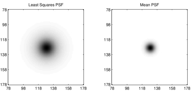
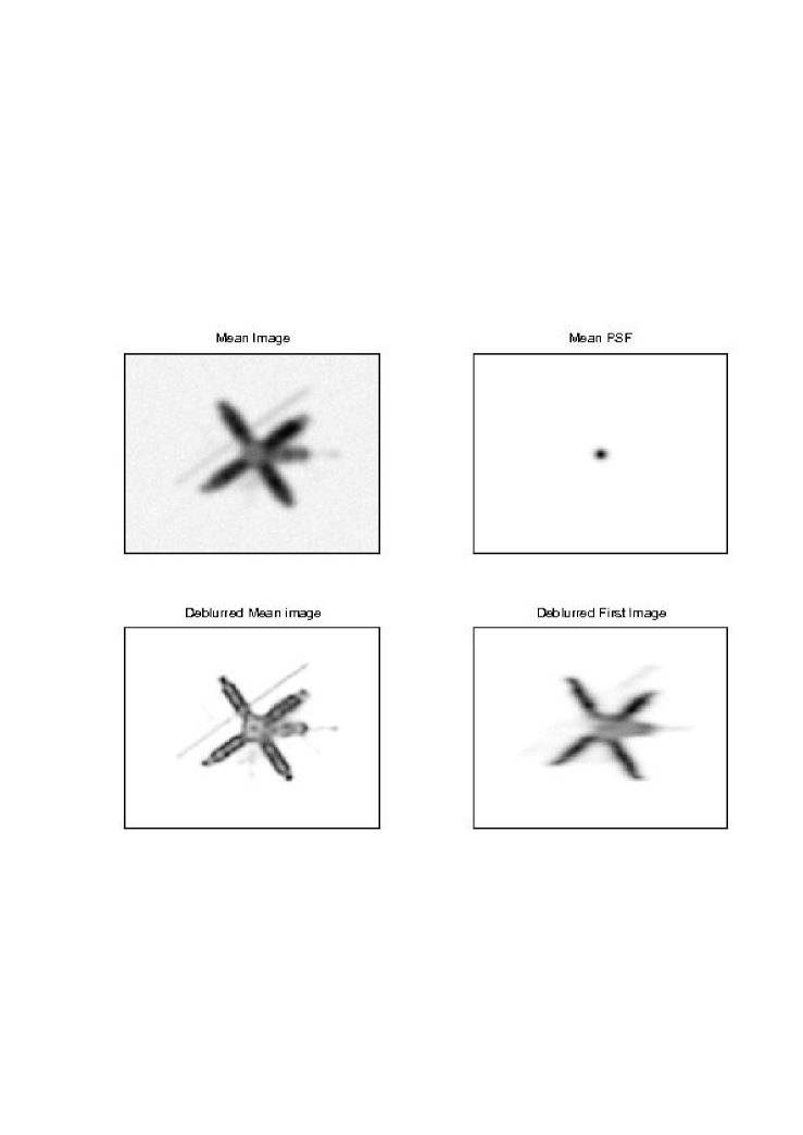
This means that $\hat{\zeta}(m,n)$ can be considered a sort of deblurred version of $\hat{\vartheta}(m,n)$ (see Fig. 1). In other words, the conditioning of system (12) is much better than that of system (7) (this is because $\hat{K}_{j_{0}}(m,n)$ is not obtained by squaring the coefficients $\hat{K}_{j}(m,n)$). The important point is that this result has been obtained through stable operations. From these considerations, improvements in the computational costs are to be expected. In addition, by formulating the problem in terms of single-image deblurring, there is a gain in flexibility as standard deblurring algorithms can be used.

In Appendix A, it is shown that $\hat{\zeta}(m,n)$ is equivalently obtained by transforming the LS problem (5) into a column weighted LS problem.

4 Two potential problems

Although simple and potentially very effective, the procedure presented in the previous sections has two potential drawbacks.

The first concerns the statistical properties of the noise component of $\zeta(m,n)$. In particular, even if the original noise $\boldsymbol{w}_{j}$ is white (i.e., a process with flat spectrum), the noise component of $\zeta(m,n)$ has a power-spectrum proportional to $|\hat{K}_{j_{0}}(m,n)|^{2}/\sum_{j}|\hat{K}_{j}(m,n)|^{2}$. This is a direct consequence of having used the normal equations (7) to solve the LS problem (5) and may have deleterious effects on automatic methods for stopping the iterations or estimating the regularization parameters since they assume that noise is white. For example, in our simulations the generalized cross validation (GCV) method (which may be used to estimate the optimal value of $\mu$ in the Tikhonov approach, see Vogel 2002) consistently produced values that were too small.

Figure 3: Original image, blurred version and blurred + noise version of the first image of the set (see text) and corresponding PSF. The images are $256\times 256$ pixels.

Figure 4: Mean image $\zeta(m,n)$ and corresponding PSF for the image shown in Fig. 3, deblurred version of $\zeta(m,n)$, and deblurred version of the first image of the set (see text). The deblurring was done with CGLS. The images shown are the ones with the smallest standard deviation of the true residuals; for the mean image and first image of the set these are, respectively, $6.57\times 10^{-2}$ and $8.67\times 10^{-2}$.

Figure 5: Mean image $\zeta(m,n)$ and corresponding PSF for the image shown in Fig. 3, deblurred version of $\zeta(m,n)$, and deblurred version of the first image of the set (see text). The deblurring was done with MRNSD. The images shown are the ones with the smallest standard deviation of the true residuals; for the mean image and the first image of the set these are $5.92\times 10^{-2}$ and $8.49\times 10^{-2}$, respectively.

The second problem concerns edge effects and can be serious for images containing important details near their borders. In this case the circulant approximation used in model (4) is not appropriate and edge effects are to be expected. In particular, the mean image $\hat{\zeta}(m,n)$ of Eq. (12) may have no relationship with the true image. We have to stress that this kind of problem is unavoidable and is shared by any other method. Its classical solution is the windowing of image $\boldsymbol{g}$ to reduce edge discontinuities.

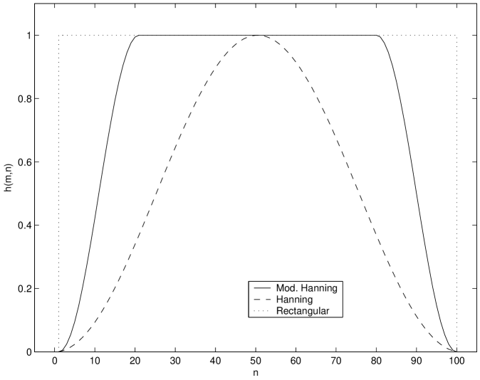
Vio et al. (2003b) show that a remarkable reduction of the edge effects in deblurring operations, that causes little distortion in the final result, can be obtained if, instead of $\boldsymbol{g}$, we use $\boldsymbol{o}=\boldsymbol{g}\,\cdot\boldsymbol{h}$ (“$\leavevmode\nobreak\ \cdot\leavevmode\nobreak\$” denotes element wise multiplication) and $\boldsymbol{h}$ is a modification of the classical Hanning window

$$h(m,n)=\left\{\begin{array}[]{ll}0.25\times\alpha\times\beta,&0\leq m,n<N_{w};\\ 0.25\times\alpha\times\beta,&N-N_{w}\leq m,n<N;\\ 1&{\rm otherwise}.\end{array}\right.$$ (14)

The parameters $\alpha=[1-\cos(m\pi/N_{w})]$ and $\beta=[1-\cos(n\pi/N_{w})]$ are chosen so that the pixels in the central subimage are not modified and the image has continuous first derivatives at the edges (see Fig. 2). This window approaches the classical two-dimensional Hanning window as $N_{w}\rightarrow N/2$ and tends to the rectangular window as $N_{w}\rightarrow 0$. The parameter $N_{w}$ thus determines the filtering characteristics, in particular the frequency pass-band, of the window. Its “optimal” value depends on many factors such as the noise level, the form of the PSF and the specific realization of the process. For a Gaussian PSF, simulation results (Vio et al. 2003b) show that values of three or four times the dispersion of the PSF provide reasonably good results. The only unavoidable consequence of the procedure is that a border of thickness $N_{w}$ has to be removed from the final deblurred image.

According to these results, $\hat{o}(m,n)$ should permit the use of (12) also in situations where the circulant approximation for the blurring operator is not appropriate. We test this via numerical simulations.

5 Some numerical experiments

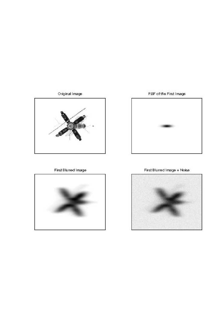
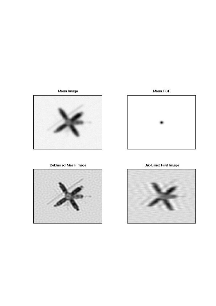
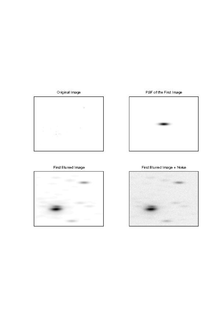
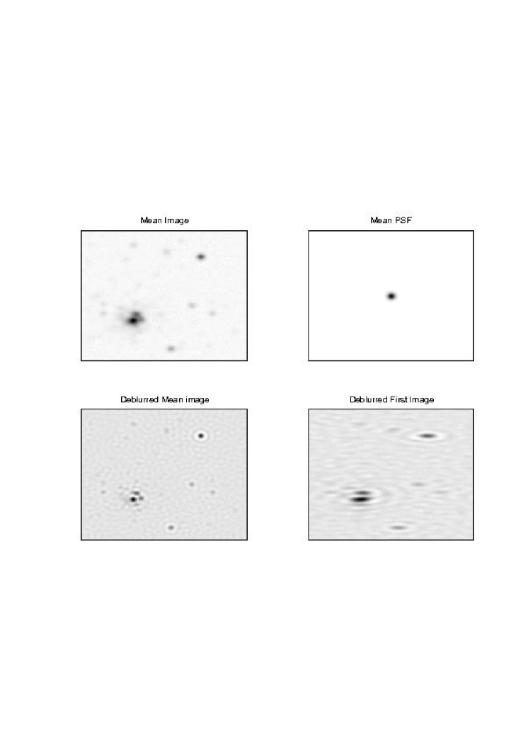
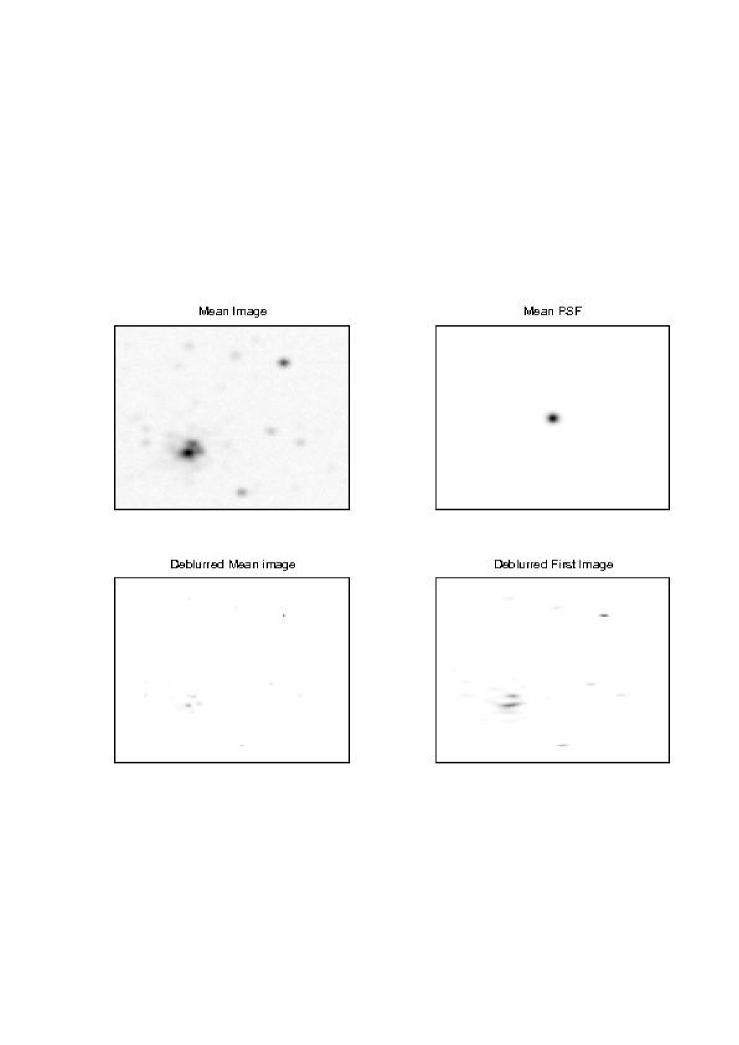
We present the results of some numerical simulations to show the flexibility and reliability of the methodology presented above. Figs. 3-8 show the deblurring results for an extended object and a set of point-like objects. We have chosen these particular examples since, being non-smooth functions, their restoration is a difficult problem. Eight images are available for each object. In each case the PSF is a bidimensional Gaussian with dispersion along the major axis set to twelve pixels, and to four pixels along the minor axis. Their inclinations take equispaced values in the range $0^{\circ}-160^{\circ}$. Gaussian white noise is added with a standard deviation of $2\%$ of the maximum value of the blurred images. Two deblurring methods have been used: a classical conjugate gradient method for LS problems (CGLS) (Björck 1996), and a modified residual norm steepest descent method (MRNSD) that can be used to enforce nonnegativity of the solution (Nagy & Strakoš 2000). For comparison, the deblurring of the first image of the set (that with the PSF with major axis inclined at $0^{\circ}$) is also shown. In every case the improvement due to the use of the eight images is evident.

Figure 6: Original image, blurred version and blurred + noise version of the first image of the set (see text) and corresponding PSF. The images are $256\times 256$ pixels.

Figure 7: Mean image $\zeta(m,n)$ and corresponding PSF for the image shown in Fig. 6, deblurred version of $\zeta(m,n)$, and deblurred version of the first image of the set (see text). The deblurring was done with CGLS. The images shown are the ones with the smallest standard deviation of the true residuals; for the mean image and the first image of the set these are $6.09\times 10^{-3}$ and $6.17\times 10^{-3}$, respectively.

Figure 8: Mean image $\zeta(m,n)$ and corresponding PSF for the image shown in Fig. 3, deblurred version of $\zeta(m,n)$, and deblurred version of the first image of the set (see text). The deblurring was done with MRNSD ($1000$ iterations). The images shown are the ones with the smallest standard deviation of the true residuals; for the mean image and the first image of the set these are $5.52\times 10^{-3}$ and $6.02\times 10^{-3}$, respectively.

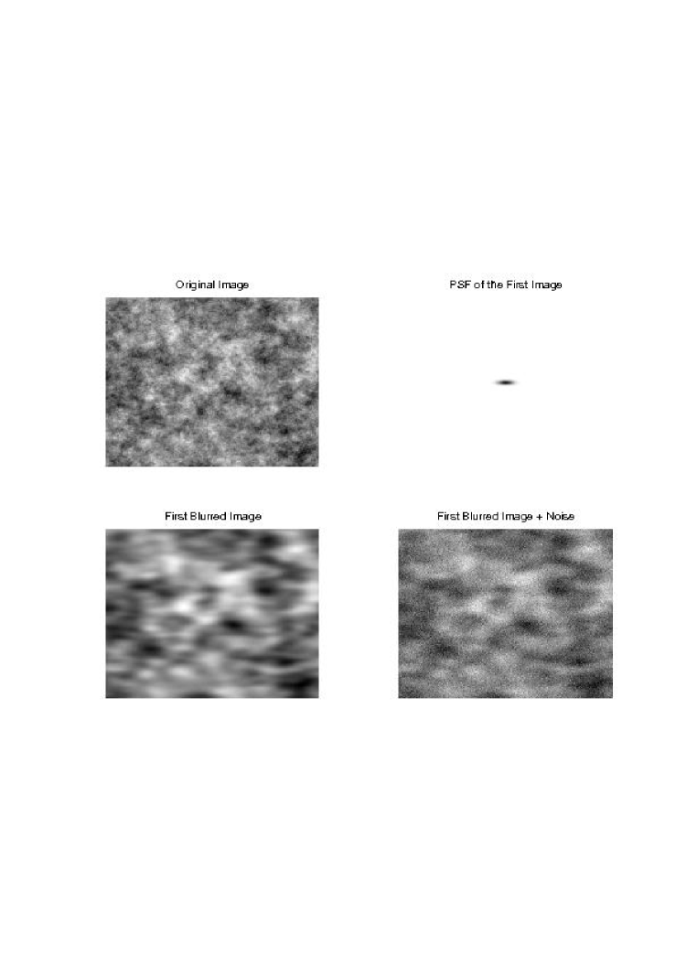
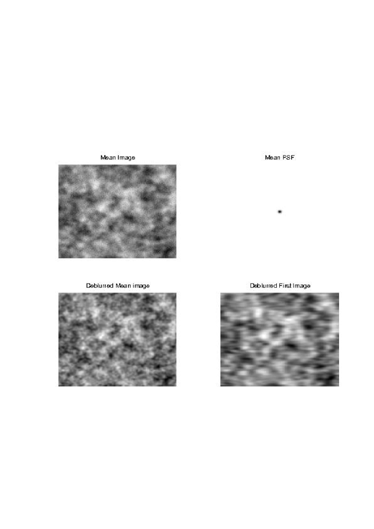
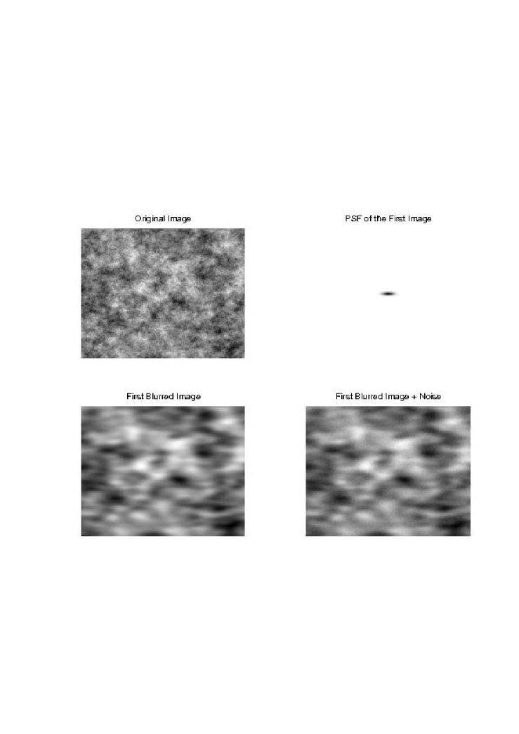
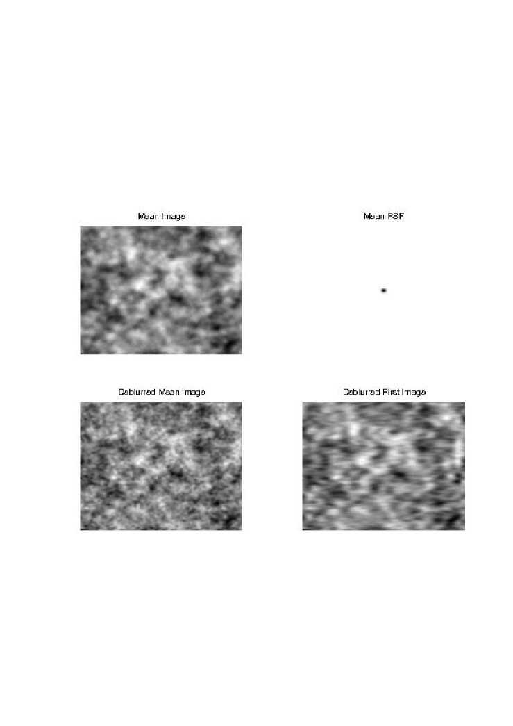
The two examples just presented do not suffer edge effects. The objects are in the center of the images and their borders show only “dark sky”. A more difficult example is provided by images with details near their borders since in this case the circulant approximation for the blurring operator is incorrect. In order to show the results obtainable in this case, we consider observations of the Cosmic Microwave Background (CMB) (e.g., see Vio et al. 2003a). Although the PSFs considered in this work are different from those typical of CMB observations, we have chosen this example because the CMB signal is expected to be the realization of a stationary stochastic process covering the whole sky. It represents one of the most unfavourable situations in the deblurring of astronomical images. Figs. 9-12 show that, despite the difficulty of the problem, the application of the windowing procedure presented in Sect. 4 can provide good results. The experiments have been carried out under the same conditions as the previous ones, with the difference that two different levels of noise have been tested ($2\%$ and $10\%$ of the dispersion of the blurred signal), and the method used in the deblurring is the classical Tikhonov approach. The CMB maps have been simulated as described in Vio et al. (2003a). Again the results are reasonably good.

Figure 9: Original image, blurred version and blurred + noise version of the first image of the set (see text) and corresponding PSF. The images are $340\times 340$ pixels. Noise of S/N = 2.

Figure 10: Mean image $\zeta(m,n)$ and corresponding PSF for the image shown in Fig. 9, deblurred version of $\zeta(m,n)$, and deblurred version of the first image of the set (see text). The deblurring was done with the classical Tikhonov method and the windowing procedure explained in the text ($N_{w}=30$ pixels). The images shown are the ones with the smallest standard deviation of the true residuals that for the mean image and the first image of the set are $0.40$ and $0.52$, respectively.

Figure 11: Original image, blurred version and blurred + noise version of the first image of the set (see text) and corresponding PSF. The images are $340\times 340$ pixels. Noise of S/N = 10.

Figure 12: Mean image $\zeta(m,n)$ and corresponding PSF for the image shown in Fig. 11, deblurred version of $\zeta(m,n)$, and deblurred version of the first image of the set (see text). The deblurring was done with the classical Tikhonov method and the windowing procedure explained in the text ($N_{w}=30$ pixels). The images shown are the ones with the smallest standard deviation of the true residuals that for the mean image and the first image of the set are $0.35$ and $0.48$, respectively.

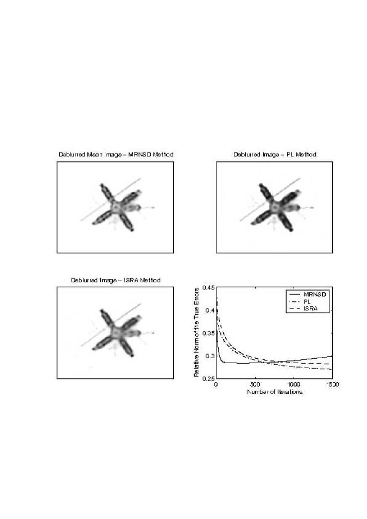
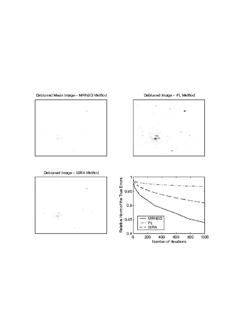
Our examples have shown that the use of $\zeta(m,n)$ coupled with standard deblurring algorithms can remarkably improve the results. However, it is still necessary to check the effective gain in computational cost. Figs. 13 and  14 show that the convergence rate of the MRNSD algorithm applied to $\zeta(m,n)$ is faster than that of the PL or ISRA methods applied to $\vartheta(m,n)$ (the cost per iteration of each method is essentially the same). We remark that MRNSD did not perform very well when applied to the more ill-conditioned problem involving $\vartheta(m,n)$. This is not too surprising since MRNSD is essentially a steepest descent method, which is known to have poorer convergence properties for more ill-conditioned problems. It has been shown in Nagy & Strakoš (2000) that preconditioning can dramatically increase the convergence rate for MRNSD, but it is a nontrivial process to choose an appropriate preconditioner, especially for severely ill-conditioned problems; see Nagy & Strakoš (2000) for further details.

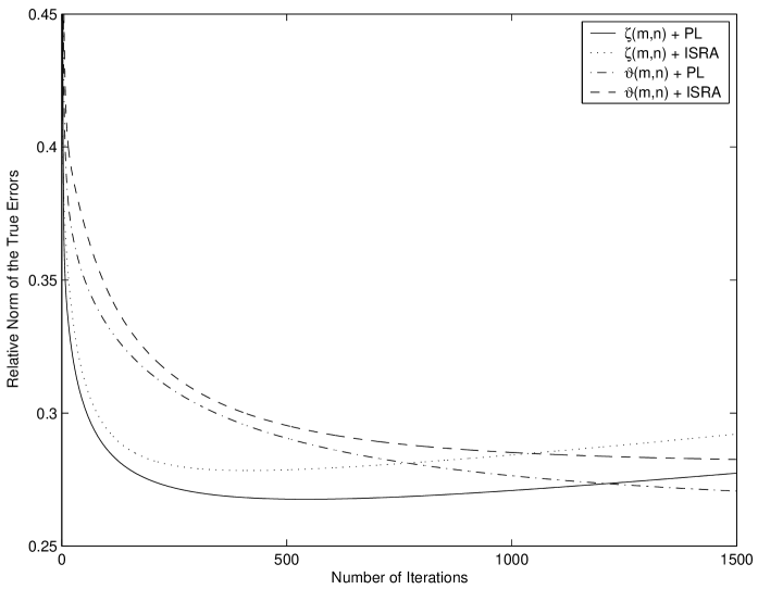
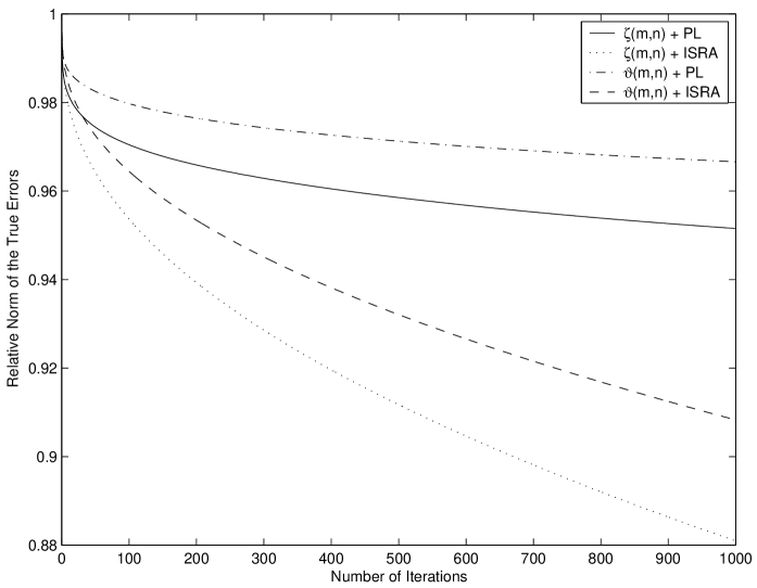
Furthermore, to check that this result is not due to the kind of algorithm used, Figs. 15, and 16 compare the convergence rate when the PL and ISRA methods are applied to both $\zeta(m,n)$ and $\vartheta(m,n)$. Again, it is evident that the use $\zeta(m,n)$ can improve the convergence rate of the algorithms.

Figure 13: Deblurred images, corresponding to the image shown in Fig. 3, obtained through the MRNSD method applied to $\zeta(m,n)$ , and the PL, and ISRA methods applied to $\vartheta(m,n)$. The images shown are the ones with the smallest standard deviation of the true residuals that are $5.92\times 10^{-2}$, $5.39\times 10^{-2}$, and $5.63\times 10^{-2}$ respectively. The convergence curves for each method is also shown: MRSND converges after $346$ iterations, whereas both PL and ISRA do not converge after $1500$ iterations.

Figure 14: Deblurred images, corresponding to the image shown in Fig. 6 obtained through the MRNSD method applied to $\zeta(m,n)$ , and the PL, and ISRA methods applied to $\vartheta(m,n)$. The images shown are the ones with the smallest standard deviation of the true residuals that are $5.52\times 10^{-3}$, $6.05\times 10^{-3}$, and $5.69\times 10^{-2}$ respectively. The convergence rate for each method is also shown: none of the methods converged before 1000 iterations.

Figure 15: Convergence rate, corresponding to the image shown in Fig. 3, for the PS and ISRA methods applied to both $\zeta(m,n)$ and $\vartheta(m,n)$.

Figure 16: Convergence rate, corresponding to the image shown in Fig. 6, for the PS and ISRA methods applied to both $\zeta(m,n)$ and $\vartheta(m,n)$.

6 Extension to images with different noise levels

So far we have assumed that the noise level is the same in all the images ($\sigma_{w_{j}}=\sigma_{w}$), a condition that allows the combination of different images to provide the most interesting results. Moreover, this requirement is often satisfied in practice. For example, with LBT the images taken at different orientations of the telescope are expected to be characterized by the same noise level.

The extension of the method to images with different noise levels is straightforward. If the different $\sigma_{w_{i}}$ are known, one may account for the different variabilities by changing equation (5) to

$$\boldsymbol{f}=\arg\min\,\sum_{j=1}^{p}\|\,(\,\boldsymbol{A}_{j}\boldsymbol{f}-\boldsymbol{g}_{j}\,)/\sigma_{w_{j}}\,\|^{2},$$ (15)

or, alternatively,

$$\boldsymbol{f}=\arg\min\,\sum_{j=1}^{p}\|\,\boldsymbol{\cal A}_{j}\boldsymbol{f}-\boldsymbol{\varrho}_{j}\,\|^{2},$$ (16)

where $\boldsymbol{\cal A}_{j}$ and $\boldsymbol{\varrho}_{j}$ represent, respectively, the matrix $\boldsymbol{A}_{j}$ and array $\boldsymbol{g}_{j}$ with their elements divided by $\sigma_{w_{j}}$. The rest of the procedure remains as described in Sect. 3. For example, Eq. (13) becomes

$$\hat{\cal K}_{j_{0}}(m,n)=\max\,[\,\hat{\cal K}_{1}(m,n),\hat{\cal K}_{2}(m,n),\ldots,\hat{\cal K}_{p}(m,n)\,],$$ (17)

where $\hat{\cal K}_{j}(m,n)=\hat{K}_{j}(m,n)/\sigma_{w_{j}}$.

7 Concluding remarks

We have considered the problem of simultaneously deblurring a set of images of a fixed object blurred by different space-invariant PSFs. Although currently available methods seem to provide good results, they are comptutationally expensive. We have developed a method, based on a LS approach, to efficiently transform a multi-image deblurring problem into a single-image one. This approach provides substantial savings in computational requirements and can be implemented using standard currently available numerical algorithms. These conclusions are confirmed by our numerical experiments.

But despite these encouraging results, some questions are still open. In particular, regularization parameter selection methods (such as GCV for the Tikhonov approach) have to be extended to deal with the correlated noise component of the mean image. This is especially important for the deblurring of random fields where the statistical properties of the field are more important than a particular realization.

Another question is the generalization of the proposed method to non-Gaussian noise. For example, for Poisson noise good results have been obtained with the maximum-likelihood estimate

$$\boldsymbol{f} =\arg\max\,\sum_{j=1}^{p}\sum_{m,n=0}^{N-1}$$

$$[\,g_{j}(m,n)\ln(\boldsymbol{A}_{j}\boldsymbol{f})(m,n)-(\boldsymbol{A}_{j}\,\boldsymbol{f})(m,n)],$$ (18)

(Correia & Richichi 2000; Bertero & Boccacci 2000a).

Appendix A Multi-Frame Deblurring and Weighted Least-Squares

In this appendix the multi-frame deblurring problem presented in the previous sections is shown to be related to (column) weighted LS.

In the multi-frame deblurring problem, we consider the LS problem (we omit regularization, but this can be easily incorporated into the discussion):

$$\min\left\|\left[\begin{array}[]{c}\boldsymbol{A}_{1}\\ \boldsymbol{A}_{2}\\ \vdots\\ \boldsymbol{A}_{p}\end{array}\right]\boldsymbol{f}-\left[\begin{array}[]{c}\boldsymbol{g}_{1}\\ \boldsymbol{g}_{2}\\ \vdots\\ \boldsymbol{g}_{p}\end{array}\right]\right\|_{2}$$ (19)

Assuming each $\boldsymbol{A}_{j}$ is block circulant, and can be diagonalized by the unitary Fourier transform matrix, then this problem can be transformed to the equivalent LS problem:

$$\min\left\|\left[\begin{array}[]{c}\boldsymbol{\Lambda}_{1}\\ \boldsymbol{\Lambda}_{2}\\ \vdots\\ \boldsymbol{\Lambda}_{p}\end{array}\right]\boldsymbol{\hat{f}}-\left[\begin{array}[]{c}\boldsymbol{\hat{g}}_{1}\\ \boldsymbol{\hat{g}}_{2}\\ \vdots\\ \boldsymbol{\hat{g}}_{p}\end{array}\right]\right\|_{2}$$ (20)

where $\boldsymbol{\Lambda}_{j}=\mbox{diag}(\lambda_{1}^{(j)},\lambda_{2}^{(j)},\ldots,\lambda_{N}^{(j)})$ is a diagonal matrix containing the eigenvalues of the matrix $\boldsymbol{A}_{j}$ (i.e., this is just the DFT of the PSF, or in the notation of the main text $\boldsymbol{\hat{K}}_{j}$).

Now, following the arguments in Sect. 3, let $\displaystyle\delta_{i}=\max_{1\leq j\leq p}\{\lambda_{i}^{(j)}\}\,,$ $i=1,2,\ldots,N$. Define the diagonal matrix:

$$\boldsymbol{\Delta}=\mbox{diag}(\delta_{1},\delta_{2},\ldots,\delta_{N})\,,$$ (21)

and consider the (column) weighted LS problem:

$$\min\left\|\left[\begin{array}[]{c}\boldsymbol{\Lambda}_{1}\boldsymbol{\Delta}^{-1}\\ \boldsymbol{\Lambda}_{2}\boldsymbol{\Delta}^{-1}\\ \vdots\\ \boldsymbol{\Lambda}_{p}\boldsymbol{\Delta}^{-1}\end{array}\right]\boldsymbol{\Delta}\boldsymbol{\hat{f}}-\left[\begin{array}[]{c}\boldsymbol{\hat{g}}_{1}\\ \boldsymbol{\hat{g}}_{2}\\ \vdots\\ \boldsymbol{\hat{g}}_{p}\end{array}\right]\right\|_{2}$$ (22)

We will write this LS problem as:

$$\min||\,\boldsymbol{D}\boldsymbol{\Delta}\boldsymbol{\hat{f}}-\boldsymbol{\hat{g}}\,||_{2}\,,$$ (23)

where

$$\boldsymbol{D}=\left[\begin{array}[]{c}\boldsymbol{\Lambda}_{1}\boldsymbol{\Delta}^{-1}\\ \boldsymbol{\Lambda}_{2}\boldsymbol{\Delta}^{-1}\\ \vdots\\ \boldsymbol{\Lambda}_{p}\boldsymbol{\Delta}^{-1}\end{array}\right]\,.$$ (24)

The normal equations version of this LS problem is:

$$\boldsymbol{\Delta}^{*}\boldsymbol{D}^{*}\boldsymbol{D}\Delta\boldsymbol{\hat{f}}=\boldsymbol{\Delta}^{*}\boldsymbol{D}^{*}\boldsymbol{\hat{g}}\,,$$ (25)

or, equivalently,

$$\boldsymbol{D}^{*}\boldsymbol{D}\boldsymbol{\Delta}\boldsymbol{\hat{f}}=\boldsymbol{D}^{*}\boldsymbol{\hat{g}}\,,$$ (26)

where $\boldsymbol{D}^{*}$ is the complex conjugate transpose of $\boldsymbol{D}$.

Now, observe that $\boldsymbol{D}^{*}\boldsymbol{D}$ is perfectly well conditioned, and thus can be easily inverted. To see this, note that for all $i$, there exists $j_{0}=j_{0}(i)$ such that

$$\delta_{i}=\lambda_{i}^{(j_{0})}\,,\quad\mbox{and}\quad|\,\lambda_{i}^{(j_{0})}\,|\geq|\,\lambda_{i}^{(j)}\,|\,,\;j\neq j_{0}\,.$$ (27)

The $i$th diagonal entry of $\boldsymbol{D}^{*}\boldsymbol{D}$ is

$$\sum_{j=1}^{p}\frac{|\,\lambda_{i}^{(j)}\,|^{2}}{|\,\delta_{i}\,|^{2}}=1+\sum_{j\neq j_{0}}\frac{|\,\lambda_{i}^{(j)}\,|^{2}}{|\,\lambda_{i}^{(j_{0})}\,|^{2}}$$ (28)

and thus each diagonal entry of $\boldsymbol{D}^{*}\boldsymbol{D}$ can be bounded by

$$1\leq\sum_{j=1}^{p}\frac{|\,\lambda_{i}^{(j)}\,|^{2}}{|\,\delta_{i}\,|^{2}}\leq p\,.$$ (29)

Thus $\boldsymbol{D}^{*}\boldsymbol{D}$ is perfectly well conditioned.

Since $\boldsymbol{D}^{*}\boldsymbol{D}$ is perfectly well conditioned, there is no danger in transforming the normal equations given in equation (26) to

$$\boldsymbol{\Delta}\boldsymbol{\hat{f}}=(\boldsymbol{D}^{*}\boldsymbol{D})^{-1}\boldsymbol{D}^{*}\boldsymbol{\hat{g}}\,,$$ (30)

which is equivalent to Eq. (12).

A vast literature is available on column weighted LS; see, for example, Golub & Van Loan (1996), Lawson & Hanson (1995), and Björck (1996).

References

- Angel et al. (1998) Angel, J.R.P., Hill, J.M., Strittmatter, P.A., Salinari, P., & Weigelt, G., 1998, in: Astronomical Interferometry, eds., R.D. Reasenberg, Proc. SPIE, 3352, 881
- Bertero & Boccacci (2000a) Bertero, M., & Boccacci, P., 2000, A&A, 144, 181
- Bertero & Boccacci (2000b) Bertero, M., & Boccacci, P., 2000, A&A, 147, 323
- Correia & Richichi (2000) Correia, s. & Richichi, A. 2000, A&A, 141, 201
- Björck (1996) Björck, Å 1996, Numerical Methods for Least Squares Problems (SIAM, Philadelphia) IEEE Trans. Med. Im. 5, 61
- Golub & Van Loan (1996) Golub, G.H., & Van Loan, C. 1996, Matrix Computations, third edition (Johns Hopkins Press, London)
- Lawson & Hanson (1995) Lawson, C.L., & Hanson, R.J, 1995, Solving Least Squares Problems (SIAM, Philadelphia)
- Lee et al. (2002) Lee, K.P., Nagy, J.G., & Perrone, L., 2002, Iterative Methods for Image Restoration: A Matlab Object Oriented Approach
- Nagy & Strakoš (2000) Nagy, J.G., & Strakoš, Z., 2000, Mathematical Modeling, Estimation, and Imaging, Wilson et. al., eds., SPIE, volume 3461, 182, 190.
- Stolyarov et al. (2002) Stolyarov, V., Hobson, M.P., Ashdown,, M.A.J., & Lasenby, A.N. 2002, MNRAS, 336, 97
- Tegmark (1999) Tegmark, M. 1999, ApJ, 519, 513
- Vio et al. (2003a) Vio, R., Nagy, J., Tenorio, L., et al. 2003, A&A, 389, 404
- Vio et al. (2003b) Vio, R., Nagy, J., Tenorio, L., et al. 2003, A&A, in press
- Vogel (2002) Vogel, C. R. 2002, Computational Methods for Inverse Problems, Ser. in Front. in Appl. Math., Vol.24, (SIAM, Philadelphia)