Self-Gravitating Eccentric Disk Models for the Double Nucleus of M31

Abstract

We present new dynamical models of weakly self-gravitating, finite dispersion eccentric stellar disks around central black holes for the double nucleus of M31. The disk is fixed in a frame rotating at constant precession speed, and is populated by stars on quasi-periodic orbits whose parents are numerically integrated periodic orbits in the total potential. A distribution of quasi-periodic orbits about a given parent is approximated by a distribution of Kepler orbits dispersed in eccentricity and orientation, using an approximate phase-space distribution function written in terms of the integrals of motion in the Kepler problem. We use these models, along with an optimization routine, to fit available published kinematics and photometry in the inner $2\hbox{${}^{\prime\prime}$}$ of the nucleus. A grid of 24 best-fit models is computed to accurately constrain the mass of the central black hole and nuclear disk parameters. We find that the supermassive black hole in M31 has mass $M_{BH}=5.62\pm 0.66\times 10^{7}\mbox{$\,M_{\odot}$}$, which is consistent with the observed correlation between the central black hole mass and the velocity dispersion of its host spheroid. Our models precess rapidly, at $\Omega=36.5\pm 4.2\mbox{$\rm\,km\,s^{-1}pc^{-1}$}$, and possess a characteristic radial eccentricity distribution, which gives rise to multi-modal line of sight velocity distributions along lines of sight near the black hole. These features can be used as sensitive discriminants of disk structure.

1 Introduction

It is widely believed that most, if not all, galaxies have supermassive black holes (BHs) in their centers. Estimates of the total mass density in quasar remnants (Soltan 1982, Chokshi & Turner 1992), models for the evolution of the quasar luminosity function in hierarchical structure formation scenarios (Haehnelt & Rees 1993), and the large numbers of nearby galaxies with low-luminosity nuclear activity (Ho, Filippenko & Sargent 1997) are consistent with this belief, assuming that active galactic nuclei (AGNs) are powered by accretion of matter onto a BH (Lynden-Bell 1969, Rees 1984).

The discovery that the BH mass ($M_{BH}$) correlates with certain host galaxy properties has made obtaining accurate masses for these objects a high priority in extragalactic studies. Kormendy & Richstone (1995) and Magorrian et al. (1998) find that BH mass is proportional to the mass or luminosity of the host spheroidal component, though with significant scatter. Ferrarese & Merritt (2000) and Gebhardt et al. (2000a) find that the BH mass correlates with the velocity dispersion ($\sigma$) of the stellar component, with much less scatter than the previous correlation; from a sample of 31 galaxies with secure BH mass estimates, Tremaine et al. (2002) find that the correlation can be written as $\log(M_{BH}/\mbox{$\,M_{\odot}$})=\alpha+\beta\log(\sigma/\sigma_{0})$, where $\alpha=8.13\pm 0.06$ and $\beta=4.02\pm 0.32$ for a reference dispersion of $\sigma_{0}=200\mbox{${\rm\,km\,s}^{-1}$}$. Since $\sigma$ is measured outside the radius of influence of the BH, defined to be $r_{h}=GM_{BH}/\sigma^{2}$, the $M_{BH}$ - $\sigma$ correlation demonstrates a fundamental relationship between the BH and its host spheroid. Such a correlation has important implications for theories of BH and galaxy formation and evolution. It is thus important to confirm and strengthen the correlation by providing highly accurate BH masses for a large number of galaxies.

BH masses can be found using a variety of techniques, including: measuring the kinematics of individually resolved stars (Eckart & Genzel 1996, Ghez et al. 1998, Schödel et al. 2002, Ghez et al. 2003), dynamical modeling of spatially resolved stellar absorption-line kinematics near the BH (see Kormendy & Richstone 1995, Verolme et al. 2002, Gebhardt et al. 2003), measuring rotation curves from optical (Harms et al. 1994, Macchetto et al. 1997, Bower et al. 1998, van der Marel & van den Bosch 1998, Marconi et al. 2003) or maser (Miyoshi et al. 1995, Ishihara et al. 2001) emission lines from orbiting gas, reverberation mapping in active galaxies (Peterson & Wandel 1999, Peterson & Wandel 2000, Gebhardt et al. 2000b), and modeling of line profile widths (Vestergaard 2002). The kinematics of resolved stellar motions and small maser disks provide the most reliable mass estimates. However, the motions of individual stars can only be resolved in the Milky Way (see Schödel et al. 2002), and regular maser emission is only found in a few galaxies (Hagiwara et al. 2003). Of the other techniques, stellar-dynamical modeling provides the most secure BH measurements; gas near the BH can be subject to non-gravitational forces, unlike the stellar component.

The kinematic data must be resolved inside the region where Keplerian motion dominates, however, to ensure that those stars fully contribute to the line of sight velocity distribution (LOSVD), and not just in its tails. Simple calculations suggest that Keplerian motion should dominate within a region of radius $r_{k}=kr_{h}$, where $k\approx 0.1$ - $0.3$, depending on the BH mass and stellar radial density profile. Using $k=0.3$, it is easy to show that $r_{k}\leq 1.3\times 10^{-3}M_{BH}/\sigma^{2}$ (pc), with $M_{BH}$ in solar masses and $\sigma$ in km/s. Using values for $M_{BH}$, $\sigma$, and distance given in Tremaine et al. (2002), or from the $M_{BH}$ - $\sigma$ relation, $r_{k}$ subtends an angle of $11\hbox{$.\!\!^{\prime\prime}$}60$, $0\hbox{$.\!\!^{\prime\prime}$}74$, and $0\hbox{$.\!\!^{\prime\prime}$}15$ for the Milky Way, M31, and M32, respectively. Other than the Milky Way, M31 is the only nearby galaxy in the Local Group with a resolved $r_{k}$ at the resolution of the Hubble Space Telescope (HST) Space Telescope Imaging Spectrograph (STIS; $\sim 0\hbox{$.\!\!^{\prime\prime}$}1$); M33 is consistent with having a maximum BH mass of $\sim 3000\mbox{$\,M_{\odot}$}$ (Merritt et al. 2001, Gebhardt et al. 2001), so its $r_{k}$ subtends an angle $<0\hbox{$.\!\!^{\prime\prime}$}005$.

M31 offers a unique opportunity to obtain a secure BH mass from spatially resolved stellar kinematics inside $r_{k}$. M31 is also the nearest galaxy with a normal bulge (Kormendy 1993), and it has a nucleus; that is, a small-scale stellar component which is photometrically and dynamically distinct from the bulge and the large-scale galactic disk (Kormendy & Richstone 1995, and references therein). Galaxy nuclei are poorly understood, as is the dynamical connection between the nuclear stars and the central BH. M31’s nucleus is $\sim 2\hbox{${}^{\prime\prime}$}$ in radius (Light, Danielson & Schwarzschild 1974), which is fully within the sphere of influence of the BH; $r_{h}\simeq 2\hbox{$.\!\!^{\prime\prime}$}5$, if M31 is located at a distance of $770$ kpc and has a BH mass of $5.5\times 10^{7}\mbox{$\,M_{\odot}$}$, as implied by the $M_{BH}$ - $\sigma$ relation. Thus, M31’s nucleus allows for a more detailed dynamical study than is possible for any other galaxy. Even more enticing is the fact that the nucleus is shown to be double; the photometric profile shows two brightness peaks, one of which is off-center with respect to the outer bulge isophotes. Kinematic profiles also show strong asymmetries. Thus, standard axisymmetric dynamical modeling techniques (e.g. in Gebhardt et al. 2003) are inappropriate. New modeling methods are needed to obtain an accurate measure the BH mass in M31.

M31 was first shown to have a photometrically asymmetric nucleus by Light et al. (1974), using the Stratoscope II balloon-borne telescope. Nieto et al. (1986) confirmed those observations with groundbased data, and found that the brightest point in the nucleus was offset from the center of the bulge by $\sim 0\hbox{$.\!\!^{\prime\prime}$}4$. The HST Wide-field and Planetary Camera (WFPC1) later resolved the nucleus into two brightness peaks (Lauer et al. 1993, hereafter L93), as did more recent HST images taken with WFPC2 (Lauer et al. 1998, hereafter L98). The optically brighter peak, P1, is offset $0\hbox{$.\!\!^{\prime\prime}$}49$ from the bulge photometric center, which coincides with the fainter peak, P2. P1 and P2 have central $V$ band surface brightnesses of $13.4\mbox{${\rm\,mag\,arcsec}^{-2}$}$ and $13.7\mbox{${\rm\,mag\,arcsec}^{-2}$}$, respectively, when averaged over a $0\hbox{$.\!\!^{\prime\prime}$}22$ wide slit (L93). P1 is compact, with a major-axis core radius of $\sim 0\hbox{$.\!\!^{\prime\prime}$}4$; P2 has a weak stellar cusp, unlike P1 (L93).

Near-IR (Mould et al. 1989, Davidge et al. 1997, Corbin et al. 2001), optical (L93, L98), and far-UV (King et al. 1995, hereafter K95) images all show that the asymmetric or double-peaked structure of the nucleus is not caused by dust absorption. Along with absorption-line strengths from long-slit spectra (Kormendy & Bender 1999, hereafter KB99), they also demonstrate that P1 has a similar stellar content as the rest of the nucleus, which is unlike any globular cluster or dwarf elliptical. Thus, P1 is an intrinsic part of the nucleus, and not an interloping star cluster (K95). The $V-I$ color of the nucleus is not the same as that of the bulge, implying a difference in stellar populations (L98, Bacon et al. 2001, hereafter B01); line strengths in KB99 also show the same. The color difference is not agreed upon, however; L98 find that the nucleus is redder than the bulge, whereas B01 find the opposite. Sil’chenko et al. (1998) argue that the nucleus is more metal rich than the bulge, and, using $H_{\beta}$ lines to disentangle metallicity and age, find that the nucleus is a factor of three younger than the bulge.

P2 is brighter than P1 in the UV, as a result of an embedded UV-bright source (hereafter the UV peak; K95, Brown et al. 1998, L98) whose center is located $0\hbox{$.\!\!^{\prime\prime}$}076$ toward P1 from the center of P2 in the $I$-band (B01). The UV peak is resolved, with a half-power radius of $\sim 0\hbox{$.\!\!^{\prime\prime}$}2$ (Brown et al. 1998, L98, B01). Brown et al. (1998) show that the UV peak is consistent with being comprised of extreme horizontal branch stars with masses between $0.47$ and $0.53$ $\,M_{\odot}$, but not consistent with a majority contribution from main sequence stars, blue stragglers, or post-asymptotic giant branch stars more massive than $0.56\mbox{$\,M_{\odot}$}$. Unpublished spectra from STIS also suggest that the UV peak is dominated by starlight (E. Emsellem, private communication), rather than a low-level AGN (K95). The UV peak is thought to be the location of the photometric center of the bulge, and the supermassive BH (K95, KB99, B01; Peng 2002, hereafter P02). Hereafter in this paper, “the nucleus” refers to P1 and P2 together, but does not include the UV peak, which is a separate nuclear star cluster. The locations of P1, P2, and the UV peak with respect to the nucleus as a whole are shown in Figure 1.

Figure 1: WFPC2/HST photometry in the $I$ (F814W) band from L98. The image has been boxcar smoothed for clarity. North points toward the top of the page, while East points to the left. Arrows show the locations of P1, P2, and the UV peak; the center of the UV peak is denoted by an asterisk at the origin. The solid line shows the P1-P2 line (PA${}_{d}=42\hbox{${}^{\circ}$}$), or the major axis of the nucleus. The dotted line shows the kinematic major axis, which is the line joining the velocity extrema in the two-dimensional kinematic map (PA${}_{K}=56.4\hbox{${}^{\circ}$}$).

Groundbased observations at $\sim 1\hbox{${}^{\prime\prime}$}$ (FWHM) resolution by Dressler (1984), Kormendy (1988), Dressler & Richstone (1988), and van der Marel et al. (1994) were the first to show that the stellar component in M31’s nucleus rotates rapidly, and that there is a significant velocity dispersion peak (hereafter the dispersion spike) in the central few parsecs, both possibly indicating the presence of a central BH of mass $\sim 10^{7}\mbox{$\,M_{\odot}$}$. The data show the dispersion spike to be centered $\sim 0\hbox{$.\!\!^{\prime\prime}$}6$ away from the peak in brightness (P1) in the Stratoscope II photometry, and the nucleus to be colder than the bulge on both sides of the dynamical center. Two-dimensional kinematic maps obtained by Bacon et al. (1994) at similar resolution ($0\hbox{$.\!\!^{\prime\prime}$}87$ FWHM), using the TIGER integral field spectrograph on the Canada-France-Hawaii Telescope (CFHT), are consistent with most of the earlier observations; however, the dispersion spike in that data set is located $\sim 0\hbox{$.\!\!^{\prime\prime}$}7$ from P2 on the anti-P1 side of the nucleus, which places it $\sim 0\hbox{$.\!\!^{\prime\prime}$}6$ farther away from P1 than found previously. The deconvolved TIGER rotation curve is asymmetric about the rotation center, which is near P2; the maximum amplitude on the anti-P1 side is roughly $60\mbox{${\rm\,km\,s}^{-1}$}$ greater than that on the P1 side.

Observations at better spatial resolution ($0\hbox{$.\!\!^{\prime\prime}$}64$ FWHM) and higher signal-to-noise (S/N), taken with the Subarcsecond Imaging Spectrograph (SIS) on CFHT (KB99), show the dispersion spike offset from the UV peak by $\sim 0\hbox{$.\!\!^{\prime\prime}$}2$, roughly $0\hbox{$.\!\!^{\prime\prime}$}4$ less than the Bacon et al. (1994) offset; the spike’s amplitude is $248\pm 5\mbox{${\rm\,km\,s}^{-1}$}$ before bulge subtraction and $287\pm 9\mbox{${\rm\,km\,s}^{-1}$}$ after. The nucleus is cold on both sides of the UV peak, as in Kormendy (1988); for example, the dispersion at $r=0\hbox{$.\!\!^{\prime\prime}$}92$ from the UV peak on the P1 side is $123\pm 2\mbox{${\rm\,km\,s}^{-1}$}$ with the bulge, and $\sim 100\mbox{${\rm\,km\,s}^{-1}$}$ without. KB99 find that the bulge-subtracted maximum rotation velocity is $-236\pm 4\mbox{${\rm\,km\,s}^{-1}$}$ on the anti-P1 side, but only $179\pm 2\mbox{${\rm\,km\,s}^{-1}$}$ on the P1 side, confirming the $\sim 60\mbox{${\rm\,km\,s}^{-1}$}$ rotation amplitude asymmetry of Bacon et al. (1994). When the bulge is added, the asymmetry is only $\sim 7\mbox{${\rm\,km\,s}^{-1}$}$, with a maximum velocity on the P1 side of $152\pm 3\mbox{${\rm\,km\,s}^{-1}$}$. The zero velocity crossing is displaced from the UV peak toward P1 by $0\hbox{$.\!\!^{\prime\prime}$}051\pm 0\hbox{$.\!\!^{\prime\prime}$}014$. Slit-averaged velocity profiles from the OASIS integral field spectrograph on CFHT (B01), which has about twice the spatial resolution ($\sim 0\hbox{$.\!\!^{\prime\prime}$}4$ - $0\hbox{$.\!\!^{\prime\prime}$}5$ FWHM) as TIGER, are consistent with the SIS observations. B01 measure the kinematic major axis, or the line joining the velocity extrema in the two-dimensional map, to be at position angle PA${}_{K}=56.4\hbox{${}^{\circ}$}\pm 0.2\hbox{${}^{\circ}$}$, which is not on the P1-P2 line (PA${}_{d}=42\hbox{${}^{\circ}$}$; see Figure 1).

The kinematic observations with the best resolution to date ($\sim 0\hbox{$.\!\!^{\prime\prime}$}1$ FWHM) come from the f/48 long-slit spectrograph of the HST Faint Object Camera (FOC; Statler et al. 1999). The rotation curve is resolved through the rotation center with a projected velocity gradient of $\sim 300\mbox{$\rm\,km\,s^{-1}pc^{-1}$}$; the zero velocity crossing is offset by $0\hbox{$.\!\!^{\prime\prime}$}16\pm 0\hbox{$.\!\!^{\prime\prime}$}05$ from P2 towards P1, or $\sim 0\hbox{$.\!\!^{\prime\prime}$}135$ from the UV peak (using the spatial registration suggested by B01). The rotation curve is asymmetric, as in the SIS data, with an amplitude asymmetry of at least $60\mbox{${\rm\,km\,s}^{-1}$}$ and a P1-side maximum of $\sim 240\mbox{${\rm\,km\,s}^{-1}$}$. The dispersion spike has amplitude $440\pm 70\mbox{${\rm\,km\,s}^{-1}$}$, but is only offset from P2 by $0\hbox{$.\!\!^{\prime\prime}$}06$, in contrast to the $\sim 0\hbox{$.\!\!^{\prime\prime}$}2$ offset found with SIS and OASIS. High-resolution kinematic data from STIS/HST (B01) also show similar asymmetries. The rotation curve has an amplitude asymmetry possibly as high as $\sim 90\mbox{${\rm\,km\,s}^{-1}$}$, with a maximum rotation amplitude on the P1-side of $201\pm 5\mbox{${\rm\,km\,s}^{-1}$}$. The velocity gradient is $\sim 220\mbox{$\rm\,km\,s^{-1}pc^{-1}$}$ through the zero velocity crossing, which occurs $0\hbox{$.\!\!^{\prime\prime}$}09$ from the UV peak; both of these values are lower than for FOC. The dispersion spike has amplitude $321\pm 33\mbox{${\rm\,km\,s}^{-1}$}$, and is located $0\hbox{$.\!\!^{\prime\prime}$}235$ from the UV peak on the anti-P1 side. B01’s STIS dispersion spike is substantially more offset than that in the FOC data. We refer the reader forward to figures in Section 4.1 to see FOC, STIS, SIS and OASIS kinematic profiles.

Two hypotheses have been explored to account for the photometric and kinematic asymmetries observed in M31’s nucleus: first, that P1 represents a captured star cluster orbiting around a stellar disk and central BH (Emsellem & Combes 1997); second, that P1 is produced by orbit crowding at apoapsis in an eccentric disk of stars on apse-aligned Kepler orbits about a BH at P2 (Tremaine 1995, hereafter T95). Of the two hypotheses, the evidence strongly points toward the second as correct. The eccentric disk picture naturally explains the nearly uniform colors of the nucleus, since P1 and P2 are the same stellar population. It is difficult to explain the colors with the orbiting cluster picture, since the colors of P1 are unlike any globular cluster or dwarf elliptical. A further strike against the cluster picture is demonstrated in self-consistent N-body simulations by Emsellem & Combes (1997); they find that the timescale for disruption is only $\sim 10^{5}$ years, so it is unlikely that such a configuration would be observed.

T95’s original model for an eccentric nuclear disk in M31 consists of three nested and aligned Keplerian ringlets with outwardly decreasing eccentricities. Random velocities are roughly accounted for by convolution with a Gaussian point spread function in the plane of the sky. The model fits the photometry of L93 and is broadly consistent with the ground-based kinematics of Kormendy (1988) and Bacon et al. (1994). Though simple, the model predicts many of the asymmetries seen in the more recent kinematic profiles from SIS, FOC, STIS, and OASIS, including the displaced rotation center, the asymmetric rotation amplitudes, the low velocity dispersion at $r\sim 1\hbox{${}^{\prime\prime}$}$ on the P1 side of the nucleus, and the presence of a dispersion spike near P2.

In its original form, the T95 model is too limited to be used to constrain the mass of the central BH in M31. The model ignores self-gravity, which is necessary to maintain apse-alignment in the disk against differential precession (T95; Statler 1999, hereafter S99). Also, the model does not include a realistic treatment of velocity disperison, which is needed for an accurate prediction of the dispersion profile. Both of these ingredients need to be included self-consistently.

Hints at how such a model can be constructed were first given by Sridhar & Touma (1999). They compute orbits in nearly-Keplerian potentials with lopsided perturbations and find a family of periodic loop orbits elongated in the same sense as the perturbation. They suggest that the nearly elliptical periodic parents of such orbits can be used as the backbone around which an eccentric disk with self-gravity and finite dispersion can be built. S99 computes periodic loop orbits for a continuous, uniformly precessing T95-like disk model, and shows that the requirement of uniform precession has important consequences for the disk structure. He finds that the periodic orbits follow a non-monotonic radial eccentricity distribution, in which a steep negative eccentricity gradient though the densest part of the disk is followed by a reversal of the arrangement of pericenter and apocenter with respect to the BH. S99 suggests that approximate self-consistent equilibria can be constructed around such a sequence of numerically integrated closed periodic orbits, by approximating a distribution of quasi-periodic orbits about a given periodic parent with a distribution of Kepler orbits dispersed in eccentricity and orientation. Salow & Statler (2001) use this approximation to construct radially truncated models that reproduce many of the features seen in FOC kinematics and one-dimensional HST photometry within $0\hbox{$.\!\!^{\prime\prime}$}5$ of the UV peak; the models are built by iteration with a phase space distribution function (DF) written in terms of the integrals of motion in the Kepler problem (S99). They find that the backbone orbits follow an eccentricity distribution similar to that in S99, which gives rise to distinctive multi-peaked LOSVDs near the UV peak.

Several authors have constructed self-consistent eccentric disk models by other methods. Jalali & Rafiee (2001) construct integrable models whose potentials are of the Stäckel form in elliptic coordinates. They show that models with double nuclei are sustained by four general types of regular orbits (butterflies, nucleophilic bananas, horseshoes, and aligned loops). Their models, however, require that both P1 and P2 have density cusps, which is not seen in the data. B01 and Jacobs & Sellwood (2001) perform N-body simulations of lopsided ($m=1$) modes in a cold disk orbiting a central BH, and are able to find models that reproduce some of the observed features of the nucleus. More importantly, they demonstrate that lopsided stellar disks can be long-lived, giving further support to the eccentric disk picture. Sambhus & Sridhar (2002, hereafter SS02) construct models using a Schwarzschild-type method (Schwarzschild 1979) with an orbit library composed of both prograde and retrograde orbits. They find that the latter are needed to better fit the kinematics and photometry near P2; Touma (2002) argues that a small percentage of retrograde orbits is all that is needed for a Keplerian disk to grow an unstable lopsided mode. Both SS02 and B01 find an eccentricity distribution different than that found by S99 and Salow & Statler (2001). Orbits follow a steep negative eccentricity gradient through the dense part of the disk, but do not switch their apoapses to the anti-P1 side of the disk afterward.

Peiris & Tremaine (2003, hereafter PT03) have recently shown how a T95-like model can be extended to three-dimensions. They construct models comprised of non-interacting Kepler orbits in the gravitational field of the BH. They draw orbital elements from a Monte-Carlo scheme, and populate the disk with a parametric DF; orbits are dispersed in eccentricity, orientation, and inclination, rather than just the first two, as in Salow & Statler (2001). Their models are able to reproduce most of the important features in HST photometry and SIS and unpublished STIS (Bender et al. 2003) kinematics within $\sim 1\hbox{${}^{\prime\prime}$}$ of the UV peak. However, their models are missing self-gravity and gravity-induced precession in the disk.

In this paper we extend the self-gravitating, finite dispersion models of Salow & Statler (2001) to include a greater radial extent, in order to rigorously model the double nucleus of M31. Along with an optimization routine, these models are used to fit FOC, STIS, and SIS one-dimensional kinematics, OASIS two-dimensional kinematics, and one and two-dimensional WFPC2/HST photometry. Best-fit disk parameters and BH masses are found for a grid of 24 models by minimizing a chi-square merit function which assesses agreement between model and data. The primary result of this paper is an accurate mass for the BH in M31. Secondarily, we present the properties of the disk that best fits the nucleus.

The plan of this paper is as follows. In Section 2, we give the details of model construction. We then provide a description of the necessary assumptions and instrument specifications needed to find models that best fit data from the nucleus of M31 in Section 3. In Section 4 we present results from a grid of 24 best-fit models for M31’s nucleus, including the BH mass in M31 and disk parameters and properties. Section 5 discusses the connection with other work. Finally, Section 6 presents some brief concluding remarks.

2 Eccentric Disk Models

2.1 Theoretical Basis

Following Sridhar & Touma (1999) and S99, we construct realistic models from sets of quasi-periodic orbits whose parents are closed periodic loops elongated in the same sense as the lopsided perturbation. The parent loops form the “backbone” of the disk, around which quasi-periodic orbits will be populated. These backbone orbits will precess and deform under the influence of the disk’s self-gravity. However, if the mass of the disk is small enough the backbone orbits will be nearly Kepler ellipses in the rotating frame. This fact, together with results from simple orbit integrations in lopsided potentials, is suggestive of a way to approximate distributions of quasi-periodic orbits about a given backbone orbit. Explorations of the orbital structure in a nearly Keplerian potential perturbed by a slowly precessing eccentric disk show that quasi-periodic orbits fill bands surrounding the backbone orbits (Statler & Salow 2000); alternatively, they can be thought of as librating about the backbone orbits in eccentricity and orientation. A natural approximation is then to describe a distribution of quasi-periodic orbits about a given backbone orbit by a distribution of Kepler orbits dispersed in eccentricity and orientation. We follow this approximation, taking it as a postulate.

To represent a distribution of Kepler orbits about a given backbone orbit we use a phase space distribution function (DF) written in terms of integrals of motion in the unperturbed Kepler potential, $f(a,e,\omega)$, where $a$ is the semimajor axis, $e$ is the eccentricity, and $\omega$ is the argument of pericenter of a Kepler orbit; i.e., $\omega$ is the direction of the Runge-Lenz vector. We have chosen a simple DF which is separable in all three variables; that is, $f(a,e,\omega)=F(a)F(e)F(\omega)$. The details of the DF are given in Section 2.2.

Models include a two-dimensional eccentric stellar disk surrounding a BH of mass $M_{BH}$. The density distribution of the disk is fixed in a frame rotating at constant angular speed $\Omega$ about the center of mass of the system, and is normalized to a total mass $m=\epsilon M_{BH}$. The black hole is located at the origin of a Cartesian coordinate system, and the disk is oriented such that its major-axis lies along the $x$ coordinate line. Models are computed on a $200\times 200$ grid with spacing $l=0.25$ in dimensionless units where $G=M_{BH}=1$. The potential of a spheroidal bulge component is not included, since its effect on the precession frequencies of Kepler orbits in the absence of the disk potential is small.

2.2 The Distribution Function

$F(e)$ and $F(\omega)$ together provide our prescription for the way dispersed Kepler ellipses are distributed about the sequence of backbone orbits. We have considered two versions of $F(e)$. The first is a Gaussian distribution of eccentricities given by

$$F(e)=\exp\left[-{[e-e_{0}(a)]^{2}\over 2{\sigma_{e}}^{2}}\right],$$ (1)

where $e_{0}(a)$ describes the sequence of backbone orbits, and the constant $\sigma_{e}$ determines the spread in eccentricity about a given backbone orbit. The second version of $F(e)$ is a Rayleigh distribution of eccentricities, and is given by

$$F(e)=|e|\exp\left[-{[e-e_{0}(a)]^{2}\over 2{\sigma_{e}}^{2}}\right],$$ (2)

where $e_{0}(a)$ and $\sigma_{e}$ have the same meaning as for the Gaussian distribution. The velocity distribution for the Gaussian form of $F(e)$ is singular at $e=0$, and thus somewhat unphysical. As a result, an extra population of circular orbits will be populated, in addition to the normal eccentric orbit population around $e_{0}(a)$. The Rayleigh form adds an extra factor of $e$ to ensure finiteness at $e=0$. For both forms of $F(e)$ we use a Gaussian distribution of orientations. F($\omega$) is given by

$$F(\omega)=\exp\left[-{\omega^{2}\over 2{\sigma_{\omega}}^{2}}\right],$$ (3)

where the constant $\sigma_{\omega}$ is the dispersion in $\omega$.

The function $F(a)$ gives the mass per unit interval of semimajor axis, and thus controls the radial mass distribution. We have chosen a form for $F(a)$ which allows variability in the strength of the central density minimum, and in the strength and width of the maximum peak in the mass distribution. $F(a)$ is described by two functions joined together, $F_{I}(a)$ and $F_{O}(a)$, which represent the inner and outer parts of the disk, respectively. We use

$$F(a)=\left\{\begin{array}[]{l@{\quad:\quad}r}F_{I}(a)&a\leq a_{max}\\ F_{O}(a)&a>a_{max},\end{array}\right.$$ (4)

where $a_{max}$ is the value of $a$ at which $F_{I}(a)$ is maximum, $F_{max}$. $F_{I}(a)$ is given by

$$F_{I}(a)=\mbox{\rm max}(a-\Delta,0)\exp\left[-{(a-a_{0})^{2}\over 2{\sigma_{a}}^{2}}\right],$$ (5)

where $\sigma_{a}$ controls the width of the inner density distribution, $\Delta$ determines the strength of the central density minimum, and $a_{0}$ sets the length scale; we set $a_{0}=2$. $F_{O}(a)$ is given by

$$F_{O}(a)=CF_{I}(a)+(1-C)F_{max}\mbox{$\rm\,sech\,$}\left[(a-a_{max})\over\sigma_{r}\right].$$ (6)

The constant $C$ has two effects on the behavior of the disk: First, it determines how much mass is distributed to the outer part of the disk, and second, it partially determines how quickly the density drops-off away from maximum for $a\geq a_{max}$. Larger values of $C$ result in weaker outer disks and steeper drop-offs in density outside of maximum. Figure 2 shows the behavior of $F(a)$ for three values of $C$.

Figure 2: The function $F(a)$, which controls the radial mass distribution. $F(a)$ is shown in model units for three values of the parameter $C$ in Equation 6, which determines how mass is distributed between the inner and outer parts of the disk. $C$ also partially determines how fast the density drops-off away from maxiumum. The solid line shows $F_{I}(a)$ for $\sigma_{a}=1$, $\Delta=1$, and $a_{0}=2$. The dotted, dash-dotted, and dashed lines show $F_{O}(a)$ when $C$ has value $0.75$, $0.5$, and $0.25$, respectively. A larger value of $C$ results in a weaker outer disk and a steeper drop-off in density outside of maximum.

The parameter $\sigma_{r}$ is used to extend the disk to the desired cutoff radius, $R_{d}$. Simple algebra shows that if $F_{O}(a)=\alpha$ at $a=R_{d}$, where $\alpha$ is some small number, then $\sigma_{r}$ is given by

$$\sigma_{r}={(R_{d}-a_{max})\over\ln({(1-C)F_{max}\over\alpha}+\sqrt{[{(1-C)F_{max}\over\alpha}]^{2}-1})}.$$ (7)

We set $\alpha={F_{max}/100}$ to ensure sufficiently small densities at $a=R_{d}$.

2.3 The Construction Scheme

A model is specified by the parameters $\epsilon$, $\Omega$, $\sigma_{e}$, $\sigma_{\omega}$, $\sigma_{a}$, $\Delta$, $C$, $a_{0}$, and $R_{d}$. Once these are given, an initial guess for $e_{0}(a)$ must be provided. We choose $e_{0}(a)={1\over 2}(1-{a\over R_{d}})$, which gives an initial density maximum at apoapsis. This choice was made because it leads to rapid convergence, but the results are insensitive to the initial guess. Following specification of $e_{0}(a)$, construction proceeds iteratively (see Salow & Statler 2001).

Construction begins by expressing the DF in terms of position and velocity using the standard Keplerian relations:

$$a=-{1\over{2E}}$$ (8)

$$e=\sqrt{1+2Eh^{2}}$$ (9)

$$\omega=\arctan{{A_{y}}\over{A_{x}}}$$ (10)

where $E={1\over 2}({v_{x}}^{2}+{v_{y}}^{2})+\Phi$ is the energy per unit mass, $\Phi=-(\sqrt{x^{2}+y^{2}})^{-1}$ is the unperturbed potential, and $h=xv_{y}-yv_{x}$ is the angular momentum per unit mass (Murray & Dermott 1999). The quantities $A_{x}=v_{y}h+x\Phi$ and $A_{y}=-(v_{x}h)+y\Phi$ are the $x$ and $y$ components of the Runge-Lenz vector, respectively. To avoid discontinuities in the DF, we allow $e$ to be negative and define $\omega$ to lie between $\pm{\pi/2}$.

The disk density $\rho(x,y)$ is found by integrating the DF over velocity at each grid point, and then normalizing the grid to total disk mass $m$. The potential of the disk is computed using Fast Fourier Transforms (FFTs) and the discrete fourier convolution theorem (see Section 2.8 of Binney & Tremaine 1987). Zero padding is used to suppress Fourier images. We use a softened point-mass kernel of one grid spacing for the Green function. The disk potential is added to the potential of the black hole to form the total potential. The total potential is rotated at frequency $\Omega$ about the center of mass to include inertial effects from the rotating frame; only Coriolis forces are included, since centrifugal terms are of order $\Omega^{2}$.

Numerical integration of the equations of motion in the rotating frame is performed to find the set of closed periodic orbits that circulate in the prograde direction and precess uniformly in the total potential. Orbits are initially launched perpendicularly from the $x$-axis, and the velocities are varied until the next $x$-axis crossing occurs with $v_{x}=0$ (S99). These will be the backbone orbits for the next iteration. To ensure that only nearly-Keplerian orbits are found, the total period and computed semiminor axis have to be within $50\%$ and $20\%$, respectively, of those values for a Kepler orbit with the same semimajor axis and eccentricity. These two conditions enable separation of higher-order resonant orbits from nearly-Keplerian orbits for a wide range of tested parameter values.

The backbone orbits are expressed as a new function $e_{0}(a)$. This is done by noting the positions where the orbit crosses the $x$-axis at positive ($x_{+}$) and negative ($x_{-}$) values of $x$. Following S99, $e$ and $a$ are determined using $e\equiv(x_{-}+x_{+})/(x_{-}-x_{+})$ and $a\equiv(x_{+}-x_{-})/2$. In some cases this is all that must be done; however, for large values of $\Omega$ the sequence of periodic orbits truncates inside $R_{d}$. When this occurs, $e_{0}(a)$ is extended out to $a=R_{d}$ using a function chosen to mimic the behavior of $e_{0}(a)$ for models with no truncation. Details of this are given in Appendix A. After extending $e_{0}(a)$, the quantity $\sigma_{r}$ in Equation 6 is updated to ensure that the disk extends out to $R_{d}$, since the physical length scale can change at each iteration (see Section 3.2). A new density distribution is then found and the aforementioned sequence continues. Iterations continue until the fractional change in the density per iteration is less than 5% everywhere and less than 1% on average.

2.4 Projecting the Model

We project two-dimensional models onto the plane of the sky. Along with inclination ($i$), two position angles in the plane of the sky must be specified to fully determine a disk’s orientation: the position angle of the major axis of the disk (PA_d) and the position angle of the line of nodes (PA_n). We refer to three coordinate systems to describe how models are projected onto the sky. The first, $(x_{s},y_{s})$, is a system on the plane of the sky for which $y_{s}$ points along position angle PA$=0\hbox{${}^{\circ}$}$. The second, $(x_{d},y_{d})$, is the system in which the disk lies with its major axis along $x_{d}$. The third system, $(x_{n},y_{n})$, is oriented such that $x_{n}$ lies along the line of nodes and $y_{n}$ is in the plane of the disk. Figure 3 shows the relationship between these three coordinate systems as seen on the plane of the sky.

Figure 3: The three coordinate systems used to construct and project a model, as seen on the plane of the sky for a disk (shown as an ellipse with $e=0.3$) inclined at $i=70\hbox{${}^{\circ}$}$ with the line of nodes at PA${}_{n}=56.4\hbox{${}^{\circ}$}$ and the disk major axis at PA${}_{d}=42\hbox{${}^{\circ}$}$. All coordinate axes have the same unprojected length. Velocity moments are projected onto $(x_{s},y_{s})$ in the sky plane, with $y_{s}$ pointing North (PA=0^∘) and $x_{s}$ pointing West. $(x_{d},y_{d})$ is the system in which the disk is constructed, with its major axis along $x_{d}$. $(x_{n},y_{n})$ is oriented such that $x_{n}$ lies along the line of nodes and $y_{n}$ is in the plane of the disk.

For computational efficiency we perform kinematical modeling using velocity moments, rather than the full LOSVD. We do, however, find LOSVDs for minimized models at specific locations, as described below in Section 2.5.

Moments of the LOSVD are found on a $200\times 200$ grid with spacing $0\hbox{$.\!\!^{\prime\prime}$}02$ in the $(x_{s},y_{s})$ system. The zeroth moment, $\rho$, is found by projecting the density distribution onto the sky directly. The first and second moments, $\rho v$ and $\rho v^{2}$, are found using the DF for the converged model. Each point in the grid is transformed to a point in the disk plane, $(x_{d},y_{d})$. At $(x_{d},y_{d})$ the DF and the Kepler relations (Equations 8, 9, and 10) are used to get the distribution of velocities $f({v_{x}}_{d},{v_{y}}_{d})$ on a $200\times 200$ velocity grid with spacing $0.075$ in units where $G=M_{BH}=1$ and $a_{0}=2$. The distribution $f({v_{x}}_{d},{v_{y}}_{d})$ is then transformed to the $(x_{n},y_{n})$ coordinate system to obtain the distribution $f({v_{x}}_{n},{v_{y}}_{n})$ on a similar velocity grid. This distribution is transformed to an inertial frame to include the $\vec{\Omega}\times\vec{r}$ contribution to the velocity, and integrated over ${v_{x}}_{n}$ to give $f({v_{y}}_{n})$, the unprojected disk-plane LOSVD. Multiplying $f({v_{y}}_{n})$ by the projection factor $\sin i$ and scaling to physical velocities gives the LOSVD on the sky at point $(x_{s},y_{s})$. The moments $\rho v$ and $\rho v^{2}$ are obtained from this LOSVD by one-dimensional numerical integration. Moments from the bulge (see below) are then added to those of the disk, giving the three projected moment distributions $\rho$, $\rho v$, and $\rho v^{2}$ on the sky grid.

Moment distributions are convolved with appropriate spatial point-spread functions (PSFs) for the observing instruments. The convolved grids are then observed over a slit to obtain one-dimensional kinematics or photometry, or binned for two-dimensional observations. One-dimensional observations are made by averaging over a slit of width $w$ and pixel scale $l$ at a given position angle PA. Two-dimensional observations are obtained by averaging over a square pixel of scale $l$. Averaged moments yield line-of-sight rotation ($v$), velocity dispersion ($\sigma$), and surface brightness ($\mu$) profiles. We follow the usual convention that objects moving away from the observer have positive velocities.

To ensure proper functioning of our code, we generated kinematic and photometric profiles using the distribution function for a Keplerian disk with constant surface density and a Rayleigh distribution of eccentricities; a Rayleigh distribution is equivalent to a Schwarzschild distribution in velocity (Dones & Tremaine 1993). These profiles were compared with similar profiles generated from analytically determined velocity moments of the distribution. Moments were projected onto the sky, convolved by numerical integration with a PSF, and then observed over a slit for the comparison. Close agreement was found for the FOC, STIS, and SIS slits at numerous position angles (see Section 3 for instrument specifications).

The bulge and central cusp are approximated by a spherical, non-rotating $\eta$-model that dynamically includes the influence of the BH (Tremaine et al. 1994). An $\eta$ model is specified by parameters $M_{BH}$ and $\eta$, where $\eta$ determines the central cusp strength; the models have outer density profiles with $\rho\propto r^{-4}$ and central power-law density cusps with $\rho\propto r^{3-\eta}$ for $0<\eta\leq 3$. The bulge model is expressed in physical units by two additional parameters, $M_{b}$ and $r_{0}$, which represent the total bulge mass and scale length, respectively. The bulge is always centered on the BH.

Scaling to physical units requires specification of the mass-to-light ratio ($M/L=\Upsilon$) and the distance ($D$) to the nuclear disk’s host galaxy.

2.5 LOSVDs

LOSVDs can change significantly over small spatial scales, so it is necessary to use a finer grid for their computation and convolution. We find the full LOSVD at any given point on the sky by constructing a $200\times 200\times 200$ data cube centered on that point. The first two dimensions represent the spatial coordinates, while the third represents the LOSVD at that point. We set the spatial length per pixel to $0\hbox{$.\!\!^{\prime\prime}$}002$ and bin velocities to an instrument-specific resolution. The spatial scale extends beyond $w/2+4\sigma_{I}$, where $\sigma_{I}$ is the width of the observing instrument’s PSF and $w$ is the width of the observing slit.

The data cube is built following a procedure similar to that described previously for the moment distributions, with the exception that now the LOSVD is recorded into the data cube instead of having the velocity moments calculated. The contribution of the bulge to the total LOSVD is described by a Gaussian with the projected dispersion of the appropriate $\eta$-model. Convolution is performed by marching through the cube in velocity and convolving each two-dimensional cut with the PSF. The convolved data cube is then averaged over the slit width $w$ and pixel size $l$.

3 Modeling Specifics for M31

In this Section we provide details necessary to describe how the construction technique given in Section 2 is used to find models that best fit kinematic and photometric data from M31’s nucleus. Best-fit parameters are found for a grid of models by minimizing a chi-square merit function.

3.1 Assumptions

We take PA${}_{d}=42\hbox{${}^{\circ}$}$, the P1-P2 axis measured from WFPC2 photometry (B01). B01 find that the major axis of the nucleus is close to the OASIS-measured kinematic axis (PA${}_{K}=56.4\hbox{${}^{\circ}$}$), so we assume that PA${}_{n}=56.4\hbox{${}^{\circ}$}$. Disk inclination is either fixed to $i=52.5\hbox{${}^{\circ}$}$ or left as a free parameter (see Section 3.5); the fixed value of $i$ is representative of the inclination found by deprojecting the nucleus, assuming the disk is cold and thin with nearly-circular outer isophotes (B01, SS02, P02).

The disk and bulge are assigned $V$ band mass-to-light ratios $\Upsilon_{V}=5.7$, as found from dynamical modeling (Kormendy 1988, Dressler & Richstone 1988) and corroborated by a center-of-mass analysis (KB99). This value for $\Upsilon_{V}$ is identical to that used in other recent investigations of the nucleus of M31 (e.g., SS02, P02, PT03); like the other authors, we take it as a fixed parameter with no uncertainty. The stars are given colors $V-I=1.348$, the value $4\hbox{${}^{\prime\prime}$}$ from P2 (Table 3 of L98). M31 is assumed to be located at a distance $D=770\mbox{$\rm\,kpc$}$, based on Cepheids (Freedman & Madore 1990, Kennicutt et al. 1998), red giant branch stars and globular clusters (Holland 1988), and red clump stars with parallaxes (Stanek & Garnavich 1998); at this distance $1\hbox{${}^{\prime\prime}$}=3.733$ pc.

3.2 The Length Scale and Zero Point

A model is mapped onto the data by two free parameters: a linear scale factor, $D_{P1}$, and a sliding offset along the major axis of the disk (PA${}_{d}=42\hbox{${}^{\circ}$}$), $D_{P2}$. $D_{P1}$ gives the separation between the BH and the center of P1 in arcseconds, while $D_{P2}$ specifies the separation between the BH and the data origin. In other words, the BH is assumed to lie somewhere along the major axis, and its exact location is determined by the data.

3.3 The Data Sample

The kinematic data include one-dimensional stellar kinematics from FOC, STIS, and SIS, and two-dimensional stellar kinematics from OASIS. We consider only $v$ and $\sigma$ data falling within $2\hbox{${}^{\prime\prime}$}$ of the BH when fitting. Within this range are $46$, $58$, and $32$ $v$ and $\sigma$ values for FOC (from Table 1 of Statler et al. 1999), STIS (from the website address in B01), and SIS (from Table 2 of KB99), respectively. OASIS data consists of $1319$ $v$ and $\sigma$ measurements from the high-resolution “M2” data set (from the website address in B01).

The photometric data include both one (1WFPC2) and two-dimensional (2WFPC2) surface brightness profiles taken from the deconvolved $I$ band WFPC2/HST image of M31 (L98). The one-dimensional profile is obtained by averaging the image over a slit of width $w=0\hbox{$.\!\!^{\prime\prime}$}353$ and pixel scale $l=0\hbox{$.\!\!^{\prime\prime}$}0456$ at position angle PA$=52.5\hbox{${}^{\circ}$}$, as in KB99. At this pixel scale, $88$ data points fall within $2\hbox{${}^{\prime\prime}$}$ of the BH. The zero point is found by comparing this profile with Figure 8 of KB99, with a shift of $13.9\mbox{${\rm\,mag\,arcsec}^{-2}$}$ applied to Figure 8 to express it in physical units (J. Kormendy 2001, private communication). The brightness profile is converted to the $V$ band using the assumed $V-I=1.348$. The two-dimensional profile consists of the $I$ band image binned on a $80\times 80$ grid with spacing $0\hbox{$.\!\!^{\prime\prime}$}05$. The zero point for the raw $I$ band image is found by comparison with Table 3 of L98.

In M31, surface brightness fluctuations completely dominate the noise statistics of the WFPC2 image (T. Lauer 2002, private communication). To estimate errors for fitting purposes we used the IRAF routines “ellipse” and “bmodel” to make a smooth image, which was then subtracted from the WFPC2 image to form an artificial “sigma” image. Error estimates for the one-dimensional profile were obtained by finding the standard deviation of fluctuations within the area covered by the slit, at each position along the slit. Errors for the two-dimensional profile were found by finding the standard deviation of fluctuations within each bin.

For computational convenience only, the kinematic and photometric data were shifted to a spatial zero point at the center of P2. The data were first registered to the UV peak (as in B01), and then shifted by the $0\hbox{$.\!\!^{\prime\prime}$}076$ P2-UV peak separation along the kinematic axis. However, all of the results in this paper are shown relative to a spatial origin at the UV peak.

3.4 Instrument Specifics

FOC observations were made with the f/48 long-slit spectrograph at position angle PA$=42\hbox{${}^{\circ}$}$. The slit has width $w=0\hbox{$.\!\!^{\prime\prime}$}063$ and pixel size $l=0\hbox{$.\!\!^{\prime\prime}$}028$. The PSF was modeled using the software package Tiny Tim version 6.0 (Krist & Hook 1999) from STScI. A sum of three Gaussian functions with identical amplitudes was fit to the azimuthally-averaged PSF profile as an approximation; the three Gaussians have dispersions $\sigma_{1}=0\hbox{$.\!\!^{\prime\prime}$}0417$, $\sigma_{2}=0\hbox{$.\!\!^{\prime\prime}$}0140$, and $\sigma_{3}=0\hbox{$.\!\!^{\prime\prime}$}0090$. STIS observations were made with the G750M first-order grating at position angle PA$=39\hbox{${}^{\circ}$}$. The slit has width $w=0\hbox{$.\!\!^{\prime\prime}$}1$ and pixel size $l=0\hbox{$.\!\!^{\prime\prime}$}05$. The PSF was modeled as the sum of two round two-dimensional Gaussians with parameters $\sigma_{1}=0\hbox{$.\!\!^{\prime\prime}$}03223$, $\sigma_{2}=0\hbox{$.\!\!^{\prime\prime}$}130853$, and amplitude ratio $I_{2}/I_{1}=0.053784$ (E. Emsellem 2002, private communication). The G750M grating has a velocity resolution ($\sigma_{v}$) of $\sim 38\mbox{${\rm\,km\,s}^{-1}$}$, so LOSVDs are binned to $40\mbox{${\rm\,km\,s}^{-1}$}$ (see Section 2.5). SIS observations were taken at position angle PA$=52.5\hbox{${}^{\circ}$}$ over a slit of width $w=0\hbox{$.\!\!^{\prime\prime}$}353$ and pixel scale $l=0\hbox{$.\!\!^{\prime\prime}$}0864$. The PSF is given in analytic form in Equation 3 of KB99. OASIS observations were made on a two-dimensional spectrograph with square pixels approximately $l=0\hbox{$.\!\!^{\prime\prime}$}11$ in size. The PSF for the M2 dataset is given in Table 3 of B01 as the sum of three Gaussians, with $\sigma_{1}=0\hbox{$.\!\!^{\prime\prime}$}15$, $\sigma_{2}=0\hbox{$.\!\!^{\prime\prime}$}29$, $\sigma_{3}=0\hbox{$.\!\!^{\prime\prime}$}448$, $I_{2}/I_{1}=0.98$, and $I_{3}/I_{1}=0.023$.

3.5 The Grid of Models

To quantify some of the possible systematic effects in modeling M31’s nucleus we compute best-fit models for three sets of kinematic and photometric data. Data Set 1 includes FOC, STIS, and 1WFPC2. Data Set 2 adds SIS and OASIS to Data Set 1. Data Set 3 is identical to Data Set 2, except that 1WFPC2 is replaced by 2WFPC2; each kinematical data point in set 3 is weighted by a factor of three to make the kinematics and photometry equivalent in the fitting procedure.

For each Data Set, we compute models for two choices of bulge model, $F(e)$, and $i$; thus, there is a group of 8 best-fit models associated with each Data Set. The two bulge models are referred to as weak and strong, and are given by $\eta$-model parameters $\eta=2.17$, $r_{0}=108.0$, and $M_{b}=2.3\times 10^{10}\mbox{$\,M_{\odot}$}$ and $\eta=1.55$, $r_{0}=500.0$, and $M_{b}=5.9\times 10^{10}\mbox{$\,M_{\odot}$}$, respectively. The weak bulge resembles B01’s multi-Gaussian expansion model from $4\hbox{${}^{\prime\prime}$}$ to $10\hbox{${}^{\prime\prime}$}$. The strong bulge has a one-dimensional peak projected surface brightness of $13.65\mbox{${\rm\,mag\,arcsec}^{-2}$}$, which is roughly equivalent to that at P2, and has the same brightness as the weak bulge at $4\hbox{${}^{\prime\prime}$}$. Figure 4 shows projected surface brightness and velocity dispersion profiles for the two bulge models. The two $F(e)$s are the Gaussian and Rayleigh distributions given in Equations 1 and 2. The inclination is either set to $i=52.5\hbox{${}^{\circ}$}$ and $R_{d}$ allowed to be a free parameter, or $i$ is free and $R_{d}$ is fixed to $R_{d}=3\hbox{${}^{\prime\prime}$}$.

Figure 4: Projected profiles for the two bulge models. The bulge is approximated by a spherical, non-rotating $\eta$-model that dynamically includes the influence of the BH (Tremaine et al. 1994). Solid lines show the weak bulge, which resembles B01’s multi-Gaussian expansion model from $4\hbox{${}^{\prime\prime}$}$ to $10\hbox{${}^{\prime\prime}$}$. Dotted lines show the strong bulge, which has a peak projected brightness roughly equivalent to that at P2, and the same brightness as the weak bulge at $r\simeq 4\hbox{${}^{\prime\prime}$}$. Panel (a) shows the surface brightness in the inner $10\hbox{${}^{\prime\prime}$}$. Panel (b) shows the inner $2\hbox{${}^{\prime\prime}$}$ of panel (a). Panel (c) shows the projected velocity dispersion.

3.6 Chi-square Minimization and Analysis

Best-fit models are found using the downhill simplex method (Press et al. 1992) to minimize the reduced chi-square function

$$\chi^{2}_{\nu}(\vec{a})={1\over{N-M}}\sum_{i=1}^{N}\left[{{y_{i}-y(x_{i};\vec{a})}\over\sigma_{i}}\right]^{2},$$ (11)

where $\vec{a}$ is the set of $M$ fitting parameters, $y_{i}$ is one of the $N$ observed data points, $y(x_{i};\vec{a})$ is the modeled data point corresponding to $y_{i}$, and $\sigma_{i}$ is the error estimate associated with $y_{i}$. The minimization is $11$-dimensional, since the parameter set $\vec{a}$ includes $\epsilon$, $\Omega$, $\sigma_{e}$, $\sigma_{\omega}$, $\sigma_{a}$, $\Delta$, $C$, $M_{BH}$, $D_{P1}$, $D_{P2}$, and $i$ or $R_{d}$.

Formal error estimates in the fitted parameters $\vec{a}$ are obtained by first forming the curvature matrix

$$\alpha_{kl}\approx\sum_{i=1}^{N}{1\over\sigma_{i}^{2}}\left[{{\partial y(x_{i};\vec{a})}\over{\partial a_{k}}}{{\partial y(x_{i};\vec{a})}\over{\partial a_{l}}}\right],$$ (12)

where $a_{k}$ is the $k^{th}$ parameter. The partial derivatives are made using the central difference formula at the location of the minimum $\chi^{2}$ value. Second derivative terms in Equation 12 have been ignored, following the recommendation of Press et al. (1992). The covariance matrix $[C]$ is then found by inverting the curvature matrix. Squared errors in the parameters are given by the diagonal elements of $[C]$.

Initial parameter estimates for the fitting routine were chosen based on which Data Set the model is fitted against. For models fitting Data Set 1, the initial parameters were assigned arbitrarily from the “M31-like” region of parameter space, as found from trial-and-error searches. The results from the sub-grid fitting Data Set 1 were then used as initial conditions for the corresponding sub-grid fitting Data Set 2. Similarly, models from the sub-grid fitting Data Set 2 were used as starting points for models fitting Data Set 3.

4 Modeling Results for M31

4.1 Best-Fit Models

Results for the grid of 24 models described in Section 3.5 are given in Tables 1, 2, and 3. Each table gives fitted parameters expressed in physical units, with formal errors, for the 8 best-fit models associated with each Data Set. The disk mass, $M_{d}$, is given in place of $\epsilon$, and the peak eccentricity in $e_{0}(a)$, $e_{max}$, and reduced chi-square value, $\chi_{\nu}^{2}$, are provided as well. We now give a brief data-model comparison for a representative model from each of the three Tables.

Table 1: Parameter values for models fitting Data Set 1

Model	1	2	3	4	5	6	7	8
Bulge	Weak	Weak	Strong	Strong	Weak	Weak	Strong	Strong
$F(e)$	Rayleigh	Gauss	Rayleigh	Gauss	Rayleigh	Gauss	Rayleigh	Gauss
Inclination	Free	Free	Free	Free	Fixed	Fixed	Fixed	Fixed
$M_{BH}$ ($\times 10^{7}\mbox{$\,M_{\odot}$}$)	6.41 $\pm$ 0.21	5.80 $\pm$ 0.17	6.11 $\pm$ 0.19	6.09 $\pm$ 0.30	5.51 $\pm$ 0.19	6.18 $\pm$ 0.17	6.15 $\pm$ 0.13	6.05 $\pm$ 0.14
$M_{d}$ ($\times 10^{7}\mbox{$\,M_{\odot}$}$)	1.15 $\pm$ 0.09	1.38 $\pm$ 0.09	1.52 $\pm$ 0.15	1.77 $\pm$ 0.14	1.62 $\pm$ 0.12	2.01 $\pm$ 0.12	1.61 $\pm$ 0.09	1.70 $\pm$ 0.10
$\Omega$ ($\rm\,km\,s^{-1}pc^{-1}$)	45.7 $\pm$ 8.4	32.5 $\pm$ 9.4	41.8 $\pm$ 16.4	43.6 $\pm$ 6.3	44.1 $\pm$ 13.9	31.5 $\pm$ 11.9	43.4 $\pm$ 12.7	36.8 $\pm$ 16.8
$\sigma_{e}$	0.1821 $\pm$ 0.0049	0.2231 $\pm$ 0.0055	0.1840 $\pm$ 0.0067	0.2403 $\pm$ 0.0078	0.1802 $\pm$ 0.0058	0.2346 $\pm$ 0.0057	0.1794 $\pm$ 0.0067	0.2410 $\pm$ 0.0080
$\sigma_{\omega}$ ($rad$)	0.674 $\pm$ 0.065	0.663 $\pm$ 0.037	0.829 $\pm$ 0.060	0.618 $\pm$ 0.042	0.812 $\pm$ 0.036	0.760 $\pm$ 0.039	0.830 $\pm$ 0.078	0.600 $\pm$ 0.050
$\sigma_{a}$ ($arcsec$)	0.0020 $\pm$ 0.0035	0.0017 $\pm$ 0.0006	0.0017 $\pm$ 0.0006	0.0001 $\pm$ 0.0020	0.0018 $\pm$ 0.0016	0.0114 $\pm$ 0.0067	0.0014 $\pm$ 0.0020	0.0074 $\pm$ 0.0020
$\Delta$ ($arcsec$)	0.14 $\pm$ 0.11	0.23 $\pm$ 0.14	0.15 $\pm$ 0.07	0.05 $\pm$ 0.23	0.07 $\pm$ 0.12	0.08 $\pm$ 0.04	0.15 $\pm$ 0.04	0.06 $\pm$ 0.21
$C$	0.438 $\pm$ 0.097	0.522 $\pm$ 0.067	0.583 $\pm$ 0.084	0.506 $\pm$ 0.068	0.470 $\pm$ 0.088	0.460 $\pm$ 0.187	0.567 $\pm$ 0.084	0.487 $\pm$ 0.153
$R_{d}$ ($arcsec$)	3.00	3.00	3.00	3.00	3.82 $\pm$ 0.26	3.71 $\pm$ 0.28	3.49 $\pm$ 0.28	3.32 $\pm$ 0.28
$i$ ($deg$)	74.86 $\pm$ 0.35	71.41 $\pm$ 0.34	52.71 $\pm$ 1.17	48.17 $\pm$ 1.76	52.50	52.50	52.50	52.50
$D_{P1}$ ($arcsec$)	0.437 $\pm$ 0.013	0.462 $\pm$ 0.014	0.427 $\pm$ 0.004	0.456 $\pm$ 0.010	0.410 $\pm$ 0.014	0.445 $\pm$ 0.012	0.413 $\pm$ 0.010	0.450 $\pm$ 0.019
$D_{P2}$ ($arcsec$)	0.07989 $\pm$ 0.00005	0.07894 $\pm$ 0.00015	0.07231 $\pm$ 0.00034	0.07156 $\pm$ 0.00042	0.07123 $\pm$ 0.00060	0.05108 $\pm$ 0.00260	0.07157 $\pm$ 0.00007	0.07097 $\pm$ 0.00372
$e_{max}$	0.133	0.177	0.198	0.177	0.231	0.309	0.151	0.218
$\chi_{\nu}^{2}$	4.40	4.34	7.22	5.79	12.53	9.48	6.71	6.50

Table 2: Parameter values for models fitting Data Set 2

Model	9	10	11	12	13	14	15	16
Bulge	Weak	Weak	Strong	Strong	Weak	Weak	Strong	Strong
$F(e)$	Rayleigh	Gauss	Rayleigh	Gauss	Rayleigh	Gauss	Rayleigh	Gauss
Inclination	Free	Free	Free	Free	Fixed	Fixed	Fixed	Fixed
$M_{BH}$ ($\times 10^{7}\mbox{$\,M_{\odot}$}$)	4.95 $\pm$ 0.08	4.67 $\pm$ 0.06	6.07 $\pm$ 0.08	6.84 $\pm$ 0.06	5.35 $\pm$ 0.07	5.55 $\pm$ 0.07	5.73 $\pm$ 0.07	5.74 $\pm$ 0.06
$M_{d}$ ($\times 10^{7}\mbox{$\,M_{\odot}$}$)	1.06 $\pm$ 0.03	1.39 $\pm$ 0.03	1.51 $\pm$ 0.04	2.18 $\pm$ 0.05	1.57 $\pm$ 0.04	1.91 $\pm$ 0.05	1.96 $\pm$ 0.04	1.99 $\pm$ 0.05
$\Omega$ ($\rm\,km\,s^{-1}pc^{-1}$)	36.8 $\pm$ 5.7	29.4 $\pm$ 5.8	42.9 $\pm$ 11.9	46.7 $\pm$ 6.0	37.5 $\pm$ 3.2	31.4 $\pm$ 5.7	37.8 $\pm$ 5.0	35.3 $\pm$ 3.0
$\sigma_{e}$	0.1710 $\pm$ 0.0034	0.1940 $\pm$ 0.0038	0.1734 $\pm$ 0.0051	0.2386 $\pm$ 0.0066	0.1818 $\pm$ 0.0036	0.2460 $\pm$ 0.0041	0.1241 $\pm$ 0.0056	0.1926 $\pm$ 0.0060
$\sigma_{\omega}$ ($rad$)	0.758 $\pm$ 0.035	0.721 $\pm$ 0.039	0.837 $\pm$ 0.073	0.692 $\pm$ 0.030	0.886 $\pm$ 0.040	0.799 $\pm$ 0.029	1.070 $\pm$ 0.038	0.779 $\pm$ 0.061
$\sigma_{a}$ ($arcsec$)	0.0017 $\pm$ 0.0024	0.0030 $\pm$ 0.0012	0.0016 $\pm$ 0.0027	0.0043 $\pm$ 0.0009	0.0042 $\pm$ 0.0013	0.0122 $\pm$ 0.0015	0.0023 $\pm$ 0.0006	0.0030 $\pm$ 0.0049
$\Delta$ ($arcsec$)	0.15 $\pm$ 0.09	0.28 $\pm$ 0.04	0.16 $\pm$ 0.03	0.07 $\pm$ 0.07	0.08 $\pm$ 0.07	0.12 $\pm$ 0.13	0.18 $\pm$ 0.05	0.12 $\pm$ 0.08
$C$	0.431 $\pm$ 0.061	0.614 $\pm$ 0.035	0.587 $\pm$ 0.041	0.417 $\pm$ 0.054	0.471 $\pm$ 0.085	0.462 $\pm$ 0.058	0.306 $\pm$ 0.053	0.509 $\pm$ 0.158
$R_{d}$ ($arcsec$)	3.00	3.00	3.00	3.00	3.79 $\pm$ 0.19	3.86 $\pm$ 0.15	4.16 $\pm$ 0.10	3.33 $\pm$ 0.22
$i$ ($deg$)	72.04 $\pm$ 0.21	68.21 $\pm$ 0.24	51.53 $\pm$ 0.34	43.16 $\pm$ 0.35	52.50	52.50	52.50	52.50
$D_{P1}$ ($arcsec$)	0.465 $\pm$ 0.010	0.427 $\pm$ 0.010	0.427 $\pm$ 0.012	0.432 $\pm$ 0.005	0.413 $\pm$ 0.006	0.429 $\pm$ 0.008	0.452 $\pm$ 0.005	0.467 $\pm$ 0.007
$D_{P2}$ ($arcsec$)	0.07884 $\pm$ 0.00030	0.06853 $\pm$ 0.00030	0.07316 $\pm$ 0.00006	0.06674 $\pm$ 0.00128	0.07152 $\pm$ 0.00003	0.05102 $\pm$ 0.00014	0.06702 $\pm$ 0.00010	0.06333 $\pm$ 0.00021
$e_{max}$	0.197	0.218	0.182	0.197	0.262	0.294	0.148	0.168
$\chi_{\nu}^{2}$	3.32	2.61	3.62	2.66	3.53	2.77	2.95	2.73

Table 3: Parameter values for models fitting Data Set 3

Model	17	18	19	20	21	22	23	24
Bulge	Weak	Weak	Strong	Strong	Weak	Weak	Strong	Strong
$F(e)$	Rayleigh	Gauss	Rayleigh	Gauss	Rayleigh	Gauss	Rayleigh	Gauss
Inclination	Free	Free	Free	Free	Fixed	Fixed	Fixed	Fixed
$M_{BH}$ ($\times 10^{7}\mbox{$\,M_{\odot}$}$)	6.87 $\pm$ 0.06	5.38 $\pm$ 0.05	5.33 $\pm$ 0.04	5.82 $\pm$ 0.05	5.36 $\pm$ 0.01	4.98 $\pm$ 0.03	4.68 $\pm$ 0.04	4.24 $\pm$ 0.03
$M_{d}$ ($\times 10^{7}\mbox{$\,M_{\odot}$}$)	1.40 $\pm$ 0.02	1.46 $\pm$ 0.03	0.83 $\pm$ 0.01	0.78 $\pm$ 0.01	1.58 $\pm$ 0.01	1.61 $\pm$ 0.01	1.06 $\pm$ 0.02	1.04 $\pm$ 0.01
$\Omega$ ($\rm\,km\,s^{-1}pc^{-1}$)	55.6 $\pm$ 2.5	33.6 $\pm$ 3.1	27.1 $\pm$ 1.3	38.2 $\pm$ 2.9	42.4 $\pm$ 0.5	27.6 $\pm$ 1.9	24.5 $\pm$ 1.0	26.1 $\pm$ 1.0
$\sigma_{e}$	0.2886 $\pm$ 0.0010	0.2923 $\pm$ 0.0013	0.1691 $\pm$ 0.0012	0.3129 $\pm$ 0.0026	0.2040 $\pm$ 0.0003	0.2327 $\pm$ 0.0009	0.2634 $\pm$ 0.0014	0.3597 $\pm$ 0.0018
$\sigma_{\omega}$ ($rad$)	0.746 $\pm$ 0.007	0.784 $\pm$ 0.009	0.784 $\pm$ 0.015	0.718 $\pm$ 0.015	0.823 $\pm$ 0.011	0.821 $\pm$ 0.010	1.008 $\pm$ 0.009	0.554 $\pm$ 0.003
$\sigma_{a}$ ($arcsec$)	0.0009 $\pm$ 0.0001	0.0022 $\pm$ 0.0001	0.0058 $\pm$ 0.0009	0.0086 $\pm$ 0.0018	0.0005 $\pm$ 0.0003	0.0070 $\pm$ 0.0009	0.0292 $\pm$ 0.0074	0.0374 $\pm$ 0.0046
$\Delta$ ($arcsec$)	0.06 $\pm$ 0.10	0.25 $\pm$ 0.13	0.20 $\pm$ 0.05	0.12 $\pm$ 0.05	0.04 $\pm$ 0.07	0.14 $\pm$ 0.02	0.26 $\pm$ 0.04	0.02 $\pm$ 0.09
$C$	0.384 $\pm$ 0.011	0.625 $\pm$ 0.006	0.593 $\pm$ 0.009	0.492 $\pm$ 0.011	0.445 $\pm$ 0.026	0.467 $\pm$ 0.019	0.263 $\pm$ 0.029	0.466 $\pm$ 0.032
$R_{d}$ ($arcsec$)	3.00	3.00	3.00	3.00	4.20 $\pm$ 0.04	4.11 $\pm$ 0.05	3.77 $\pm$ 0.04	2.98 $\pm$ 0.04
$i$ ($deg$)	41.31 $\pm$ 0.15	49.43 $\pm$ 0.14	62.57 $\pm$ 0.08	61.23 $\pm$ 0.14	52.50	52.50	52.50	52.50
$D_{P1}$ ($arcsec$)	0.483 $\pm$ 0.002	0.456 $\pm$ 0.003	0.545 $\pm$ 0.006	0.465 $\pm$ 0.007	0.435 $\pm$ 0.001	0.426 $\pm$ 0.004	0.679 $\pm$ 0.007	0.775 $\pm$ 0.009
$D_{P2}$ ($arcsec$)	0.07874 $\pm$ 0.00109	0.06569 $\pm$ 0.00084	0.07116 $\pm$ 0.00028	0.06725 $\pm$ 0.00004	0.07100 $\pm$ 0.00093	0.05429 $\pm$ 0.00071	0.05672 $\pm$ 0.00029	0.06831 $\pm$ 0.00033
$e_{max}$	0.086	0.116	0.088	0.004	0.065	0.091	0.214	0.306
$\chi_{\nu}^{2}$	10.56	10.98	15.55	18.42	10.32	11.33	15.90	15.21

Figures 5 and 6 show one-dimensional kinematic and photometric profiles for Model 2 in Table 1. The curves in panels (a) and (b) of Figure 5 show the model rotation curve and velocity dispersion profile at FOC resolution; Diamonds show FOC data for comparison. The rotation curve and dispersion profile at STIS resolution are given in panels (c) and (d) of Figure 5; STIS data are shown as triangles. Modeled one-dimensional HST photometry is shown as the curve in figure 6; squares show the 1WFPC2 data points described in Section 3.3.

Many of the important features in the observed profiles are reproduced by the model. These features include the asymmetric rotation amplitudes in both the FOC and STIS profiles, the offset zero-velocity crossing (ZVC), the low velocity dispersion at $\sim-0\hbox{$.\!\!^{\prime\prime}$}5$, and the shape of the brightness profile near P1 and outside $0\hbox{$.\!\!^{\prime\prime}$}6$.

The detailed shape of the FOC rotation curve near $v=0\mbox{${\rm\,km\,s}^{-1}$}$ is not exactly reproduced by the model; but this part of the profile could be improved by adding a small amount of rotation to the bulge. More conspicuously, the position of maximum velocity dispersion is not reproduced, especially in the STIS data. This is a ubiquitous property of all of the fits. It is not clear whether the problem lies with the models or with the data. We defer discussion of this issue to Section 4.2 and Section 5, and focus here on the amplitude of the dispersion peak.

Figure 5: Solid lines show one-dimensional kinematic profiles for Model 2, which is representative of models in Table 1. Shown are the (a) rotation curve and (b) velocity dispersion profile at FOC resolution, and the (c) rotation curve and (d) velocity dispersion profile at STIS resolution. FOC data from Statler et al. (1999) are shown as diamonds and STIS data from B01 are shown as triangles. The UV peak is at the origin. The model reproduces the asymmetric rotation amplitudes, the offset zero-velocity crossing, and the low velocity dispersion at $\sim 0\hbox{$.\!\!^{\prime\prime}$}5$. The location of the peak in velocity dispersion is problematic, and is discussed in Section 4.2 and Section 5.

Figure 6: The solid line shows the one-dimensional photometric profile for Model 2 in Table 1. Squares show $I$ band WFPC2/HST data (L98), averaged over a slit of width $0\hbox{$.\!\!^{\prime\prime}$}353$ and pixel scale $l=0\hbox{$.\!\!^{\prime\prime}$}0456$, at position angle PA$=52.5\hbox{${}^{\circ}$}$ (as in KB99); we refer to this as 1WFPC2 data. The UV peak is at the origin. The shape of the brightness profile near P1 and outside $0\hbox{$.\!\!^{\prime\prime}$}6$ is reproduced by the model.

Figure 7 shows one-dimensional kinematic profiles for model 10 in Table 2. The photometric profile is very similar to Figure 6. Figure 7 includes SIS rotation and dispersion profiles in panels (e) and (f). Panels (a) and (b) of Figure 8 show two-dimensional OASIS mean-velocity and velocity dispersion fields, while panels (c) and (d) show the corresponding model kinematic profiles. One-dimensional model FOC and STIS kinematic profiles for Model 10 are similar to those found for Model 2. Parameters shift by at most $30\%$ when SIS and OASIS kinematics are added in the fitting routine. The SIS rotation curve is well reproduced by the model, but the dispersion profile is not as well fit. The kinematic major axis is PA${}_{K}=55.3\hbox{${}^{\circ}$}$ for Model 10, which is close to the measured value of $56.4\hbox{${}^{\circ}$}$ (B01). The assumption that the line-of-nodes is at PA${}_{n}=56.4\hbox{${}^{\circ}$}$ appears valid (see Section 3.1).

Figure 7: Solid lines show one-dimensional kinematic profiles for Model 10, a representative model from Table 2. FOC and STIS velocity profiles are shown in Panels (a) through (d), as in Figure 5. Panels (e) and (f) show the rotation curve and velocity dispersion at SIS resolution, respectively; SIS data from KB99 are shown as error bars. Model 10 is similar to Model 2, since parameters shift by $30\%$ at most when SIS and OASIS kinematics are included in the fit.

Figure 8: Two-dimensional kinematic profiles for Model 10 in Table 2. Shown are the (a) mean-velocity field and (b) velocity dispersion field from OASIS (B01), and the (c) mean-velocity field and (d) velocity dispersion field of the model. Mean-velocity contours run from -250${\rm\,km\,s}^{-1}$ to 250${\rm\,km\,s}^{-1}$ in steps of 25${\rm\,km\,s}^{-1}$. Velocity dispersion contours run from 0${\rm\,km\,s}^{-1}$to 300${\rm\,km\,s}^{-1}$in steps of 25${\rm\,km\,s}^{-1}$. The thick line shows the zero isovelocity contour and the 200${\rm\,km\,s}^{-1}$ isovelocity dispersion. The UV peak is labeled with an asterisk. The kinematic axis is at PA${}_{K}=56.4\hbox{${}^{\circ}$}$ and PA${}_{K}=55.3\hbox{${}^{\circ}$}$ in the data and model, respectively; this validates our choice of equating the PA of the line-of-nodes with PA_K (Section 3.1).

Figures 9 and 10 show one and two-dimensional kinematic profiles for Model 17 in Table 3. Figure 11 shows two-dimensional photometry from 2WFPC2; panel (a) shows the data, while panel (b) shows the corresponding plot for the model. Model 17 does not fit the one-dimensional kinematic profiles as well as Model 10. Replacing 1WFPC2 with 2WFPC2 when moving from Data Set 2 to Data Set 3 can cause disk parameters to shift by more than $100\%$ in some cases. However, the range of BH masses is not significantly altered by the changes. The mean-velocity map for Model 17 fits the OASIS data well; the contours are more circular than those found for Model 10. The kinematic axis is at $56.9\hbox{${}^{\circ}$}$, similar to its value in the data.

Figure 11 shows that the surface brightness distribution of Model 17 has a prominent P1 structure, but that it has a crescent shape. Crescent-shaped brightness distributions are found in our models, and are probably a result of limiting the model to two-dimensions. A discussion on this point is given in Section 5.

Figure 9: Solid lines show one-dimensional kinematic profiles for Model 17, a representative model from Table 3. Panels (a) through (f) show FOC, STIS, and SIS profiles, as in Figure 7. The quality of the fit diminishes when two-dimensional photometry is added in the fit; compare this plot with Figures 5 (Model 2) and 7 (Model 10). Models with $i\sim 50\hbox{${}^{\circ}$}$, like Model 17, are better able to fit the amplitude of the dispersion spike.

Figure 10: Two-dimensional kinematic profiles for Model 17 in Table 3. Shown are the (a) mean-velocity field and (b) velocity dispersion field from OASIS, and the (c) mean-velocity field and (d) velocity dispersion field for the model. Mean-velocity contours run from -250${\rm\,km\,s}^{-1}$ to 250${\rm\,km\,s}^{-1}$ in steps of 25${\rm\,km\,s}^{-1}$. Velocity dispersion contours run from 0${\rm\,km\,s}^{-1}$ to 300${\rm\,km\,s}^{-1}$ in steps of 25${\rm\,km\,s}^{-1}$. The thick line shows the zero isovelocity contour and the 200${\rm\,km\,s}^{-1}$ isovelocity dispersion. The UV peak is labeled with an asterisk. Models with $i\sim 50\hbox{${}^{\circ}$}$ provide a better match to the OASIS velocity map; compare with Figure 8.

Figure 11: Two-dimensional photometric profile for Model 17 in Table 3. Panel (a) shows 2WFPC2 data, which is the $I$ band WFPC2/HST data from L98, binned on an $80\times 80$ grid with spacing $0\hbox{$.\!\!^{\prime\prime}$}05$; panel (b) shows the corresponding model surface brightness. Contours run from 14${\rm\,mag\,arcsec}^{-2}$ to 12${\rm\,mag\,arcsec}^{-2}$ in steps of 0.25${\rm\,mag\,arcsec}^{-2}$. The thick line shows the 13.0${\rm\,mag\,arcsec}^{-2}$ contour. Two-dimensional models possess crescent-shaped P1 distributions; see Section 5 for a discussion. Model 17 has a weak bulge, so the central surface brightness is weak.

The kinematic profiles in Figures 5 through 10 suggest that the $\sim 70\hbox{${}^{\circ}$}$ inclination of Models 2 and 10 is too large. Models with $i\sim 50\hbox{${}^{\circ}$}$, like Model 17, are better able to fit the amplitude of the dispersion spike (Figure 9) and the OASIS velocity map (Figure 10).

The rotation curve for models with $i\sim 50\hbox{${}^{\circ}$}$ and a weak bulge typically over-rotates inside $0\hbox{$.\!\!^{\prime\prime}$}4$, as seen in Figure 9. A stronger bulge cusp may improve the fit to the inner rotation curve for low-inclination models. Figure 12 shows kinematic profiles for Model 4 in Table 1, which includes the strong bulge model. The strong bulge model is too strong in this case, as can be seen from the nearly-flat FOC rotation curve near $x=0\hbox{${}^{\prime\prime}$}$ (panel a), but it is clear that a stronger inner bulge can lessen over-rotation in the central regions. A stronger bulge can also improve the fit to the surface photometry near the UV peak and P2. The strength of the central dip between P1 and P2 (Figures 6 and 11) increases when the inclination is reduced. A stronger bulge cusp can fill in the missing light in the hole, but at the cost of flattening the rotation curve near the origin.

Figure 12: Solid lines show one-dimensional kinematic profiles for Model 4 in Table 1, which has a strong bulge; Models 10 (Figure 7) and 17 (Figure 9) have a weak bulge. A stronger bulge cusp can diminish over-rotation near the origin in models with $i\sim 50\hbox{${}^{\circ}$}$. The bulge is too strong here, but the effect is clearly demonstrated in the FOC rotation curve in Panel (a).

4.2 The Supermassive Black Hole in M31

Table 4 gives the weighted averages and total uncertainties of parameter values in each of the three Tables (1, 2, and 3) taken separately, and altogether as one combined grid of models. The total uncertainty is given by the quadrature sum of the statistical and systematic uncertainites. The statistical uncertainty is given by the weighted average of the statistical errors in each model. The systematic uncertainty is given by the weighted standard deviation of the best-fit values in each table. Weighted averages and uncertainties for $R_{d}$ and $i$ include only those models for which the parameter was free in the fitting. A mean and standard deviation is given for $e_{max}$.

Table 4: Weighted averages and total uncertainties

Parameter	Table 1	Table 2	Table 3	All Tables
$M_{BH}$ ($\times 10^{7}\mbox{$\,M_{\odot}$}$)	6.04 (0.24)	5.62 (0.66)	5.24 (0.43)	5.29 (0.49)
$M_{d}$ ($\times 10^{7}\mbox{$\,M_{\odot}$}$)	1.54 (0.26)	1.57 (0.38)	1.34 (0.33)	1.36 (0.34)
$\Omega$ ($\rm\,km\,s^{-1}pc^{-1}$)	40.9 (6.3)	36.5 (4.2)	36.7 (8.3)	36.7 (8.1)
$\sigma_{e}$	0.2047 (0.0261)	0.1894 (0.0323)	0.2220 (0.0383)	0.2208 (0.0384)
$\sigma_{\omega}$ ($rad$)	0.717 (0.086)	0.806 (0.115)	0.666 (0.142)	0.671 (0.142)
$\sigma_{a}$ ($arcsec$)	0.0019 (0.0013)	0.0036 (0.0025)	0.0014 (0.0012)	0.0016 (0.0014)
$\Delta$ ($arcsec$)	0.12 (0.05)	0.17 (0.07)	0.15 (0.06)	0.15 (0.06)
$C$	0.515 (0.055)	0.505 (0.109)	0.554 (0.094)	0.551 (0.094)
$R_{d}$ ($arcsec$)	3.59 (0.24)	3.96 (0.27)	3.69 (0.51)	3.71 (0.50)
$i$ ($deg$)	71.81 (5.44)	63.51 (10.80)	56.89 (8.10)	58.56 (9.24)
$D_{P1}$ ($arcsec$)	0.431 (0.014)	0.438 (0.017)	0.453 (0.050)	0.450 (0.046)
$D_{P2}$ ($arcsec$)	0.07663 (0.00401)	0.07063 (0.00424)	0.06711 (0.00181)	0.07125 (0.00503)
$e_{max}$	0.199 (0.055)	0.208 (0.049)	0.121 (0.095)	0.176 (0.077)

Note. — Weighted averages and total uncertainties (parentheses) for fitted parameters in Tables 1, 2, and 3 separately, and taken all together. The total uncertainty is given by the quadrature sum of the statistical and systematic uncertainties, as described in Section 4.2. Weighted averages and uncertainties for $R_{d}$ and $i$ include only models for which that parameter was free. A mean and standard deviation is found for $e_{max}$.

We take the averages and uncertainties computed from Table 2 (Data Set 2) as the statement of our best results. Data Set 3 is dominated by photometric data outside $1\hbox{${}^{\prime\prime}$}$, which is somewhat poor in quality and de-emphasizes the disk asymmetry. This also applies to the results for the full grid of models (the fourth column of Table 4), since results from Data Set 3 dominate in weighted averages due to their small errors. Results from Data Set 2 are also consistent, to roughly $1\sigma$, with results from the other two Data Sets.

The mass of the BH in M31 is thus $5.62\pm 0.66\times 10^{7}\mbox{$\,M_{\odot}$}$. Other authors find $M_{BH}$ values of $0.1-1\times 10^{7}\mbox{$\,M_{\odot}$}$ (Dressler 1984), $3-7\times 10^{7}\mbox{$\,M_{\odot}$}$ (Dressler & Richstone 1988), $0.3-10\times 10^{7}\mbox{$\,M_{\odot}$}$ (Kormendy 1988), $4-5\times 10^{7}\mbox{$\,M_{\odot}$}$ (Richstone, Bower, & Dressler 1990), $7\times 10^{7}\mbox{$\,M_{\odot}$}$ (Bacon et al. 1994), $7.5\times 10^{7}\mbox{$\,M_{\odot}$}$ (T95), $7-10\times 10^{7}\mbox{$\,M_{\odot}$}$ (Emsellem & Combes 1997), $3.3\pm 1.5\times 10^{7}\mbox{$\,M_{\odot}$}$ (KB99), $3.5-8.5\times 10^{7}\mbox{$\,M_{\odot}$}$ (B01), and $10.2\times 10^{7}\mbox{$\,M_{\odot}$}$ (PT03).

Results from Table 4 suggest that the BH is located in the UV peak. The parameter $D_{P2}$ gives the BH-P2 separation along the disk major axis. We find $D_{P2}=0\hbox{$.\!\!^{\prime\prime}$}071\pm 0\hbox{$.\!\!^{\prime\prime}$}004$, which is close to the $0\hbox{$.\!\!^{\prime\prime}$}076$ P2-UV peak separation measured by B01. Also, the measured P1-UV peak separation of $0\hbox{$.\!\!^{\prime\prime}$}44$ (B01) is consistent with the $0\hbox{$.\!\!^{\prime\prime}$}438\pm 0\hbox{$.\!\!^{\prime\prime}$}017$ value for the P1-BH separation, $D_{P1}$. The UV peak does not lie along the major axis (PA_d). There is a $\sim 0\hbox{$.\!\!^{\prime\prime}$}02$ perpendicular offset between the PA_d line and the UV peak. When projected onto the P1-P2 axis, the P1-UV peak and UV peak-P2 separations are $0\hbox{$.\!\!^{\prime\prime}$}439$ and $0\hbox{$.\!\!^{\prime\prime}$}074$, respectively, which are consistent with $D_{P1}$ and $D_{P2}$. The UV peak has a $\sim 0\hbox{$.\!\!^{\prime\prime}$}2$ half-power width, so the perpendicular offset is negligible.

We find that the location of the spike in velocity dispersion in the models is always close to that of the BH. Physically, this is expected, since the bulge dispersion must peak near the BH if the latter dominates the gravity, and disk material orbiting close to the BH will produce the same effect. Since the BH is in the UV peak and not near P2, where the spike is found in the data, our models are not able to reproduce the offset location of the dispersion spike. Three possible explanations for this inconsistency include: first, that there is a problem with the positional registration of the data; second, that the models are correct in essence but missing an essential component, such as retrograde orbits; third, that the basic assumptions of the model incorrectly describe the double nucleus in M31. Further discussion will be given on these points in Section 5.

4.3 Disk Properties

The mass of the eccentric disk in M31 is $M_{d}=1.57\pm 0.38\times 10^{7}\mbox{$\,M_{\odot}$}$ (within $\sim 14$ pc). T95 finds $M_{d}=1.2\times 10^{7}\mbox{$\,M_{\odot}$}$ (within $5.5$ pc) for his simple model consisting of three Keplerian ringlets. B01 find $M_{d}=1.7\times 10^{7}\mbox{$\,M_{\odot}$}$ (within 10 pc) in their N-body simulation of an $m=1$ mode in a cold disk. SS02 find $M_{d}=1.4\times 10^{7}\mbox{$\,M_{\odot}$}$ for a disk constructed using a Schwarzschild-type method. The recent photometric decomposition in P02 gives $2.1\times 10^{7}\mbox{$\,M_{\odot}$}$ for the sum of P1 and P2.

The disk rapidly precesses at speed $\Omega=36.5\pm 4.2\mbox{$\rm\,km\,s^{-1}pc^{-1}$}$; corotation is at $r\sim 1\hbox{$.\!\!^{\prime\prime}$}52$ for this $\Omega$. Model disks in papers from other authors have precession rates of $3\mbox{$\rm\,km\,s^{-1}pc^{-1}$}$ (B01), $16\mbox{$\rm\,km\,s^{-1}pc^{-1}$}$ (SS02), and $\sim 17\mbox{$\rm\,km\,s^{-1}pc^{-1}$}$ (for $\epsilon\sim 0.28$ in N-body simulations of lopsided modes in annular disks; Jacobs & Sellwood 2001); Sambhus & Sridhar (2000) find $\Omega=34\pm 8\mbox{$\rm\,km\,s^{-1}pc^{-1}$}$ and $\Omega=20\pm 12\mbox{$\rm\,km\,s^{-1}pc^{-1}$}$ using a variant on the Tremaine & Weinberg (1984) method for two different fits to the bulge.

Figure 13 shows a contour plot of the surface density (panel a), the set of backbone orbits (panel b), and the function $e_{0}(a)$ (solid line in panel c) describing the orbit sequence for the disk of Model 14 in Table 2. Model 14 provides a good example of the properties exhibited by models fitting Data Set 2, and has a BH mass close to the weighted average in Table 4.

Figure 13: (a) Disk-only density contours for Model 14 in Table 2, which has $M_{BH}=5.55\times 10^{7}\mbox{$\,M_{\odot}$}$, similar to our overall best-fit value of $5.62\pm 0.66\times 10^{7}\mbox{$\,M_{\odot}$}$. Contours are at 0.2, 0.35, …, 0.95 of the maximum density. The $95\%$ contour is labeled with a thick line. The central point mass is at (0,0), near the point of minimum density. (b) Uniformly precessing periodic orbits in the total potential. The radial variation of eccentricity is a consequence of disk self-gravity. (c) The solid line shows the eccentricity of the orbits in (b) plotted against the semimajor axis; this is the function $e_{0}(a)$ in Equations 1 and 2. The dotted line shows $e_{0}(a)$ for Model 16, which has backbone orbits that switch apoapses to the anti-P1 side of the BH at low semimajor axis; many of our models share this behavior.

The non-axisymmetric density distribution shown in panel (a) is typical of that found in our fits. The strong density minimum near the origin is indicative of a narrow radial mass distribution ($\sigma_{a}=0\hbox{$.\!\!^{\prime\prime}$}012$) and a large central hole ($\Delta=0\hbox{$.\!\!^{\prime\prime}$}12$).

The shape of the backbone orbit sequence shown in panel (c) is similar for models with Gaussian and Rayleigh $F(e)$s. The sequence of orbits follows a steep eccentricity gradient through the densest part of the disk ($a\sim 0\hbox{$.\!\!^{\prime\prime}$}4$), but there is no tendency for the sequence to reverse apoapses to the anti-P1 side of the disk following this gradient (making $e$ negative), as found in S99 and Salow & Statler (2001). Even though models fitting M31 do not show an eccentricity sign reversal, such models do exist for lower values of $\Omega$; see Section 5 for a discussion. An eccentricity reversal is found in some models inside $a\sim 0\hbox{$.\!\!^{\prime\prime}$}15$, but the minimum eccentricity never dips below $e_{min}=-0.05$ (see the dotted line in Figure 13c for an example). Backbone sequences similar to ours are found for models in B01, SS02, and PT03, except for the small eccentricity reversal at low semi-major axis in some models. The peak eccentricity is small ($e_{max}=0.294$); other authors find $e_{max}$ values of $\sim 0.7$ (B01), $\sim 0.7$ (SS02), and $\sim 0.6$ (PT03). Disk asymmetry, and thus $e_{max}$, is most strongly affected by changes in $\epsilon$, $\Omega$, and $\sigma_{\omega}$. Increasing $\epsilon$, decreasing $\sigma_{\epsilon}$, or decreasing $\Omega$ by $20\%$ increases $e_{max}$ by $\geq 30\%$.

Figure 14 shows mean velocity vectors and velocity ellipsoids for the disk of Model 14, plotted over the density distribution. Figure 15 shows the same inside $0\hbox{$.\!\!^{\prime\prime}$}2$, with the velocity vectors and ellipsoids scaled by 1/5 of their values in Figure 14. A figure similar to Figure 15 is shown for the disk of Model 13 in Figure 16; Model 13 has a Rayleigh eccentricity distribution.

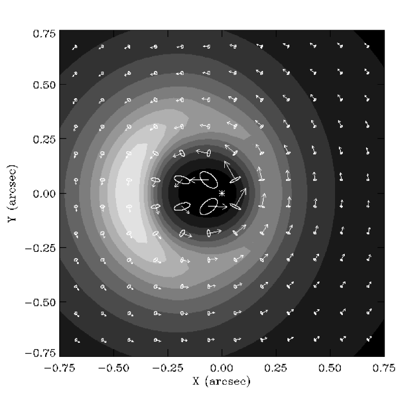
Figure 14: Disk-only mean velocity vectors (arrows) and velocity ellipsoids (ellipses) plotted over the surface density (contours) for Model 14 in Table 2, which has a Gaussian $F(e)$. Density contours are at 0.1, 0.2, …, 1.0 of the maximum density. An asterisk marks the location of the BH. Velocity ellipsoids in our disks are elongated in the radial direction, as expected from epicycle theory; most ellipsoids have a vertex deviations of $<10\hbox{${}^{\circ}$}$, and the maximum deviation is $\sim 30\hbox{${}^{\circ}$}$.

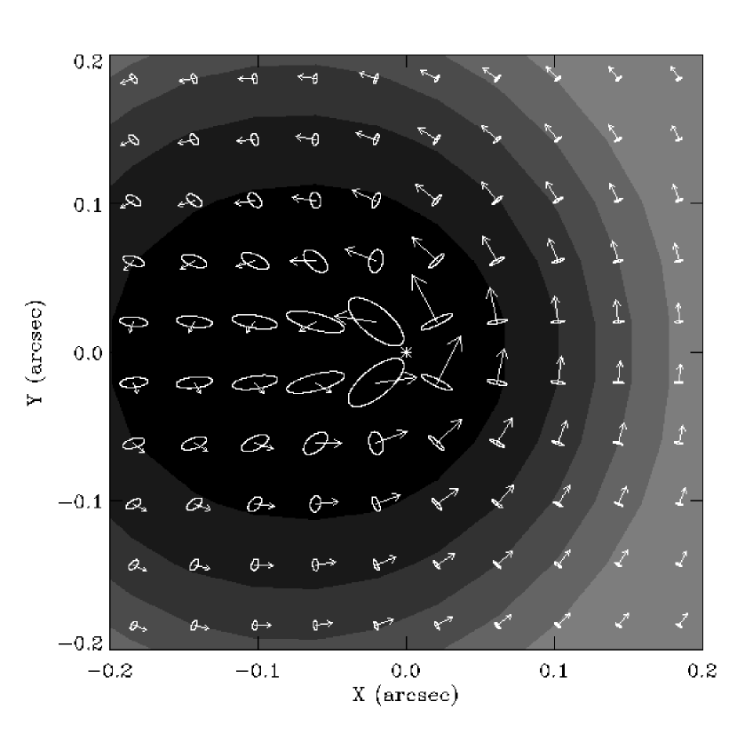
Figure 15: Same as in Figure 14 for the inner $0\hbox{$.\!\!^{\prime\prime}$}2$. Velocities are scaled to 1/5 of their values in Figure 14.

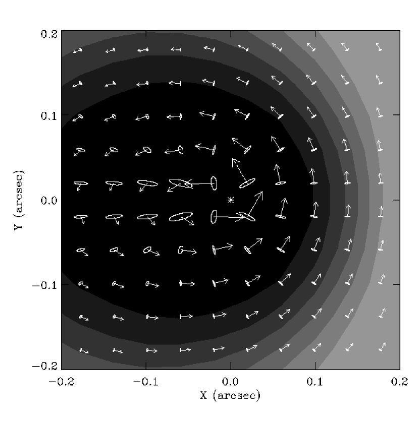
Figure 16: Similar to Figure 15, but for the disk in Model 13 in Table 2, which has a Rayleigh $F(e)$. Comparison with Figure 15 shows that the velocity dispersion in a disk with a Gaussian $F(e)$ is larger; the singularity at $e=0$ in the Gaussian distribution causes there to be an extra population of circular orbits, in addition to the normal eccentric population about $e_{0}(a)$.

Velocity ellipsoids are elongated in the radial direction, with vertex deviations typically less than $10\hbox{${}^{\circ}$}$ and always less than $30\hbox{${}^{\circ}$}$. From epicycle theory, $\sigma_{R}/\sigma_{T}\simeq 2$ for a Keplerian disk, where $\sigma_{R}$ and $\sigma_{T}$ are the radial and tangential dispersions, respectively (Binney & Tremaine 1987). Figure 17, which plots the ratio of major to minor axes for velocity ellipsoids as a function of radius, shows that ellipsoids from Models 14 (panel a) and 13 (panel b) approximately follow this trend beyond $r\sim 0\hbox{$.\!\!^{\prime\prime}$}4$. The point of transition away from Keplerian behavior occurs near the peak in $e_{0}(a)$ at $a\simeq 0\hbox{$.\!\!^{\prime\prime}$}3$.

Figure 17: Ratio of major to minor axes for disk-only velocity ellipsoids as a function of radius from the BH. (a) For Model 14, which has a Gaussian $F(e)$. (b) For Model 13, which has a Rayleigh $F(e)$. Dotted lines show an axis ratio of 2, which is expected from epicycle theory for a Keplerian disk. The departure from Keplerian behavior occurs near the peak in $e_{0}(a)$ at $a\simeq 0\hbox{$.\!\!^{\prime\prime}$}3$.

Comparison of Figures 15 and 16 shows that the disk velocity dispersion is larger in Model 14. This results from the singular nature of the Gaussian form of $F(e)$ at $e=0$ (see Section 2.2). The singularity causes there to be two orbit populations: first, a normal population of eccentric orbits around $e_{0}(a)$, and second, an extra population of circular orbits from the singularity. Differences in eccentricity between the two populations increases the velocity dispersion. The increase in dispersion is more prominent at radii where $e_{0}(a)$ is significantly different than zero.

5 Discussion

We find that the mass of the central BH in M31 is $5.62\pm 0.66\times 10^{7}\mbox{$\,M_{\odot}$}$. To put our result into context, we show BH mass estimates from various authors (see Section 4.2) in Figure 18 as a function of publication date. With the exception of the Dressler (1984) and KB99 values, all BH mass estimates are consistent with $M_{BH}\geq 5\times 10^{7}\mbox{$\,M_{\odot}$}$. Dressler’s value was estimated from gradients in $M/L$ and $\sigma$, rather than from kinematic and photometric modeling, and thus is only an order-of-magnitude estimate. KB99’s value was determined using the displacement of the UV peak relative to the bulge center, and may be low due to systematic errors in position measurements (PT03).

Figure 18: M31 BH mass versus publication date for the values reported in Section 4.2. Diamonds give the median value when a range of BH masses was published. Asterisks show BH masses for which no error estimate or range was provided. Also plotted is our best-fit value, $5.62\pm 0.66\times 10^{7}\mbox{$\,M_{\odot}$}$, denoted by a square, and the value computed from the $M_{BH}$ - $\sigma$ correlation given in Tremaine et al. (2002), $5.5\pm 1.5\times 10^{7}\mbox{$\,M_{\odot}$}$ (assuming their value of $160\pm 8\mbox{${\rm\,km\,s}^{-1}$}$ for the dispersion), denoted by a cross. The close agreement between our value and that from the correlation is remarkable.

The cross in Figure 18 shows the BH mass estimate from the slope of the $M_{BH}$ - $\sigma$ correlation given in Tremaine et al. (2002). Recall that the authors find $\log(M_{BH}/\mbox{$\,M_{\odot}$})=(8.13\pm 0.06)+(4.02\pm 0.32)\log(\sigma/200\mbox{${\rm\,km\,s}^{-1}$})$, from a sample of $31$ galaxies with reliable BH masses and dispersion measurements. For M31, $\sigma=160\pm 8\mbox{${\rm\,km\,s}^{-1}$}$ (Tremaine et al. 2002), which gives $M_{BH}=5.5\pm 1.5\times 10^{7}\mbox{$\,M_{\odot}$}$ using the correlation. The close agreement between this value and ours is rather remarkable.

Our BH mass is significantly lower than that found by PT03 in their fit to bulge-subtracted SIS/CFHT data (KB99) using Monte-Carlo simulations of eccentric disks built from non-interacting Kepler orbits. They find $M_{BH}=10.2\times 10^{7}\mbox{$\,M_{\odot}$}$ for their non-aligned model, in which the orientation of the disk is fitted to the data; error bars are not given with this measurement. This value is more than $60\%$ larger than the upper limit for our measurement.

Understanding this discrepancy is difficult, due to fundamental differences in model approximations. PT03 ignore disk self-gravity and precession, but include the three-dimensional structure of the disk; our disks include self-gravity and precession, but are assumed to be thin, and limited to two dimensions. PT03 suggest that ignoring the disk self-gravity is likely to cause the BH mass to be $10-20\%$ too large. However, it is unknown how including both self-gravity and precession together would further affect their mass value, especially if the precession rate is as large as we find in our models ($36.5\pm 4.2\mbox{$\rm\,km\,s^{-1}pc^{-1}$}$). Similarly, it is difficult to ascertain how including a vertical structure to our disks would affect $M_{BH}$, $\Omega$, and possibly other parameters.

Results from PT03 suggest that some vertical structure is needed to match the photometry. Their non-aligned model reproduces the well-defined double structure of M31’s nucleus, whereas our two-dimensional simulations produce crescent-shaped P1 structures. The dip in surface brightness between P1 and P2 is reproduced in their models, even with the disk at $i=54\hbox{${}^{\circ}$}$; our models possess overly-strong central surface brightness minima, unless a strong bulge cusp is included in the model. PT03 also give dynamical reasons for having vertical structure in the disk. Using results from studies of disk heating by two-body relaxation in protoplanetary disks (Ohtsuki, Stewart, & Ida 2002), they show that their non-aligned disk must have a vertical-to-radial axis ratio of $\sim 0.25$ in the radius range $0.5-1\hbox{${}^{\prime\prime}$}$. This being said, PT03 point out that the effect on the kinematics is less dramatic than for the photometry. Since weighting of the data is dominated by one and two-dimensional kinematics in our best fits (Table 2), our value for the BH mass should suffer only minor modulation with the addition of the third dimension. Vertical dispersion would increase the overall line of sight velocity dispersion, while minimally affecting the rotation curve; this would improve the fit in models like Model 2 ( Figure 5), which has a small dispersion spike.

PT03 present bulge-subtracted LOSVDs from unpublished STIS observations of M31’s nucleus (Bender et al. 2003) at a few locations within $\pm 0\hbox{$.\!\!^{\prime\prime}$}15$ of the UV peak, along with model LOSVDs extending another $\pm 0\hbox{$.\!\!^{\prime\prime}$}25$, in their Figure 15. We show corresponding LOSVDs for Models 14 and 13 as solid and dotted lines in Figure 19, respectively. LOSVDs from Bender et al. possess multiple maxima, some of which may be real features. Of particular interest are their LOSVDs at $0\hbox{$.\!\!^{\prime\prime}$}10$ and $0\hbox{$.\!\!^{\prime\prime}$}15$, both of which show a small bump near $v=750\mbox{${\rm\,km\,s}^{-1}$}$; our LOSVDs also show these bumps, which occur at supracircular velocities, as indicated by the arrows in our Figure 19. Supracircular peaks occur when the tangent point falls near the pericenters of orbits with substantial eccentricity. Such features arise from the density and eccentricity structure of the disk, and can be used as sensitive discriminants of disk structure in M31 (Salow & Statler 2001).

Figure 19: Disk-only LOSVDs near the UV peak for Model 14 (solid lines) and Model 13 (dotted lines) from Table 2, for the $0\hbox{$.\!\!^{\prime\prime}$}1$ wide STIS slit along PA$=39\hbox{${}^{\circ}$}$. The distance from the UV peak along the slit is given above each panel. Arrows mark the circular speed at the tangent point. These are to be compared with LOSVDs from unpublished STIS observations (Bender et al. 2003) presented in PT03 (their Figure 15). Both model and data show a small bump at supracircular velocities in the $0\hbox{$.\!\!^{\prime\prime}$}10$ and $0\hbox{$.\!\!^{\prime\prime}$}15$ Panels; these result from the density and eccentricity structure of the disk.

Model LOSVDs from PT03 do not have multiple maxima; instead, they find asymmetric LOSVDs with strong wings toward prograde velocities. However, their LOSVDs between $0\hbox{$.\!\!^{\prime\prime}$}10$ and $0\hbox{$.\!\!^{\prime\prime}$}20$ have a shoulder that appears to move inward toward $v=0\mbox{${\rm\,km\,s}^{-1}$}$ in the same manner as the bump at supracircular velocities does in our LOSVDs. This may be a signature of the tangent point traversing the pericenters of eccentric orbits, with the gap between the maxima somehow filled in by the density structure of the disk.

We show disk-only LOSVDs at the resolution of STIS along the kinematic axis (PA${}_{K}=56.4\hbox{${}^{\circ}$}$) in Figure 20 for Models 14, 12, and 10 from Table 2, which have BH masses of $5.55\times 10^{7}\mbox{$\,M_{\odot}$}$, $6.84\times 10^{7}\mbox{$\,M_{\odot}$}$, and $4.67\times 10^{7}\mbox{$\,M_{\odot}$}$, respectively. These are shown as predictions for upcoming STIS observations, which should yield $S/N\sim 120$ in the $4500-5500\AA$ region, and allow detailed features in the LOSVD to be seen (Cycle 12 ID-9859, E. Emsellem, PI). $M_{BH}$, $M_{d}$, and $\Omega$ all increase from Model 10 to Model 14 to Model 12. The most significant differences in LOSVDs are seen between Model 10 and the other two, mostly due to the $\sim 16\hbox{${}^{\circ}$}$ inclination difference. LOSVDs for Models 14 and 12 are similar throughout much of the near-UV peak region, though there are measurable differences in the number of maxima and their strength and location, especially between $-0\hbox{$.\!\!^{\prime\prime}$}10$ and $0\hbox{$.\!\!^{\prime\prime}$}05$. Thus, with high S/N, it should be possible to differentiate between models using LOSVDs.

Figure 20: Disk-only LOSVDs for Model 14 (solid lines), Model 12 (dotted lines), and Model 10 (dashed lines) from Table 2, for the $0\hbox{$.\!\!^{\prime\prime}$}1$ wide STIS slit along the kinematic axis (PA$=56.4\hbox{${}^{\circ}$}$). The distance from the UV peak along the slit is given above each panel. $M_{BH}$, $M_{d}$, and $\Omega$ all increase from Model 10 to Model 14 to Model 12; Model 10 is at $i=68\hbox{${}^{\circ}$}$, compared to $i=52.5\hbox{${}^{\circ}$}$ for the other two. These are shown as predictions for upcoming STIS observations at $S/N\sim 120$. The three models can be distinguished between $-0\hbox{$.\!\!^{\prime\prime}$}10$ and $0\hbox{$.\!\!^{\prime\prime}$}05$, so with high $S/N$ it should be possible to differentiate between models using LOSVDs.

The Bender et al. (2003) velocity dispersion profiles presented in PT03 (their Figure 12) deserve special mention. The dispersion spike in their bulge-subtracted STIS profile is offset from the UV peak by only $0\hbox{$.\!\!^{\prime\prime}$}08$, compared to the $\sim 0\hbox{$.\!\!^{\prime\prime}$}2$ offset found by B01 in both STIS (their Figure 11) and slit-averaged OASIS (their Figure 8) dispersion profiles. The large offset cannot be reproduced by our models. But the $\sim 0\hbox{$.\!\!^{\prime\prime}$}1$ discrepancy suggests that there may be a problem with the positional registration of the data in either the Bender et al. (2003) or B01 results. The Bender et al. results are bulge-subtracted, unlike in B01, but the addition of a bulge component should move the dispersion spike slightly closer to the UV peak, not away from it, if the BH is centered in the bulge. Bender et al.’s profile is favored by our models, which typically have the dispersion spike only slightly offset toward P2; for example, the dispersion profile for Model 10 (Figure 7) has a dispersion spike offset of $\sim 0.03$ from the UV peak.

If the dispersion spike really is offset from the UV peak by $\sim 0\hbox{$.\!\!^{\prime\prime}$}2$ toward P2, then either our models are essentially correct but missing a key ingredient, or the basic assumptions of the model incorrectly describe M31’s nucleus. This second possibility is unlikely, given that our models are able to reproduce many of the key features in both the kinematic and photometric data; the same holds true for models presented in T95, KB99, B01, Salow & Statler (2001), SS02, Jacobs & Sellwood (2001), and PT03. As for the first possibility, one suggestion is the addition of retrograde orbits. Our models include only prograde orbits. SS02, who build their model using an orbit library with both prograde and retrograde orbits, find that the fit near P2 is improved greatly with the addition of retrograde orbits comprising only $3.4\%$ of the total disk mass. However, the dispersion spike in their model is located very close to the UV peak, even with retrograde orbits (see their Figure 4). As a rough test, we added velocity moments from retrograde orbits comprising $0.05M_{d}$ to a few models before convolution with the PSF. A set of retrograde periodic orbits was found numerically in the same way as was done for the prograde orbits, and the moments were found using the DF, as in Section 2.3. We similarly found that the dispersion spike did not significantly move. It should be noted that these tests were performed using the same $F(a)$ and other disk parameters, excepting $M_{d}$, as the main eccentric disk itself, which may not realistically describe the hypothetical retrograde population.

Using a simple heuristic velocity model, B01 find that the best overall fit to FOC, STIS and slit-averaged OASIS kinematics requires a high velocity component in the central $0\hbox{$.\!\!^{\prime\prime}$}3$ aligned with the kinematic axis. This component is added to reproduce the abrupt jump in the FOC rotation curve near $x=0\hbox{$.\!\!^{\prime\prime}$}1$ (see Figure 5). B01 argue that, with the addition of this component, the dispersion spike is then just the result of the effect of velocity broadening. The high velocity component may be related to retrograde orbits. The question of whether or not retrograde orbits can affect the dispersion spike clearly needs further investigation.

We find that disks with $i=52.5\hbox{${}^{\circ}$}$ provide the best match to the two-dimensional kinematics and photometry. This inclination is consistent with that found by deprojecting the nucleus, assuming a thin disk (B01, SS02, P02), and with PT03’s fit for their non-aligned model. Thus, the nuclear disk is most likely not aligned with the large-scale disk of M31, which is at $i=77\hbox{${}^{\circ}$}$ with the line-of-nodes at PA${}_{n}=38\hbox{${}^{\circ}$}$ (T95). M31’s bulge is thought to be triaxial, and possibly aligned with the large-scale disk (Lindblad 1956, Stark 1977, Stark & Binney 1994, Berman 2001, Berman & Loinard 2002). The nuclear disk should then be subject to dynamical friction from the bulge, which acts to damp the inclination difference on the precession time ($\sim 10^{7}$ yr; PT03 and references therein). At that timescale, the inclination difference should have been damped out long ago, since absorption-index radial profiles suggest that the age of the nuclear disk is roughly $1/3$ that of the bulge (Sil’chenko et al. 1998), which is on order of a Hubble time. However, the recent photometric decomposition by P02 suggests that the inner bulge may be spherical, rather than triaxial. P02 finds that the overall bulge is fit best by two components; an inner, nearly spherical component (axis ratio $q=0.97\pm 0.02$) described by a Sérsic (1968) light profile with effective radius $3\hbox{$.\!\!^{\prime\prime}$}31$ and exponent $n=0.83$, and a large-scale, more elliptical component ($q=0.81\pm 0.01$) described by a Nuker law (Lauer et al. 1995) of break radius $66\hbox{$.\!\!^{\prime\prime}$}48$ and an asymptotic inner power law slope $\gamma=0.17$. The mass of the spherical component is $M_{s}=2.8\times 10^{7}\mbox{$\,M_{\odot}$}$, roughly half of the mass of the BH. If this is correct, then the bulge potential is spherical around the nucleus, which might allow the non-aligned orientation to survive, even if the outer bulge is triaxial. Another possible way to avoid dynamical friction from the bulge is to have an axisymmetric bulge which is aligned with the nuclear disk (PT03). It is intriguing that Ruiz (1976) finds that an axisymmetric bulge is consistent with kinematic and photometric data if $i=55\hbox{${}^{\circ}$}$.

All of the models presented in this paper have a backbone orbit sequence, $e_{0}(a)$, similar to that shown for Model 14 (the solid line in Figure 13c), in which there is no tendency for the orbits to switch their apoapses to the P2 side of the disk following the large negative eccentricity gradient. This is contrary to the the findings of S99 and Salow & Statler (2001). B01 and SS02 also find $e(a)$s similar to that for Model 14, though with a larger maximum eccentricity ($e_{max}\geq 0.6$). Many of our models do, however, show such a switch at low semimajor axis, before the maximum in $e_{0}(a)$ (see the dotted line in Figure 13c), as in Salow & Statler (2001). Tremaine (2001) finds such a switch on both sides of a maximum in $e(r)$, where $r$ is the radius from the central massive object, for certain slow $p$-modes in nearly Keplerian disks with softened gravity, using the WKB approximation (see his Figures 6 and 9); self-gravitating disks with significant velocity dispersion support prograde “pressure” modes, corresponding to Tremaine’s $p$-modes (B01). Models like ours can, in principle, possess $e_{0}(a)$s with an eccentricity sign switch after maximum, or on both sides of maximum, but only if $\Omega$ is decreased by about $40\%$ from the values we find in our fits to M31. For example, Figure 21a in Appendix A shows $e_{0}(a)$ for an arbitrary model with $\epsilon=0.2$ and $\Omega\simeq 12\mbox{$\rm\,km\,s^{-1}pc^{-1}$}$.

The small value for $e_{max}$ in our models ($0.21\pm 0.05$) is a consequence of the large precession rate ($36.5\pm 4.2\mbox{$\rm\,km\,s^{-1}pc^{-1}$}$). Lagrange’s planetary equations for the secular evolution orbital elements undergoing an external perturbation have $\Omega\simeq(1/na^{2}e)(\partial R/\partial e)$, where $n$ is the mean motion and $R$ is the Disturbing Function, or perturbing potential (Murray & Dermott 1999); thus, $e\sim 1/\Omega$. Models in B01 and SS02 have larger values for $e_{max}$ ($\sim 0.7$) and lower precession rates ($3\mbox{$\rm\,km\,s^{-1}pc^{-1}$}$ and $16\mbox{$\rm\,km\,s^{-1}pc^{-1}$}$, respectively), in agreement with the rough trend $e_{max}\sim 1/\Omega$. It is interesting to note that the precession rate measured using the Tremaine & Weinberg (1984) method gives $\Omega=34\pm 8\mbox{$\rm\,km\,s^{-1}pc^{-1}$}$ and $\Omega=20\pm 12\mbox{$\rm\,km\,s^{-1}pc^{-1}$}$ for a Nuker and Sérsic fit to the bulge (Sambhus & Sridhar 2000), respectively, both of which are consistent with our value for $\Omega$.

The question of how the eccentric disk formed in M31 is still an open question. Currently, two formation scenarios are favored: first, that an initially axisymmetric disk becomes lopsided due to an external perturbation (T95, B01, P02, PT03), or by a dynamical instability (Touma 2002, SS02); second, that the disk is formed when an infalling star cluster is tidally stripped by the central BH (Bekki 2000, Quillen & Hubbard 2003). The external perturbation may come from a globular cluster or giant molecular cloud passing by the disk (B01, P02), or by the influence of dynamical friction from the bulge (T95, PT03), both of which may excite the mean eccentricity of the disk. Using a softened analogue of the Laplace-Lagrange secular theory for interacting planar Keplerian rings, Touma (2002) showed that a small fraction of counter-rotating stars is sufficient to cause a pre-existing disk to develop a linear $m=1$ instability. The retrograde orbits may have originated from a tidally disrupted stellar cluster on a retrograde orbit (SS02); Tremaine et al. (1975) have shown that dynamical friction can cause globular clusters to spiral into the nucleus and be tidally disrupted.

Bekki (2000) performed N-body simulations in which a globular cluster is disrupted by a massive BH, and found that a long-lived eccentric disk can be produced. The progenitor cluster, however, was only about one-tenth as massive as the disk in M31. From simple tidal disruption arguments in a single disruption-event scenario, Quillen & Hubbard (2003) show that many Galactic globular clusters satisfy core radius and density requirements necessary for the formation of an eccentric disk near the BH, supporting Bekki’s simulations. Normal globular clusters are not massive enough, however, to be plausible progenitors, and their colors are unlike those in the nucleus. Instead, Quillen & Hubbard suggest that a dense bulge core or nuclear star cluster might be the progenitor, since both can be massive and compact enough to satisfy requirements for M31. They point out that if merging galaxy bulges can form eccentric disks, then such disks would be a natural consequence of hierarchical galaxy formation.

An interesting connection may exist between the disruption-event scenario and the spherical inner bulge found by P02. Milosavljevic & Merritt (2001) perform N-body simulations of merging stellar systems with black holes, and find that the inward-spiraling binary black holes scatter stars from the center via gravitational slingshot. P02 suggests that these ejected stars could form a spherical distribution after redistribution in phase space. If this is true, then the presence of the spherical bulge component would lend support to the idea that the disk formed during a merger of galaxies with central BHs.

6 Conclusion

Our models of eccentric stellar disks around central black holes incorporate self-gravity, finite velocity dispersion, and gravity-induced precession, in a self-consistent way. We have used these models to perform the first detailed fit to the nucleus of M31 which includes both one and two-dimensional kinematics and photometry; the data set includes FOC, STIS, and SIS one-dimensional kinematics, OASIS two-dimensional kinematics, and one and two-dimensional WFPC2 photometry. The primary result of this modeling effort is an accurate measurement of the mass of the central black hole in M31. We find that $M_{BH}=5.62\pm 0.66\times 10^{7}\mbox{$\,M_{\odot}$}$. This value is consistent with the $M_{BH}-\sigma$ correlation (Tremaine et al. 2002), which gives a value of $5.5\pm 1.5\times 10^{7}\mbox{$\,M_{\odot}$}$.

We find eccentric disks with large precession rates ($\Omega=36.5\pm 4.2\mbox{$\rm\,km\,s^{-1}pc^{-1}$}$) and small maximum eccentricities ($e_{max}=0.21\pm 0.05$) for the backbone orbit sequence, $e_{0}(a)$. The backbone orbits possess a characteristic non-monotonic distribution with a steep negative eccentricity gradient ($de/da<0$) through the densest part of the disk, which gives rise to distinctive multi-modal LOSVDs for lines of sight near the central BH. Such features may be used to further constrain model parameters when LOSVDs from upcoming high S/N STIS observations of M31’s nucleus become available.

Although our models provide an accurate estimate for the BH mass, there is room for improvement. We have assumed that the disk in M31 is thin. The disk may have non-negligible vertical structure, however, which could slightly alter our BH estimate. Vertical velocity dispersion can be added to our models by including dispersions in inclination, $i$, and in the longitude of the ascending node, $\Omega_{n}$, in our prescription for populating quasi-periodic orbits about the backbone orbit sequence. We would then have a DF which includes all five integrals of motion in the three-dimensional Kepler problem; that is, $f(a,e,\omega,i,\Omega_{n})$; PT03 demonstrate how the third dimension can be included in this way. Further improvement may require that new bulge models be considered, to better fit the behavior of the models within the central $0\hbox{$.\!\!^{\prime\prime}$}4$ of the nucleus. More flexible versions of $F(a)$ and a population of retrograde orbits can also help in this regard. Retrograde orbits should be included self-consistently with their own DF and parameters, to determine if the location of the dispersion spike can be adjusted by their presence.

The eccentric disk picture for the nucleus of M31 is clearly the correct one, given the success that our models, along with those of other investigators, have at reproducing most of the asymmetric features in the kinematic and photometric data. A complete description of the available data should be possible with models like ours, which already include most of the key physical ingredients, once they are extended as mentioned above. Such models should be flexible enough to probe the connection between the BH and nuclear stars in greater detail, and may yield new clues about the formation of eccentric disks around BHs. With the knowledge gained from detailed study of these models, other systems exhibiting features like those seen in M31, which do not have resolved Keplerian-dominated regions ($r_{k}$), can be investigated with confidence, as long as the sphere of influence of the BH ($r_{h}$) is resolved.

Galaxies with central properties similar to those in M31 are already known to exist. NGC 4486B, a low-luminosity E1 companion of M87, is already known to possess two brightness peaks (Lauer et al. 1996). This galaxy has no distinct nucleus, however, and its P1-P2 separation is $\sim 10$ - $13$ pc ($\sim 0\hbox{$.\!\!^{\prime\prime}$}15$ at $D=16$ Mpc), which is about six times that in M31; also, its P1 and P2 have nearly the same brightess, unlike in M31. Models like ours may be applicable, with some modification to the density structure to account for lack of a distinct nucleus. Dynamical modeling of spectroscopic data from SIS/CFHT suggests that NGC 4486B harbors a BH of mass $\sim 6\times 10^{8}\mbox{$\,M_{\odot}$}$ (Kormendy et al. 1997). Kormendy et al. find $\sigma\simeq 130\mbox{${\rm\,km\,s}^{-1}$}$, which, along with the aforementioned BH mass, implies that $r_{h}\simeq 2\hbox{${}^{\prime\prime}$}$ (probably as an upper limit), which can be resolved by STIS/HST. Further examples are shown by Lauer et al. (2002), who recently discovered six early-type galaxies with surface brightness profiles that decrease inward near their centers, reminiscent of the central dip in surface brightness found in M31. These galaxies harbor torus-like brightness distributions, rather than double nuclei. Such structures can possibly be fit by a thin disk with low $\epsilon/\Omega$, which is only slightly asymmetric. The sharpest structure observed in the sample is in the S0 galaxy NGC 3706, which has a bright stellar torus of radius $r\sim 20$ pc ($0\hbox{$.\!\!^{\prime\prime}$}12$ at $D=35$ Mpc). Using the velocity dispersion observations from Carollo & Danziger (1994), the $M_{BH}$ - $\sigma$ correlation gives $M_{BH}\simeq 6\times 10^{8}\mbox{$\,M_{\odot}$}$ for this galaxy. With this mass, $r_{h}\simeq 0\hbox{$.\!\!^{\prime\prime}$}15$. Modeling this galaxy will require observations with higher resolution than is currently available, but which may be available in the near future.

Appendix A Extending the Orbit Sequence

Beyond the 2:1 resonance it becomes difficult to find nearly-elliptical periodic orbits using the method described in Section 2.3. Periodic orbits beyond this resonance belong to various resonant families. Since the 2:1 resonance falls within $R_{d}$ for models with larger values of $\Omega$, we must approximate the backbone structure of the disk in those cases. When truncation occurs, we simply assume that the sequence of nearly-Keplerian orbits continues out to $R_{d}$. We do this in a way that mimics the behavior of $e_{0}(a)$ for those models whose orbit sequence does not truncate, using the decaying oscillatory function

$$E(a)=\exp\left(-Aa^{2}\right)\cos\left(Ba+C\right).$$ (A1)

We fit this function to the last $10$ orbits in $e_{0}(a)$, just before the cutoff. Figure 21 shows three examples of extended $e_{0}(a)$ functions for arbitrary models. The disk structure and dynamics was found to be insensitive to the choice of the extending function for a wide range of decaying functions.

Figure 21: Three examples of extended $e_{0}(a)$ functions, using $E(a)$ in Equation A1. The dotted lines show the point where the orbit sequence truncates, near the 2:1 resonance. The three models shown are not from the grid of 24 best-fit models; they are arbitrary models showing three different types of behavior typically found for $e_{0}(a)$ in the M31-like region of parameter space.

References

- (1) Bacon, R., Emsellem, E., Monnet, G., & Nieto, J. L. 1994, A&A, 281, 691
- (2) Bacon, R., Emsellem, E., Combes, F., Copin, Y., Monnet, G., & Martin, P. 2001, A&A, 371, 409 (B01)
- (3) Bekki, K. 2000, ApJ, 540, L79
- (4) Bender, R., Kormendy, J., Bower, G., Green, R., Gull, T., Hutchings, J. B., Joseph, C. L., Kaiser, M. E., Nelson, C. H., & Weistrop, D. 2003, in preparation
- (5) Berman, S. 2001, A&A, 371, 476
- (6) Berman, S., & Loinard, L. 2002, MNRAS, 336, 477
- (7) Binney, J., & Tremaine, S. 1987, Galactic Dynamics (Princeton: Princeton Univ. Press)
- (8) Bower, G. A., et al. 1998, ApJ, 492, L111
- (9) Brown, T. M., Ferguson, H. C., Stanford, S. A., & Deharveng, J. 1998, ApJ, 504, 113
- (10) Carollo, C. M. & Danziger, I. J. 1994, MNRAS, 270, 523
- (11) Chokshi, A. & Turner, E. L. 1992, MNRAS, 259, 421
- (12) Corbin, M. R., O’Neil, E., & Rieke, M. J. 2001, AJ, 121, 2549
- (13) Davidge, T. J., Rigaut, F., Doyon, R., & Crampton, D. 1997, AJ, 113, 2094
- (14) Dones, L. & Tremaine, S. 1993, Icarus, 103, 67
- (15) Dressler, A. 1984, ApJ, 286, 97
- (16) Dressler, A., & Richstone, D. O. 1988, ApJ, 324, 701
- (17) Eckart, A. & Genzel, R. 1996, Nature, 383, 415
- (18) Emsellem, E., & Combes, F. 1997, A&A, 323, 674
- (19) Ferrarese, L. & Merritt, D. 2000, ApJ, 539, L9
- (20) Freedman, W. L. & Madore, B. F. 1990, ApJ, 365, 186
- (21) Gebhardt, K. et al. 2000a, ApJ, 539, L13
- (22) Gebhardt, K. et al. 2000b, ApJ, 543, L5
- (23) Gebhardt, K., et al. 2001, AJ, 122, 2469
- (24) Gebhardt, K., et al. 2003, ApJ, 583, 92
- (25) Ghez, A. M., et al. 1998, ApJ, 509, 678
- (26) Ghez, A. M., et al. 2003, ApJ, 586, L127
- (27) Haehnelt, M. G. & Rees, M. J. 1993, MNRAS, 263, 168
- (28) Hagiwara, Y. et al. 2003, MNRAS, 344, L53
- (29) Harms, R. J. et al. 1994, ApJ, 435, L35
- (30) Ho, L. C., Filippenko, A. V., & Sargent, W. L. W. 1997, ApJ, 487, 568
- (31) Holland, S. 1998, AJ, 115, 1916
- (32) Ishihara, Y. et al. 2001, PASJ, 53, 215
- (33) Jacobs, V., and Sellwood, J. A. 2001, ApJ, 555, L25
- (34) Jalali, M. A. & Rafiee, A. R. 2001, MNRAS, 320, 379
- (35) Kennicutt, R. C., et al. 1998, ApJ, 498, 181
- (36) King, I. R., Stanford, S. A., & Crane, P. 1995, AJ, 109, 164 (K95)
- (37) Kormendy, J. 1988, ApJ, 325, 128
- (38) Kormendy, J. 1993, in IAU Symp. 153, Galactic Bulges, ed. H. Dejonghe & H. J. Habing (Dordrecht:Kluwer), 209
- (39) Kormendy, J., & Richstone, D. 1995, ARA&A, 33, 581
- (40) Kormendy, J., et al. 1997, ApJ, 482, L139
- (41) Kormendy, J. & Bender, R. 1999, ApJ, 522, 772 (KB99)
- (42) Krist, J., & Hook, R. 1999, The Tiny Tim User’s Guide (Baltimore: STScI)
- (43) Lauer, T. R., et al. 1993, AJ, 106, 1436 (L93)
- (44) Lauer, T. R., et al. 1995, AJ, 110, 2622
- (45) Lauer, T. R., et al. 1996, ApJ, 471, L79
- (46) Lauer, T. R., Faber, S. M., Ajhar, E. A., Grillmair, C. J., & Scowen, P. A. 1998, AJ, 116, 2263 (L98)
- (47) Lauer, T. R., et al. 2002, AJ, 124, 1975
- (48) Light, E. S., Danielson, R. E., & Schwarzschild, M. 1974, ApJ, 194, 257
- (49) Lindblad, B. 1956, Stockholms Obs. Ann., 19, No. 2
- (50) Lynden-Bell, D. 1969, Nature, 223, 690
- (51) Macchetto, F., et al. 1997, ApJ, 489, 579
- (52) Magorrian, J. et al. 1998, AJ, 115, 2285
- (53) Marconi, A. et al. 2003, ApJ, 586, 868
- (54) Merritt, D. et al. 2001, Science, 293, 1116
- (55) Milosavljević, M. & Merritt, D., 2001, ApJ, 563, 34
- (56) Miyoshi, M. et al. 1995, Nature, 373, 127
- (57) Mould, J. et al. 1989, ApJ, 339, L21
- (58) Murray, C. D. & Dermott, S. F. 1999, Solar System Dynamics (Cambridge: Cambridge Univ. Press)
- (59) Nieto, J.-L. et al. 1986, A&A, 165, 190
- (60) Ohtsuki, K., Stewart, G. R., & Ida, S. 2002, Icarus, 155, 436
- (61) Peiris, H. V. & Tremaine, S. 2003, ApJ, in press (astro-ph/0307412) (PT03)
- (62) Peng, C. Y. 2002, AJ, 124, 294 (P02)
- (63) Peterson, B. M. & Wandel, A. 1999, ApJ, 521, L95
- (64) Peterson, B. M. & Wandel, A. 2000, ApJ, 540, L13
- (65) Press, W. H., Teukolsky, S. A., Vetterling, W. T., & Flannery, B. P. 1992, Numerical Recipes in Fortran, 2nd ed. (Cambridge: Cambridge Univ. Press)
- (66) Quillen, A. C. & Hubbard, A. 2003, AJ, 125, 2998
- (67) Rees, M. J. 1984, Ann. Rev. Astron. Astrophys., 22, 471
- (68) Richstone, D., Bower, G., & Dressler, A. 1990, ApJ, 353, 118
- (69) Ruiz, M. T. 1976, ApJ, 207, 382
- (70) Salow, R. M., & Statler, T. S. 2001, ApJ, 551, L49
- (71) Sambhus, N., & Sridhar, S. 2000, ApJ, 539, L17
- (72) Sambhus, N., & Sridhar, S. 2002, A&A, 388, 766 (SS02)
- (73) Schödel, T., et al. 2002, Nature, 419, 694
- (74) Schwarzschild, M. 1979, ApJ, 232, 236
- (75) Sérsic, J. L. 1968, Atlas de Galaxias Australes (Córdoba: Obs. Astron. Univ. Córdoba)
- (76) Sil’chenko, O. K., Burenkov, A. N., & Vlasyuk, V. V. 1998, A&A, 337, 349
- (77) Soltan, A. 1982, MNRAS, 200, 115
- (78) Sridhar, S., and Touma, J. 1999, MNRAS, 303, 483
- (79) Stanek, K. Z. & Garnavich, P. M. 1998, ApJ, 503, L131
- (80) Stark, A. A. 1977, ApJ, 213, 368
- (81) Stark, A. A., & Binney, J. 1994, ApJ, 426, L31
- (82) Statler, T. S. 1999, ApJ, 524, L87 (S99)
- (83) Statler, T. S., King, I. R., Crane, P., & Jedrzejewski, R. I. 1999, AJ, 117, 894
- (84) Statler, T. S. & Salow, R. M. 2000, BAAS, 32, 865
- (85) Touma, J. R. 2002, MNRAS, 333, 583
- (86) Tremaine, S., Ostriker, J. P., & Spitzer, L. 1975, ApJ, 196, 407
- (87) Tremaine, S. & Weinberg, M. D. 1984, ApJ, 282, L5
- (88) Tremaine, S. 1995, AJ, 110, 628 (T95)
- (89) Tremaine, S. 2001, AJ, 121, 1776
- (90) Tremaine, S., et al., 1994, AJ, 107, 634
- (91) Tremaine, S., et al., 2002, ApJ, 574, 740
- (92) van der Marel, R. P. et al. 1994, MNRAS, 268, 521
- (93) van der Marel, R. P., & van den Bosch, F. C. 1998, AJ, 116, 2220
- (94) Verolme, E. K. et al. 2002, MNRAS, 335, 517
- (95) Vestergaard, M. 2002, ApJ, 571, 733