CMBfit: Rapid WMAP likelihood calculations with normal parameters

Abstract

We present a method for ultra-fast confrontation of the WMAP cosmic microwave background observations with theoretical models, implemented as a publicly available software package called CMBfit, useful for anyone wishing to measure cosmological parameters by combining WMAP with other observations. The method takes advantage of the underlying physics by transforming into a set of parameters where the WMAP likelihood surface is accurately fit by the exponential of a quartic or sextic polynomial. Building on previous physics based approximations by Hu et al., Kosowsky et al. and Chu et al., it combines their speed with precision cosmology grade accuracy. A Fortran code for computing the WMAP likelihood for a given set of parameters is provided, pre-calibrated against CMBfast, accurate to $\Delta\ln{\cal L}\sim 0.05$ over the entire $2\sigma$ region of the parameter space for 6 parameter “vanilla” $\Lambda CDM$ models. We also provide 7-parameter fits including spatial curvature, gravitational waves and a running spectral index.

I Introduction

The impressive sensitivity of the long awaited Wilkinson Microwave Anisotropy Probe (WMAP) data allows for unprecedented constraints on cosmological models [1, 2, 3, 4, 5, 6]. The measurements have strengthened the case for the cosmological concordance model[6], the inflationary $\Lambda$CDM model, a flat Universe which is currently accelerating due to mysterious dark energy, where most matter is in the form of collisionless cold dark matter, and where the initial conditions for the fluctuations are adiabatic. Because of well known cosmic microwave background (CMB) parameter degeneracies [18, 5, 11], the true impressiveness of the data is most clearly demonstrated by either imposing reasonable priors, combining the data with complimentary data sets, or both. The most recent precision data-sets are the Sloan Digital Sky Survey (SDSS) galaxy power spectrum (SDSS) [7] and a new Supernovae Ia compilation [10], and combining these with the WMAP constraints have further narrowed error bars [8], giving us cosmological parameters at a precision not thought possible only few years ago.

So how are CMB data-sets used to estimate parameters? Although constraints on cosmological parameters from the CMB can in principle be extracted directly from the maps themselves, this is effectively prohibited by the huge computational power necessary to perform the required likelihood calculations (although for a novel approach, see [15]). Instead, the more efficient parameter estimation method commonly employed uses the angular power spectrum of the map as an intermediate step[12, 13, 14].

Likelihoods on the basis of power spectrum constraints are much faster to calculate, the slowest step being the computation of the angular power spectrum numerically. This can be done either through integration of the full Boltzmann equation (with CMBfast [22] or the modifications CAMB[24] or CMBEASY[28]) or using an approximate shortcut such as DASh[27]. Although steady improvements in both computer power and algorithm performance have made these calculations significantly faster, the CMB power spectrum likelihood calculation is still the bottleneck in any parameter estimation process by many orders of magnitude.

Another problem with the estimation process are the near-degeneracies between some cosmological parameters. Elongated, banana shaped contours on the likelihood surface make search algorithms less efficient. Several authors have advocated various transformations from cosmological parameters to “physical” parameters more directly linked to features in the power spectrum[18, 20]. Chu et al. [21] advocated a new such set of “normal” parameters whose probability distributions are well fitted by Gaussian distributions.

Our key idea explored in this paper is that if the likelihood function is roughly a multivariate Gaussian in the transformed parameters, then it should be very accurately approximated by the exponential of a convenient higher-order polynomial. A Gaussian likelihood surface ${\cal L}$ corresponds to the log-likelihood $\ln{\cal L}$ being quadratic, and a quadratic Taylor expansion is of course an accurate approximation of any function near its maximum. Very far from the maximum, the Gaussian approximation again becomes accurate, since both it and the true likelihood ${\cal L}$ are vanishingly small. We will see that in most cases, small cubic and quartic corrections to $\ln{\cal L}$ help provide a near-perfect fit to ${\cal L}$ everywhere. The WMAP team employed such quartic fits to determine reasonable step sizes for their Markov Chain Monte Carlo search algorithm [6]. Here we go further and show how polynomial fits can conveniently store essentially all the cosmological information inherent in the WMAP power spectra. This reduces calculation of CMB likelihoods to simply evaluating the exponential of an $n^{th}$ order polynomial. Although CMBfast still needs to be run in order to obtain a sufficient sampling of the likelihood surface, this only has to be done once for each model space and dataset. For the models explored in this paper, it has already been done and the polynomial coefficients have been obtained. The polynomial fit can thus be used to run Monte Carlo Markov Chains (MCMC) including various non-CMB data-sets many orders of magnitude faster, dramatically reducing the need for computing power for cosmological parameter estimation purposes involving WMAP data. This is an improvement on importance sampling methods which notoriously depletes the chain of points as the added data sets shift or narrow the confidence regions. It means joint likelihood analyses between WMAP and other surveys which would previously take weeks or months of computer time on a good workstation being finished in an afternoon.

As mentioned, the last few years have seen the rise of a cosmological concordance model[25, 5, 8], the $\Lambda$CDM flat inflationary cosmology which has been confirmed and strengthened by WMAP, SDSS and new supernova observations. However as cosmological ideas and trends change, we choose to keep an open mind and allow for extensions to the 6-parameter inflationary $\Lambda$CDM model by including models with spatial curvature, gravitational waves and a running scalar spectral index. To allow the user to include CMB polarization information separately, we also perform separate likelihood fits excluding and including WMAP polarization data for the 6 parameter scenario.

II Method

Our approach in this paper consists of three steps:

1. Acquire a sample of the likelihood surface as a function of cosmological parameters. This is done through a Markov Chain Monte Carlo sampling of parameter space.

2. Transform from cosmological parameter space into normal parameters. This will make the likelihood surface close to Gaussian in these parameters, thereby increasing significantly the accuracy of the polynomial fit.

3. Fit of the log-likelihood surface to an $n^{th}$ order polynomial. The polynomial degree $n$ is optimized to the the likelihood-surface sampling density using a training set/test set approach.

Below we describe each of the above steps in detail.

A The Cosmological Parameters

We follow standard work[5, 25] in the field and parameterize our cosmological model with the $13$ parameters

$${\mathbf{p}}=\left(\tau,\Omega_{k},\Omega_{\Lambda},w,\omega_{d},\omega_{b},f_{\nu},A_{s},n_{s},\alpha,r,n_{t},b\right)$$ (1)

These parameters are the reionization optical depth, $\tau$, curvature energy density $\Omega_{k}$, the dark energy density $\Omega_{\Lambda}$, the dark energy equation of state $w$, the physical dark matter and baryon densities $\omega_{d}\equiv\Omega_{d}h^{2}$ and $\omega_{b}\equiv\Omega_{b}h^{2}$, the fraction of dark matter that is warm (massive neutrinos) $f_{\nu}$, the primordial amplitudes and tilts of the scalar and tensor fluctuations respectively $A_{s},n_{s},A_{t},n_{t}$ and the running of the scalar tilt $\alpha$. Here $A_{s},n_{s}$ and $\alpha$ are defined by the Ansatz $P_{*}(k)=A_{s}(k/k_{eval})^{n_{s}+\alpha\ln k}$, and similarly for the tensor case. $b$ is the galaxy bias $b^{2}=P_{galaxy}(k)/P(k)$. For a comprehensive cosmological parameter summary, see Table 1 of [8].

As stated in the introduction, we base our work around the adiabatic $\Lambda$CDM cosmological model, $\{\tau,\Omega_{\Lambda},\omega_{d},\omega_{b},n_{s},A_{s}\}$, a 6-parameter subspace of the 13 parameters. This is close to the minimal number of free parameters needed explain the data (the one exception being $n_{s}$, which is still consistent with unity) and assumes a pure cosmological constant and negligible spatial curvature, tensor fluctuations, running tilt, warm dark matter or hot dark matter As [5, 8], we also consider models with added “spice” such as curvature, tensor contributions and running tilt. We confine ourselves to a maximum of 7 parameters per model, i.e., to models with $\Lambda$CDM + a 7^th free parameter.

B The Likelihood

The fundamental quantity that one wants to estimate is the probability distribution function (PDF) of the parameters vector ${\bf p}$, $P({\bf p}|{\bf d})$, given the data, ${\bf d}$, and whatever prior assumptions and knowledge we may have about the parameters. The quantity we directly evaluate, however, is the probability of measuring the data given the parameters, $P({\bf d}|{\bf p})$ through a goodness-of-fit test. It is this distribution, when thought of as a function of the parameters, that we refer to as the likelihood, ${\cal L}({\bf p})\equiv P({\bf d}|{\bf p})$. The probability distribution function for the parameters is then related to the likelihood through Bayes’ theorem:

$$P({\bf p}|{\bf d})\propto P({\bf d}|{\bf p})P_{prior}({\bf p})$$ (2)

where $P_{prior}$ is the prior probability distribution of the parameters.

For ideal, full-sky, noiseless experiments, exact likelihood calculation is simple and fast. However, due to foreground contamination (the Galaxy, point sources etc.), only a fraction of the sky can be used for analysis. This leads to correlations between different multipoles and it becomes computationally prohibitive to calculate the exact likelihood function. Consequently, various approximations exist on which much work has been focused[6, 16] (for an excellent review of CMB likelihood calculations see [17]). In all our WMAP likelihood calculations we employ the latest version of the likelihood approximation routines supplied by the WMAP team. These routines take all effects into account, use an optimal combination of the various approximations, and are well tested through simulations[6]. As input, they take the CMB power spectrum, which we compute with CMBfast.

C Fitting to an $n^{th}$ order polynomial

Let us now look at how the polynomial fit is performed in detail. We start with a sample of N points ${\bf p}_{1},...,{\bf p}_{N}$ in the $d$-dimensional parameter space where the likelihood ${\cal L}({\bf p})$ has been evaluated, and wish to fit $\ln{\cal L}({\bf p})$ to a polynomial. Let $\langle{\bf p}\rangle$ denote the average of the parameter vectors ${\bf p}_{i}$ in our sample and let ${\bf C}\equiv\langle{\bf p}{\bf p}^{t}\rangle-\langle{\bf p}\rangle\langle{\bf p}\rangle^{t}$ denote the corresponding covariance matrix. To improve the numerical stability of our fitting, we work with transformed parameters that have zero mean and unit covariance matrix:

$${\bf z}\equiv{\bf E}({\bf p}-\langle{\bf p}\rangle),$$ (3)

where ${\bf E}$ is a matrix satisfying ${\bf E}{\bf C}{\bf E}^{t}={\bf I}$ so that $\langle{\bf z}{\bf z}^{t}\rangle={\bf E}\langle({\bf p}-\langle{\bf p}\rangle)({\bf p}-\langle{\bf p}\rangle)^{t}\rangle{\bf E}^{t}={\bf I}$, the identity matrix. There are many such choices of ${\bf E}$ — we make the choice where the rows of ${\bf E}$ are the eigenvectors the parameter covariance matrix ${\bf C}$ divided by the corresponding eigenvalues, so our transformed parameters ${\bf z}$ can be interpreted as simply uncorrelated eigenparameters rescaled so that they all vary on the same scale (with unit variance). This transformation turns out to be crucial, changing the matrix-inversion below from quite ill-conditioned to numerically well-conditioned.

A $n^{th}$ order polynomial in these $d$ transformed parameters has $M={n+d\choose n}={(n+d)!\over n!d!}$ terms:

$$y\equiv\log{{\cal L}} = q_{0}+\sum_{i}q^{i}_{1}z_{i}+\sum_{i_{1}\leq i_{2}}q_{2}^{i_{1}i_{2}}z_{i_{1}}z_{i_{2}}+$$ (5)

$$+\sum_{i_{1}\leq i_{2}\leq\cdots\leq i_{d}}q_{n}^{i_{1}i_{2}\cdots i_{d}}z_{i_{1}}z_{i_{2}}\cdots z_{i_{d}}$$

We assemble all necessary products of $z_{i}$’s into an $M$-dimensional vector

$${\bf x}=\{1,z_{1},\cdots,z_{d},z_{1}z_{1},\cdots,\Pi_{i=1,n}z_{i}\},$$ (6)

and the corresponding coefficients $q$ into another $M$-dimensional vector

$${\bf q}=\{q_{0},q_{1}^{1},\cdots,q_{1}^{d},q_{1}^{11},\cdots,q_{n}^{d...d},\cdots\},$$ (7)

which simplifies eq. (5) to

$$y={\bf x}\cdot{\bf q}.$$ (8)

We now assemble the $N$ measured log-likelihoods $y_{i}$ from our Monte Carlo Markov Chain into an $N$-dimensional vector ${\bf y}$ and the corresponding ${\bf x}$-vectors into an $N\times M$-dimensional matrix ${\bf X}$, so the $N$-dimensional vector of residual errors $\mathbf{\varepsilon}$ from our polynominal fit is

$$\mathbf{\varepsilon}\equiv{\bf y}-{\bf X}{\bf q}.$$ (9)

We choose the fit that minimizes the rms residual. i.e., that minimizes $|\mathbf{\varepsilon}|^{2}$. Differentiating with respect to ${\bf q}$ gives the standard least-squares result

$${\bf q}=\left({\bf X}^{t}{\bf X}\right)^{-1}{\bf X}^{t}{\bf y}.$$ (10)

Thus the minimizing the sum of squares in the end comes down to the inversion of an $M\times M$ matrix. The size of the matrix, $M=(n+d)!/n!d!$, depends on both number of parameters and the polynomial degree, ranging from $M=210$ for a 6 parameter 4th order fit to $M=1716$ for a 7 parameter 6th order fit (see table I for the number of coefficients for various relevant cases).

Parameters	$n=2$	$n=3$	$n=4$	$n=5$	$n=6$
5	21	56	126	252	462
6	28	84	210	462	924
7	36	120	330	792	1716
8	45	165	495	1287	3003
9	55	220	715	2002	5005
10	66	286	1001	3003	8008
11	78	364	1365	4368	12376

TABLE I.: Number of coefficients for a model with $d$ parameters fitting to an $n^{th}$ order polynomial. The number of coefficients range from 28 for a 6 parameter $2^{nd}$ order fit to a whopping 12376 for an 11 dimensional model and $6^{th}$ order polynomial.

Chu et.al.[21] have illuminated the problems of fitting a Gaussian directly to the 6- (or higher) dimensional likelihood surfaces and have argued that the surfaces may be too sparsely sampled in these dimensions. Consequently [21] fits to the 2D marginalized distributions and reconstructs the 6D likelihood function from this. Our interpretation is that the difficulties with fitting a quadratic polynomial to the 6 or 7 dimensional log-likelihood surface shows that the likelihood surface deviates too much from a Gaussian and that a higher order polynomial is required to reproduce the likelihood to sufficient accuracy. This interpretation is shared by [6] who use a $4^{th}$ order polynomial to calculate MCMC step sizes.

It is an advantage of our approach that we do not rely strictly on the chain we fit to being a fair statistical sample of the likelihood. Indeed we only need the value of the likelihood at a sufficient number of points, and we are as such insensitive to statistical errors such as sampling errors and poor mixing. The way that the input points ${\bf p}_{i}$ sample parameter space tells the fitting algorithm how important we consider residuals in various places. Since our points are distributed as the WMAP likelihood itself, the fit will be accurate in those parts of parameter space that are consistent with the data. If our fits are combined with complementary data sets, high accuracy is of course only necessary in the small jointly allowed region of parameter space, and this accuracy can optionally be further improved by including non-CMB data to determine how to sample the CMB likelihood surface.

Clearly the sample size (the number of steps in the input Monte Carlo Markov Chain) along with the dimensionality of the parameter space determines how densely the likelihood surface is sampled. In order to make a best possible fit for the 7 parameter models we therefore include the points from the 6 parameter chain in the fit, thus placing extra statistical weight on the vanilla parameter substance. This allows us to use the higher parameter fit to get excellent results for the 6 parameter case as well in addition to reducing polynomial artifacts.

Of course the polynomial has complete freedom outside the sampled region, which means that for degree $n>2$ the fit will generally blow up in regions far from the origin. This means that once a search algorithm ventures outside the allowed region, it may find unphysical areas of huge likelihoods, much higher than the real maximum. We find that this artifact is efficiently eliminated by replacing the polynomial fit by a Gaussian $y=e^{-r^{2}/2}$ outside some large radius $r\equiv|{\bf z}|=(z_{1}^{2}+\cdots+z_{d}^{2})^{1/2}$ in the transformed parameter space.

To ensure that we do not introduce significant polynomial artifacts within the sampled region, we use a standard training set/test set approach. We run the fit on, e.g., 70% of the chain and test the fit on the remainder of the chain. As the polynomial degree is increased, the training errors will inevitably get smaller since there are more degrees of freedom, while the polynomial eventually develops unphysical small-scale wiggles in between sample points. This problem is quantified by measuring the errors in the test set, allowing us to identify the optimal polynomial degree as the point where the test set error is minimized. In the limit of very large sample size $N$, the test and training errors approach the same value for any given polynomial degree $n$.

D Markov Chain Monte Carlo

To make an accurate polynomial fit, we need a sufficiently large sample of the likelihood surface as a function of the cosmological parameters. This is done by Markov Chain Monte Carlo (MCMC) sampling of the parameter space through the use of the Metropolis-Hastings algorithm [31, 32, 33, 34, 35, 36, 37, 38, 39, 40]. When implemented correctly, this is a very effective method for explorations of parameter space, and we briefly review the concept here. What we want is to generate samples ${\bf p}_{i}$, $i=$0, 1, 2, … from the probability distribution $P({\bf p})$ of eq. (2). The method consists of the following steps:

1. We start by choosing a starting point ${\bf p}_{0}$ in parameter space, and evaluate the corresponding value of the probability distribution $P({\bf p}_{0})$.

2. Next we draw a candidate point ${\bf p}_{i+1}$ from a proposal density $Q({\bf p}_{i+1}|{\bf p}_{i})$ and calculate the ratio

   $$a={Q({\bf p}_{i}|{\bf p}_{i+1})\over Q({\bf p}_{i+1}|{\bf p}_{i})}{P({\bf p}_{i+1})\over P({\bf p}_{i})}.$$ (11)

3. If $a\geq 1$ we accept this new point, add the new point to the chain, and repeat the process starting from the new point. If $a<1$, we accept the new state with probability $a$, otherwise we reject it, write the current state to the chain again and make another draw from the proposal density $Q$.

After an initial burn-in period which depends heavily on the initial position in parameter space (the length of this burn-in can be as short as 100 steps whilst some chains still have not converged after several thousand steps), the chain starts sampling randomly from the distribution $P(x)$, allowing for calculation of all relevant statistics such as means and variances of the parameters. The choice of proposal density is of great importance for the algorithm performance as it defines a characteristic step size in parameter space. Too small a value and the chain will exhibit poor mixing, an excessive step size and the chain will converge very slowly since almost all candidate points get rejected. The acceptance ratio is a common measure of how successful a chain is. However, whereas a low acceptance ratio certainly demonstrates poor performance, high acceptance ratio can be an artifact of too small step size, which makes successive points in the chain highly correlated. As discussed in [8], a better figure of merit is the chain correlation length, as it determines the effective number of independent points in the chain.

Our particular MCMC implementation is described in Appendix A of [8], and gradually optimizes the proposal density $Q({\bf p}^{\prime}|{\bf p})$ using the data itself. Once this learning phase is complete (typically after about 2000 steps, which are then discarded), our proposal density $Q({\bf p}^{\prime}|{\bf p})$ is a multivariate Gaussian in the jump vector ${\bf p}^{\prime}-{\bf p}$ with the same covariance matrix as the sample points ${\bf p}_{i}$ themselves. This guarantees optimum performance of the Metropolis algorithm by minimizing the number of jumps outside high confidence regions, whilst still ensuring good mixing. A very similar eigenbasis approach to jumping has been successfully used in other recent MCMC codes, notably [21, 32, 41].

For each case described in the next section we generate several chains, with different initial conditions, which we pass through a number of convergence and mixing tests given in [6] and [31].

E CMB observables and normal parameters

The issue of what we can actually measure from the CMB is of fundamental importance, since it helps to clarify which constraints come directly from the CMB and which constraints can only be found by combining CMB with other cosmological probes. This has been studied in detail by Hu et al. [18], who suggested that much of the then available information in the temperature power spectrum could in fact be compressed into only four observables, the overall horizontal position of the first peak plus 3 peak height ratios. This work was re-visited by the WMAP team[4] and others[29, 30] have similarly studied the effects of the parameters, including dark energy, on CMB peak locations and spacings. From such studies one can understand the degeneracies between cosmological parameters, by studying their effect on these quantities.

Kosowsky et al. [20] go further along these lines and propose a set of “physical” parameters to which the power spectrum $C_{\ell}$s have an approximately linear response. This allows for fast calculation of power spectra around the fiducial model. The approach was taken further by [21] in realising that a linear response to these parameters in the $C_{\ell}$’s should result in the logarithm of the likelihood function being well represented by a 2nd order polynomial, i.e., the likelihood function should be close to Gaussian in these parameters. This approach resulted in another, similar set of parameters dubbed “normal”, since they had an approximately normal distribution.

In this work, we use a best of all worlds approach and employ a core set of normal parameters which are a combination of the choices available in the above mentioned literature, with some improvements. We use a core set of 6 parameters corresponding to the flat $\Lambda$CDM model. Specifically, $\{\tau,\Omega_{\Lambda},\Omega_{d}h^{2},\Omega_{b}h^{2},n_{s},A_{s}\}$ cast into $\{e^{-2\tau},\Theta^{E}_{s},h_{3},h_{2},t,A_{p}\}$. These new parameters are the physical damping due to the optical depth, an analytic fit to the angle subtended by the acoustic scale, the 1st-to-3rd peak ratio, the 1st-to-2nd peak ratio with tilt dependence removed, the physical effect of $n_{s}$ (e.g., tilt), and the fluctuation amplitude at the WMAP pivot point. We will now go through them in detail one by one.

1 The Acoustic Scale Parameter, $\Theta_{s}$

The comoving angular diameter distance at decoupling is given by

$$D_{A}(a_{dec})={c\over H_{0}}\int_{a_{dec}}^{1}{dx\over\sqrt{\Omega_{k}x^{2}+\Omega_{de}x^{(1-3w)}+\Omega_{m}x}}$$ (12)

where we have ignored radiation density since the moment of interest, decoupling, is well within matter domination. Note that the integrand is a function of only three parameters, $\Omega_{k},\Omega_{de}$ and $w$. If we assume that the scale factor at decoupling is constant, the integral is also dependent upon only these three parameters.

Although a numerical evaluation of the above integral is trivial, it is not as fast as we would wish and would quickly become the dominant obstacle in the polynomial likelihood calculation. There are several reasonably good analytic fitting formulae out there[18]. However none of them are accurate enough for our needs, so we also perform a polynomial fit for $D_{A}$. We rewrite the expression for the angular diameter distance as

$$D_{A}(a)\approx D_{A}(a)^{E}={c\over H_{0}}{2\over\sqrt{\Omega_{m}}}\times d(\Omega_{k},\Omega_{\Lambda},w)$$ (13)

where $d$ is an analytic approximation to the integral and equals 1 for a matter dominated universe. We factor out $\sqrt{\Omega_{m}}=\sqrt{1-\Omega_{k}-\Omega_{\Lambda}}$ to remove a troublesome inverse square root which is difficult to fit with a polynomial expansion. We fit $d(\Omega_{k},\Omega_{\Lambda},w)$ with a $5^{th}$ order polynomial expansion, done by calculating $d$ numerically for several hundred thousand points in $(\Omega_{k},\Omega_{\Lambda},w)$-space and fitting to this sample. Our main errors then come from the assumption of a constant recombination redshift; however this fit is good to the $\sim 0.1\%$ level, and performs notably better than the fit of [18] for non-flat ($\Omega_{k}\neq 0$) and dynamical dark energy ($w\neq-1$) scenarios. This fit can be downloaded as part of our publicly available CMBfit software package.

The comoving sound horizon at decoupling is defined as

$$r_{s}=\int_{0}^{t_{dec}}{c_{s}(t)dt\over a(t)}$$ (14)

where $c_{s}(t)$ is the sound speed for the baryon-photon fluid at time $t$, well approximated by

$$c_{s}^{2}={1\over 3}(1+3\rho_{b}/4\rho_{\gamma})^{-1}.$$ (15)

Using the relation $dt/a=da/(a^{2}H)$ and the Friedman equation, we can write this similarly to eqn.(12)

$$r_{s}(a_{dec})={1\over H_{0}\sqrt{3}}\int_{0}^{a_{dec}}{(1+{3\Omega_{b}\over 4\Omega_{\gamma}}x)^{-1/2}dx\over[(\Omega_{k}x^{2}+\Omega_{de}x^{1-3w}+\Omega_{m}x+\Omega_{r})]^{1/2}}$$ (16)

If we assume that vacuum energy can be ignored at last scattering, this can be readily integrated to give

$$r_{s}={2\sqrt{3}\over 3H_{0}\sqrt{\Omega_{m}}}\left(R_{*}(1+z_{*})\right)^{-1/2}\ln{\sqrt{1+R_{*}}+\sqrt{R_{*}+r_{*}R_{*}}\over 1+\sqrt{r_{*}R_{*}}}$$ (17)

where the photon-baryon and radiation-matter ratios at last scattering are given by[19, 18]

$$R_{*} \equiv {3\rho_{b}(z_{*})\over 4\rho_{\gamma}(z_{*})}=30\omega_{b}(z_{*}/10^{3})^{-1}$$ (18)

$$r_{*} \equiv {\rho_{r}(z_{*})\over\rho_{m}(z_{*})}=0.042\omega_{m}^{-1}(z_{*}/10^{3}),$$ (19)

with a redshift of last scattering

$$z_{*} \approx 1048\left(1+0.00124\omega_{b}^{-0.738}\right)\left(1+g_{1}\omega_{m}^{g_{2}}\right)$$ (20)

$$g_{1} = 0.0783\omega_{b}^{-0.238}\left(1+39.5\omega_{b}^{0.763}\right)^{-1}$$ (21)

$$g_{2} = 0.560\left(1+21.1\omega_{b}^{1.81}\right)^{-1}.$$ (22)

The sound horizon and the angular diameter distance at the time of decoupling combine to give the angle subtended by the sound horizon at last scattering. In degrees, it is given by

$$\Theta_{s}\equiv{r_{s}(a_{dec})\over D_{A}(a_{dec})}{180\over\pi}.$$ (23)

This has been verified to be an excellent choice for a normal parameter [20, 21] and is indeed one of the best constrained cosmological parameters [5, 7]. We use this parameter, except replacing the exact integrals $D_{A}(a_{dec})$ and $r_{s}(a_{dec})$ with their analytic approximations, equations (13) and (17).

2 The peak ratios $h_{2}$, $h_{3}$ and the scalar tilt parameter $t$

Hu et al. [18] (and the recent re-analysis of[4]) define parameter fits to the ratios of the 2nd and 3rd peaks to the first peak. Again these are near ideal normal parameters since they are directly measurable from the power spectrum. However there is one problem. Our requirement is a parameter set with which to replace the cosmological parameters. $H_{3}$ is mostly dependent on $\Omega_{m}h^{2}$ and $H_{2}$ most heavily dependent on $\Omega_{b}h^{2}$ — however, they both also depend on the tilt. In other words, three cosmological parameters come together to form two observables. Thus to obtain a corresponding three-parameter set, we factor out the tilt-dependence from $H_{2}$ (Page et al. [4]) and $H_{3}$ (Hu et al. [18])and create the variable set $\{h_{2},h_{3},t\}$, where

$$h_{2} = H_{2}/2.42^{n_{s}-1}$$ (24)

$$= 0.0264\omega_{b}^{-0.762}\times e^{-0.476\left(ln(25.5\omega_{b}+1.84\omega_{m})\right)^{2}}$$ (25)

and

$$h_{3} = H_{3}/3.6^{n_{s}-1}=2.17\left(1+(\omega_{b}/0.044)^{2}\right)^{-1}\times$$ (27)

$$\omega_{m}^{0.59}\left(1+1.63(1-\omega_{b}/0.071)\right)^{-1}.$$

The parameter $t$ is given by a slight modification of the formula used by [21] in order to minimize correlation with $\omega_{b}$

$$t=\left({\omega_{b}\over 0.024}\right)^{-0.5233}2^{n_{s}-1}$$ (28)

3 The amplitude at the pivot point

For the amplitude we again use the choice of [21]. This choice removes the near perfect degeneracy with the opacity $e^{-2\tau}$ due to a non-zero optical depth. It also evaluates the amplitude at a more optimal pivot point rather than at the arbitrary $k=0.05{\rm Mpc}^{-1}$, such as to remove degeneracy with the tilt $n_{s}$. However we make two modifications: We change the choice of pivot-point, as this is dependent on the data set and needs to be updated to optimize results for WMAP. We also remove a strong correlation with $\omega_{m}$ empirically. The resulting formula is

$$A^{*}=A_{s}e^{-2\tau}\left({k\over k_{pivot}}\right)^{n_{s}-1}\omega_{m}^{-0.568},$$ (29)

where $k_{pivot}=0.041{\rm Mpc}^{-1}$ (this choice minimizes $\Delta A^{*}/A^{*}$ using WMAP temperature and polarization information; the corresponding optimal value is $k_{pivot}=0.037{\rm Mpc}^{-1}$ using WMAP temperature information alone).

4 The non-vanilla parameters, $\omega_{\Lambda}$, $\alpha$ and $r$

For the 7 parameter case where the assumption of spatial flatness is relaxed, the choice of an extra normal parameter is not obvious. Since we use $\Theta_{s}$ as one of our parameters, in principle any of $\{\Omega_{\Lambda},\Omega_{k},h\}$ could be used. Since there is now an extra free component in the Friedman equation, we choose instead to go with the physical dark energy density $\omega_{Q}\equiv\Omega_{Q}h^{2}$. This has most of the desirable properties we seek, and consequently it gives very small errors in the polynomial fit. We could in fact equally well have chosen the physical curvature density $\omega_{k}\equiv\Omega_{k}h^{2}$ as this gives very similar results. Both perform significantly better than any of the above three.

The running of the tilt is defined as $\alpha=dn/d\ln k$. When taken as a free 7th parameter, it has a distribution function which is very nearly Gaussian (seen in fig 6). Thus we use this parameter directly as a normal parameter.

For the tensor contribution, we use as our normal parameter the tensor to scalar ratio, $r\equiv A_{t}/A_{s}$, where $A_{t}$ and $A_{s}$ are defined earlier as the CMBfast tensor and scalar fluctuation amplitudes respectively, evaluated at $k=0.05{\rm Mpc}^{-1}$.

III RESULTS

In this section, we present the results of the fits. We estimate the errors in the fitting and in particular display the marginalized likelihoods obtained by running Markov Chain Monte Carlo chains using the our fits in place of CMBfast.

A Fitting accuracy

In principle a data set may be fitted to any accuracy by using a polynomial of sufficiently high order. However, this will introduce unphysical polynomial artifacts, which will ruin the method’s applicability. As explained in section II, we therefore split our data into a training set and a test set. This allows us to identify the optimal order of the polynomial that we fit to.

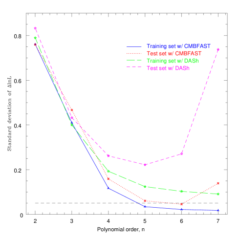
This approach is illustrated for the 6 parameter $\Lambda$CDM case in figure 1, where we plot the fitting accuracy for 2nd through 7th order polynomials, showing the difference between test and training sets. The training set errors predictably fall with increasing polynomial degree, as there are more degrees of freedom with which to fit the data. The test set errors, however, have a clear minimum (in this case for $n=6$) which is what we choose as optimal polynomial fit. This optimal polynomial degree depends strongly on how long a chain is used for the fit. A large sample allows us to go to higher order, whereas for a small sample, even 3rd or 4th order polynomials may be ill fated.

Due to theoretical prejudice for the probability distributions to be close to Gaussian as well as relatively smooth, it is possible that some of the errors in fitting to the CMBfast-calculated likelihoods could be due to inaccuracies in CMBfast itself rather than our polynomial approximation. although we have not attempted to test or quantify this, this may be worth exploring in future work.

Figure 1 also shows that we obtained slightly larger random scatter when computing power spectra with DASh [27] instead of CMBfast. This does not to appear to be a limitation of DASh itself, since the accuracy is greatly improved when using the latest version of DASh with transfer functions from the latest version of CMBfast (Knox 2003, private communication). From here on, we use CMBfast to calculate all our likelihood samples.

FIG. 1.: R.m.s. fitting error $\Delta\ln{\cal L}$ for the 6 parameter $\Lambda$CDM case. The plot compares the training and test sets for fits based on chains using CMBfast and chains using DASh. For the particular chain-length used for the CMBfast case, we see that a 6th degree fit is optimal.

The mean scatter in the values of $\ln{\cal L}$ range from a good $0.05$ for the 6th order fit to the $\Lambda$CDM 6 parameter model to a more dubious $0.69$ for the 6 parameter + tensor perturbation case. Accuracies for all the cases are shown in table II. However it is not immediately clear that the error in $\ln{\cal L}$ is necessarily the most interesting quantity, as it may include contributions at low $\ln{\cal L}$ which will have negligible impact on the relevant parts of the likelihood surface.

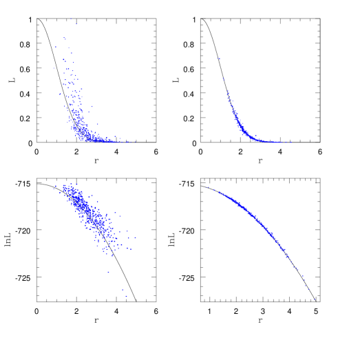
An equally interesting quantity is $\Delta{\cal L}={\cal L}_{fit}-{\cal L}$ (we normalize ${\cal L}$ to equal unity at its maximum), which shrinks rapidly with decreasing values for $\ln{\cal L}$ and thus better illustrates what kind of accuracies we can expect for the marginalized distributions. The mean scatter in the values of ${\cal L}$ are significantly smaller, typically of order $\sim 0.01$ for the entire dataset. A better understanding of these quantities can be obtained by studying figure 2. It shows first how well (or rather how badly) the actual likelihood surface (both in terms of ${\cal L}$ and $\ln{\cal L}$) is described by a Gaussian PDF in the transformed normal parameters. These are the variables ${\bf z}$ defined in section II C, which have zero mean and identity covariance matrix, and the $d$-dimensional radius is given by $r=|{\bf z}|=(z_{1}^{2}+\cdots+z_{d}^{2})^{1/2}$. The plot then shows the fitting errors $\Delta{\cal L}\equiv{\cal L}_{fit}-{\cal L}$ and $\Delta\ln{\cal L}=\ln{\cal L}_{fit}-\ln{\cal L}$, plotted as errors relative to a Gaussian distribution. This visualizes the ability of the method to reproduce the likelihood surface with good precision and the dramatic improvement gained from going to polynomial degree higher than two.

FIG. 2.: The accuracy of our method for the case of a 5th order polynomial fit to the 7-parameter case including $\alpha$ is shown for the likelihood ${\cal L}$ (top) and its logarithm $\ln{\cal L}$ (bottom). The left panels show how well the likelihood is fit by a pure Gaussian, as a function of the radius $r$ in the transformed parameter space. The right panels show the corresponding errors $\Delta{\cal L}\equiv{\cal L}_{fit}-{\cal L}$ (top) and $\Delta\ln{\cal L}\equiv\ln{\cal L}_{fit}-\ln{\cal L}$ for our polynomial fit, plotted relative to the Gaussian, i.e., the top right panel shows ${\cal L}_{gauss}+{\cal L}_{fit}-{\cal L}$.

Model	Chain origin	Chain length	Priors	Pol. deg. $n$	$\Delta\ln{\cal L}_{train}$	$\Delta\ln{\cal L}_{test}$
6 par T	Own	183008	None	6	0.02	0.08
6 par T+X	Own	311391	None	6	0.02	0.05
6 par + $k$	WMAP	278325	$\tau<0.3$	4	0.25	0.36
6 par + $\alpha$	WMAP	435992	$\tau<0.3$	4/5	0.12/0.08	0.14/0.12
6 par + $r$	Own	178670	None	4	0.29	0.69

TABLE II.: R.m.s. polynomial fit errors for all the considered cases, ranging from 6 parameter vanilla $\Lambda$CDM models to spiced up models including curvature, tensor perturbations, running tilt.

B Application to MCMC

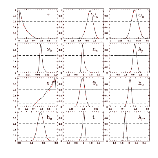
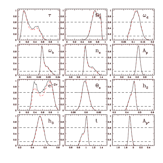
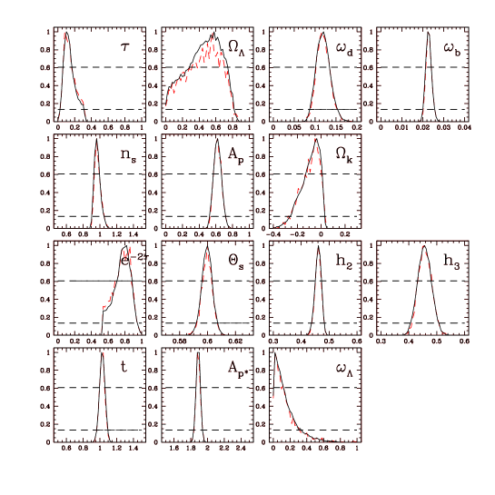
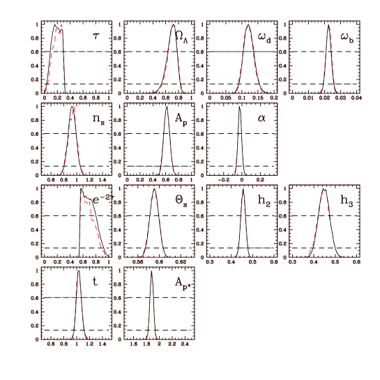
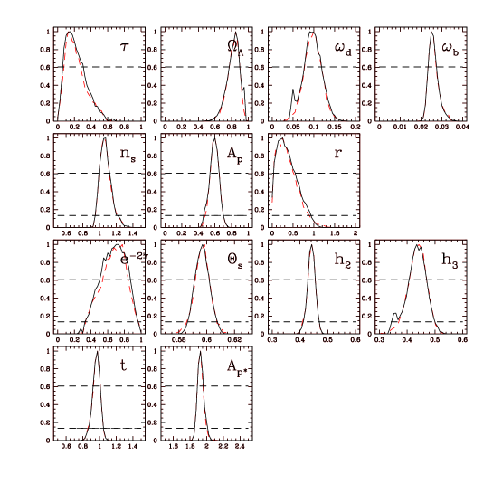
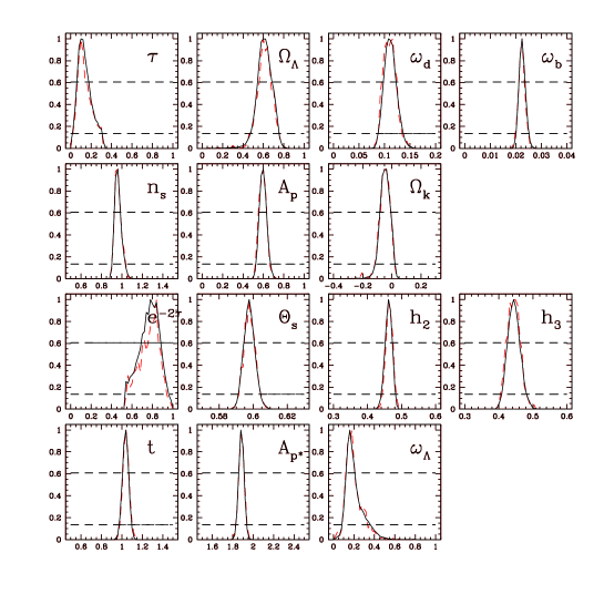
The ultimate end-to-end test of the method is how well the 1-dimensional and 2-dimensional marginal distributions are reproduced. To test this, we use the polynomial fits to calculate the likelihoods for our MCMC algorithm. Due to the inevitability of polynomial artifacts at low confidence areas, we use a cut-off at the 3 sigma level (corresponding to a maximum value for $r$ defined above), where we replace the polynomial fit by a simple Gaussian. This allows for the algorithm to find its way through the burn-in process to the allowed part of parameter space from any starting point. The results are shown in figures 3-7. The figures show what is already indicated in table II: The marginalized distributions are reproduced to well within the sampling errors, the only exceptions being a couple of parameters in the tensor case, demanding only negligible computational time (a chain of length 200000 runs in about a minute).

Figure (8) illustrates one of the most useful applications of our approach: combining WMAP with another data set, here the SDSS galaxy power spectrum as reported in [7, 8] to give constraints on the cosmological parameters for a non-flat 7 parameter model. The red dashed curve shows the results from running a Markov Chain Monte Carlo for about a week obtaining only 14000 points, and the solid black curve is the reproduction by our polynomial fit, taking a mere afternoon to run. Indeed, the time-consuming part in this calculation was the computation of the non-linear matter power spectrum, the processor time needed to calculate the WMAP likelihoods being under a minute.

FIG. 3.: WMAP 6 parameter $\Lambda$CDM case, using only the WMAP temperature power spectrum. We show marginalized likelihoods for the polynomial fit compared to the original chain. The two chains are indistinguishable.

FIG. 4.: WMAP $\Lambda$CDM T+X case, marginalized likelihoods for the polynomial fit plotted on top of the ones from the original chain. The two chains are nearly indistinguishable apart from a small difference in fitting the second (and otherwise ruled out) peak in the optical depth distribution.

FIG. 5.: WMAP $\Lambda$CDM + curvature case, marginalized likelihoods for the polynomial fit compared to the original chain. Again we see two almost identical sets of distributions, apart from some poisson noise in the original chain.

FIG. 6.: WMAP $\Lambda$CDM + running scalar tilt, marginalized likelihoods for the polynomial fit compared to the original chain. Apart from minor differences in the $\tau$ distribution, the two distributions are identical.

FIG. 7.: WMAP $\Lambda$CDM + tensor case, marginalized likelihoods for the polynomial fit plotted over the ones from the original chain. The difficulty in fitting this case is seen in the unphysical polynomial artifacts shown in the distributions for $\omega_{d}$ and $h_{3}$. This effect is removed when adding the SDSS data.

FIG. 8.: SDSS + WMAP $\Lambda$CDM + curvature contributions, marginalized likelihoods for the polynomial fit compared to a chain consisting of only $\sim 14000$ points. The fit is excellent, the errors coming from poisson noise due to the short length of the CMBfast calculated chain.

IV Conclusions and Discussion

The big bottleneck in parameter estimation with CMB data has hitherto been the computation of theoretical power spectra by means of CMBfast, CAMB, CMBEASY, DASh or similar, for a reasonably fast computer typically requiring from $~{}5$ seconds to several minutes for non-flat models with massive neutrino for CMBfast, and $~{}1$ second for DASh. In contrast, our method requires less than a millisecond per model, since we have already precomputed the WMAP likelihoods using CMBfast and distilled the results into a convenient fitting function. After transforming into a physically motivated parameter set, the only calculation needed is the evaluation of an $n^{th}$ order polynomial with as few as 210 coefficients for the 6 parameter quartic case. As the number of coefficients may actually exceed the number of measured $C_{l}$s the method is clearly not a way of compressing the data. Rather we are compressing the amount of calculation necessary to convert cosmological parameters into likelihood values.

The typical error in this approach is $\Delta{\cal L}\sim 0.01$ (with the peak likelihood normalized to unity) and $\Delta\ln{\cal L}\sim 0.05-0.5$. To place these inaccuracies in context, let us first discuss how they compare with the inaccuracies in other methods, then the question of how good is good enough.

The latest version of CMBfast[23] has an accuracy down to $\sim 0.1\%$ (r.m.s). It is unclear if other recent packages match this number, but they are generally good to the $1-2\%$ level. Despite computer advances, the CMBfast code is still slow when several hundred thousand model computations are required as for grid calculations or Markov Chain Monte Carlo applications. Several shortcuts have therefore been developed in order to compute the Likelihood faster than the full CMBfast. The “$k$-split” method in CMBfast due to Tegmark et al. [26] utilizes the fact that the high-$\ell$ and low-$\ell$ ends of the power spectrum depends on different parameters, and so calculates the two parts separately. The end result is then combined into a final power spectrum. The Davis Anisotropy Shortcut (DASh)[27] takes this method further, and creates the power spectrum by interpolation between points in a huge pre-computed grid of transfer functions. Comparing likelihoods calculated with $k$-split CMBfast and DASh with those calculated with the maximally accurate CMBfast, we found that the errors from our fitting method in both $\Delta\ln{\cal L}$ and $\Delta{\cal L}$ are significantly smaller than the errors in these quantities from the DASh or $k$-split approximations. For instance, DASh gave r.m.s. $\Delta\ln{\cal L}\approx 0.9$ for the 6-parameter case using only unpolarized WMAP information and the ksplit inaccuracies are similar, which should be compared with our value $\Delta\ln{\cal L}\approx 0.08$ from Table II.

How accurate is accurate enough? For most applications, the key issue is not inaccuracies in the power spectra or likelihoods, but inaccuracies in measured cosmological parameters. If an approximation shifts the measured values of all parameters by much less than their statistical uncertainties, it is for all practical purposes irrelevant.

We have also shown that the errors in the marginalized distributions are minimal, and that our method should be used by anyone who do not have excessive amounts of time and computer power on their hands. Our last six figures show that our approximation is clearly accurate enough in this sense except for the above-mentioned glitches in the tensor case. There is, however, one subtle and somewhat counterintuitive point that is worth clarifying. Since WMAP constrains the power spectrum normalization to the $10^{-3}$ level when all other parameters are held fixed, this means that even a seemingly tiny $\sim 0.1\%$ inaccuracy in the power spectrum can in principle cause a change of order unity in $\chi^{2}$ and $\Delta\ln{\cal L}$, i.e., an inaccuracy larger than that of our fitting method, and one may naively expect that inaccuracies of order $\Delta\ln{\cal L}\sim 1$ would affect the parameter measurements at the $1\sigma$ level. Although this would be true if only one parameter were being measured, the situation at hand is actually much better because of degeneracies. As long as the inaccuracies do not exactly mimic the effect of changing some cosmological parameter, they will alter $\ln{\cal L}$ mainly via the narrowest directions in the multidimensional degeneracy banana and hence have little effect on the final results. For instance, if a fitting inaccuracy causes a relative error in $\Theta^{E}_{s}$ at the $10^{-3}$ level, it will have no noticeable effect on the estimates any of the vanilla cosmological parameters, whose error bars are dominated by the eigenparameters with the largest rather than the smallest uncertainties. The bottom line is therefore that although the the DASh and $k$-split $\ln{\cal L}$ inaccuracies of order unity may sound worrisome, these two approximations are nonetheless sufficient to give negligible inaccuracies in cosmological parameter measurements, and the still better accuracy of our fitting method is actually overkill.

Our method has several applications. First, it is extremely useful when combining the WMAP-data with non-CMB data such as the galaxy surveys, weak lensing data, supernovae data, etc., where likelihood calculations are fast relative to CMB power spectrum calculations. Using our method to measure parameters from the combined WMAP and SDSS data [8] enabled us to do some of the analysis with dramatically increased speed. Second, even when running Markov chains for models not considered here, one can get good results by simply running the chain for long enough to acquire a sufficient (but not necessarily statistically fair) sample of the surface, then compute the polynomial fit, and go on to use this fit for the remainder of the job — until all relevant mixing and convergence tests are fulfilled. A further obvious application is generating extremely long Markov chains, eliminating sampling errors almost completely. Finally, should the reader be intent on requiring the best accuracy that CMBfast can offer, our approach can still be helpful: It is a fundamental fact about MCMC algorithms that they do not produce completely uncorrelated points, and the correlation length of the chains can easily be several hundred points, and only gets as low as 45 even for our simply 6-parameter WMAP chains. Thus the calculations may be significantly accelerated by creating a statistically random sample by means of the polynomial fit, thinning the chain to every 200 points or so, and calculating the CMBfast power spectrum and WMAP likelihoods for these points. A final likelihood sample with the strictly correct distribution may then be obtained using importance sampling as described in [32].

We supply Fortran routines for computing the likelihoods for all the cases given in the text at http://www.hep.upenn.edu/$\sim$sandvik/CMBfit.html , and we plan to complement this work with further models and fits in the future.

V Acknowledgements

We wish to thank L. Verde and the rest of the WMAP team for kindly supplying us with the Markov chains from their analysis. HS wishes to thank R. Jimenez and P. Protopapas for valuable discussions. This work was supported by NSF grant AST-0134999, NASA grant NAG5-11099 and fellowships from the David and Lucile Packard Foundation and the Cottrell Foundation.

REFERENCES

- [1] C.L. Bennett et al., ApJS, 148, 1 (2003)
- [2] G. Hinshaw et al., ApJS, 148, 135 (2003)
- [3] A. Kogut et al., ApJS, 148, 161 (2003)
- [4] L. Page et al., ApJS 148, 233 (2003)
- [5] D. N. Spergel et al., ApJS 148, 175 (2003)
- [6] L. Verde et al., ApJS 148, 195 (2003)
- [7] M. Tegmark et al. astro-ph/0310725
- [8] M. Tegmark et al. astro-ph/0310723
- [9] D. Eisenstein , W. Hu and M. Tegmark, Astrophys.J. 518 (1998) 2-23
- [10] J.L. Tonry et al. ApJ, 594,1 (2003)
- [11] S.Bridle, O.Lahav, J.P.Ostriker and P.J.Steinhardt, 2003, Science, 299, 1532
- [12] M. Tegmark, Phys. Rev. D55, 5895 (1997)
- [13] J.R. Bond and G. Efstathiou, MNRAS 226,655 (1987)
- [14] J.R. Bond, A.H. Jaffe and L. Knox, Phys. Rev. D57, 2117 (1998)
- [15] B.D. Wandelt, D.L. Larson and A. Lakshminarayanan, astro-ph/0310080 Phys. Rev. D 55, 5895 (1997) [arXiv:astro-ph/9611174].
- [16] J.R.Bond, A.F.Jaffe and L.E.Knox, Astrophys. J. 533, 19 (2000) astro-ph/9808264
- [17] A.F. Jaffe, J.R.Bond, P.G. Ferreira and L.E. Knox, astro-ph/0306506
- [18] W.Hu, M.Fukugita, M.Zaldarriaga , M.Tegmark, Astrophys.J. 549 (2001) 669
- [19] W.Hu and N.Sugiyama, Phys. Rev. D 51, 2599 (1995)
- [20] A. Kosowsky, M. Milosavljevic and R. Jimenez, Phys. Rev. D 66, 063007 (2002) [arXiv:astro-ph/0206014].
- [21] M. Chu, M. Kaplinghat and L. Knox, arXiv:astro-ph/0212466.
- [22] U.Seljak and M. Zaldarriaga, Astrophys.J. 469 (1996) 437-444
- [23] U.Seljak, N.Sugiyama, M.White, M.Zaldarriaga, astro-ph/0306052
- [24] A.Lewis, A.Chalinor and A.Lasenby, Astrophys.J. 538 (2000) 473
- [25] X.Wang, M. Tegmark and M. Zaldarriaga, Phys.Rev. D65 (2002) 123001
- [26] M.Tegmark, M.Zaldarriaga, A.J.S.Hamilton, Phys.Rev. D63 (2001) 043007
- [27] M. Kaplinghat, L. Knox and C. Skordis, Astrophys. J. 578 (2002) 665 [arXiv:astro-ph/0203413].
- [28] M.Doran, astro-ph/0302138
- [29] M.Doran, et.al., astro-ph/0012139
- [30] M.Doran and M.Lilley, astro-ph/0104486
- [31] D.J.C.MacKay Information theory, inference and learning algorithms, Cambridge University Press (2003)
- [32] A. Lewis and S. Bridle, Phys.Rev. D66 (2002) 103511
- [33] L. Knox, N. Christensen and C. Skordis, ApJ, 578, L95 (2001)
- [34] N.Christensen and R.Meyer, astro-ph/0006401
- [35] N.Metropolis, A.W.Rosenbluth, M.N.Rosenbluth, A.H.Teller and E.Teller, J.Chem.Phys. 21 (1953) 1087
- [36] W.K.Hastings, Biometrika 57 (1970) 97
- [37] W.R.Gilks, S.Richardson and D.J.Spiegelhalter;1996;Markov Chain Monte Carlo in Practice;Chapman & Hall;London
- [38] A.Gelman and D.Rubin, Statistical Science 7 (1992) 457
- [39] N.Christensen, R.Meyer, L.Knox and B.Luey, Class. Quant. Grav. 18 (2001) 2677
- [40] A.Slosar and M.Hobson, (2003), astro-ph/0307219
- [41] O.Zahn and M.Zaldarriaga, PRD 67 (2003) 63002
- [42] S.Dodelson, Modern Cosmology, Academic Press, 2003