Exponential Potentials for Tracker Fields

Abstract

We show that a general, exact cosmological solution, where dynamics of scalar field is assigned by an exponential potential, fulfils all the issues of dark energy approach, both from a theoretical point of view and in comparison with available observational data. Moreover, tracking conditions are discussed, with a new treatment of the well known condition $\Gamma>1$. We prove that the currently used expression for $\Gamma$ is wrong.

I Introduction

A Motivations

The recent discovery of the acceleration of the Universe [1, 2] has produced an overwhelming number of papers on its possible explanations, alternative to a plain cosmological constant (see Refs. [3, 4, 5] for reviews). Historically, the most favourite one is the introduction of a scalar field, usually minimally coupled with gravity (but see Refs. [6, 7, 8, 9, 10, 11, 12, 13] for other possible models). This poses the problem of the choice of a suitable potential. Moreover, as the equations are not exactly solvable in general, there is also a problem of qualitative analysis of the solutions and of the choice of initial conditions. Usually, very crude approximations are made, first of all the socalled “slow roll” condition, i.e., $\dot{\varphi}^{2}\ll V(\varphi)$.

The aim of this paper is to illustrate some subtleties involved by this situation, by means of a complete treatment of the general exact solutions of the Einstein equations in presence of both nonrelativistic matter and scalar field, with a suitable physical potential, and with a new treatment of the well known “tracking condition”, $\Gamma>1$ .

One result is that the slow roll condition is indeed not necessary and that insisting on it can bring to lose very interesting models; closely connected to this, is a discussion on the meaning of the statement that the state equation $w\equiv p_{\varphi}/\rho_{\varphi}$ for the scalar field should be “almost constant”. By means of an analytic example, we shall see that this expression is highly misleading, indeed.

Our choice for the potential is a particular class of exponential functions

$$V(\varphi)=B^{2}e^{-\sigma\varphi}\,,$$ (1)

with $B$ arbitrary and $\sigma\equiv\sqrt{3/2}$ (in units $8\pi G=1$). The reason for this special choice will be clear below.

First of all, we have to say that, although exponential potential is natural in higher dimension theories, supergravity and superstring models [14, 15, 16], it is not generally considered as feasible, even though it is often used at least as a first tool of analysis [17, 18, 19]. The usual objection to this potential is in fact that it cannot really be the right one, because “it scales approximately” like the matter component, so that, if the dark energy is dominant now, it should have been dominating also in the past, which is in contrast with BBN observations [20]. This potential was nonetheless proposed by some of us in Ref. [21], where also some explanations of the reason why this is not true in our case are given. Anyway, in Sec. III the problem is fully explored, and we show why the above objection is wrong.

A second common objection is that it describes a very peculiar situation, due to a fine tuning of initial conditions. We insist on the point that the solution found in Ref. [21] is general and exact. Here, we start indeed from a particular choice, but then we go further and release it, showing that the same “final situation” is reached, starting from a wide set of “initial conditions”. Again, we use quotation marks because the expressions are ambiguous and misleading, so that a preliminary discussion is needed to clarify what we mean.

A third possible objection is that this model could be in contrast with the observations. As a matter of fact, some papers have already appeared, successfully comparing this model with present day observations [22, 23, 24]. In Sec. II.B a first comparison with observational data is made, with very encouraging results. However, this paper is mainly concentrated on theoretical discussion. Our purpose is to show that the model we consider can emulate very well a standard model with dust plus a cosmological constant, well beyond any reasonable improvement of the observational techniques. In order to do this, a preliminary discussion on what is really measurable is again needed.

A second important result of our considerations consists in showing that many of the current statements about tracking solutions are based on an incorrect result and should therefore be revisited.

The paper is organized as follows. First, we examine some issues usually investigated when building a cosmological model with dark energy; key features like cosmic components, choice of the scalar field potential, measurability, and tracking behavior are therefore shortly sketched. Sec. II is then devoted to the exponential potential case and the general, exact solution that can be given to the cosmological equations. A comparison with a constant $\Lambda$ model and observational data is made; also, there can be found an analysis of the scalar field equation of state and a more detailed one of the tracking behavior. In Sec. III, the features usually assigned to the tracking notion are critically examined, giving new insights into such a concept. Finally, concluding remarks are drawn in Sec. IV.

B Preliminary discussion

First of all, before going through the analysis of our potential, we think it is useful to discuss some general questions which should be of help in understanding better what follows.

1 How can we set the choice for the potential?

At the moment there is no idea of which form the potential of the scalar field should take. The widely discussed inverse power law [5, 25], for instance, is certainly useful for a qualitative treatment of the problem, but only under the assumption of the slow rolling condition. It seems that the answer to this problem is simple in principle: the right form is the one that gives the best fit to the observed luminosity distance curve $d_{L}(z)$, and the fact that we cannot establish it firmly is only due to our limited observational precision. Indeed, it is possible to show that, whichever is the expression of $d_{L}(z)$, we can find, in principle, a suitable form for $V(\varphi)$, which gives it back. Unfortunately, the value of $\Omega_{0m}$ turns out to be arbitrary! The reason of this is due to the fact that the introduction of an arbitrary function in the model is equivalent to taking an infinite number of free parameters into account. Worst of all, this result is possible only if one has the exact functional form of $d_{L}(z)$. This is clearly impossible without already having a model in mind, so that one is led again at the starting blocks [26, 27, 28, 29, 30].

In our opinion, the only possible way to escape from this impasse is to ask for potentials which have some possible explanation in terms of fundamental physics or which exhibit some nice mathematical feature, which at least leaves the hope that it is due to some still unknown fundamental physical property. As for the first requirement, to our knowledge, the best candidates are the exponential potential, like that in Eq. (1) (but with $\sigma$ undetermined), and polynomials of the form

$$V(\varphi)=\frac{1}{2}m^{2}\varphi^{2}+\lambda\varphi^{4}+\text{{hig. ord.}}$$ (2)

It is important to observe, however, that this is a generic expansion of an even function $f(\varphi)$, with a suitable minimum, so that any function of this type will be good as well.

As for the second requirement, we shall see below that the potential proposed in Eq. (1), due to the special value of $\sigma$, exhibits a Noether symmetry in the equations, which is just the reason why exact integration is possible. Also, the potential of Eq. (2) can be seen as the expansion of a generalized hyperbolic sine, with the same type of symmetry [31] (see below).

On the other hand, it is also possible to show that a sum of exponentials of the class in Eq. (1) plus a cosmological constant is essentially the most general type which can lead to exact integration in elementary way [32].

2 What is really measurable?

In the context chosen by us, we have a two-dimensional configuration space, with variables $\left\{a,\varphi\right\}$ plus the velocities $\left\{\dot{a},\dot{\varphi}\right\}$, so that the total number of variables is four. Consequently, this is the maximum number of independent quantities which can be measured. As a matter of fact, none of these quantities is in fact practically measurable. In flat cosmologies, $a_{0}$ is not measurable in principle. This is connected with the choice $k=0$, i.e., in terms of measurable quantities, $\Omega_{tot.}=1$ exactly, which is clearly artificial. Instead of these rather abstract objects, we can also use derived quantities. One of them is, of course, $\Omega_{0m}$. This parameter is very important, not only for its physical meaning, but also because its value can, in principle, be measured independently from the SNIa observations [33]. Much has also been said about the value of the acceleration parameter $q_{0}$; but, again, it is not directly measurable in practice. However, $q_{0}$ is also present in the second term of the series

$$d_{L}(z)=H_{0}^{-1}\left(z-\frac{(1-q_{0})}{2}z^{2}+...\right)\text{ }\,,$$ (3)

so that it seems possible to measure it, after all. Unfortunately, truncation of Eq. (3) after the second term is valid only at rather low redshifts (say $z\leq 0.1$). At these values, it is practically impossible to obtain sufficient precision, while at higher values the other terms cannot be neglected.

What is thus left? It seems reasonable to stick to what is for the moment firmly established, i.e., $h\approx 0.7$ and $\Omega_{0m}\approx 0.3$, with $3\sigma$ level $\sim\!10\%$ and $\sim 50\%$ errors, respectively. If we are very optimistic, we can expect an improvement of precision in the future of a factor 5, say. We shall see that even this could be not enough to discriminate among models.

Also, a third useful variable could be the age of the universe $t_{0}$, for which we have only a rather poor estimate $t_{0}>12$ Gyr.

3 Which is the precise meaning of the expression “tracking behavior”?

One of the greatest advantages of the introduction of a scalar field consists in the possibility to avoid the fine tuning of initial conditions, obtaining the same final behavior “for a wide range of initial possibilities”. The last sentence is intentionally rather ambiguous. In fact, the situation is often depicted as “similar but not exactly equal” to that of an attractor in the theory of dynamical systems.

Let us thus try to be more precise. The equations which we have to consider are the Einstein equations plus the Klein-Gordon equation for the scalar field (for sake of simplicity we write them directly in the flat case, but the following argument holds in the general case as well)

$$3H^{2}=\rho_{\varphi}+\rho_{m}\text{ },$$ (4)

$$2\frac{\ddot{a}}{a}+\left(\frac{\dot{a}}{a}\right)^{2}+\frac{1}{2}\dot{\varphi}^{2}-V(\varphi)=0\text{ }\,,$$ (5)

$$\ddot{\varphi}+3H\dot{\varphi}+V^{\prime}(\varphi)=0\text{ }\,.$$ (6)

Eq. (4) is a first integral of the other two. The integration constant is hidden into $\rho_{m}$. For instance, in the case of dust, we have $\rho_{m}=Da^{-3}$; again, the value of $D$ is not directly measurable, but we shall not in fact make use of this equation. Instead, we shall use Eqs. (5) and (6). The reason is that it can be shown that, when $\rho_{m}$ is related to a pure dust component, they are derived by the following Lagrangian [34, 35]

$$L=3a\dot{a}^{2}-\frac{1}{2}a^{3}\dot{\varphi}^{2}+a^{3}V(\varphi)\text{}\,.$$ (7)

Eq. (4) is then obtained as conservation of the energy function $E_{L}\equiv\left(\partial L/\partial\dot{a}\right)\dot{a}+\left(\partial L/\partial\dot{\varphi}\right)\dot{\varphi}-L$.

A first consequence of this fact is that Liouville’s theorem holds for this system. Thus, the phase space volume of possible initial conditions is conserved and has no attractors.

Nevertheless, the tracking behavior can be recovered by the following argument. Consider a set of independent variables for this system (not necessarily $\{a,\varphi,\dot{a},\dot{\varphi}\}$) and a volume of possible initial conditions. During the evolution, the volume is deformed, and it is possible that its projection on a two(three)-dimensional subspace converges to a point or a line. It is clear now that the result is strongly dependent on the choices of variables and projection. It is also clear that the gain in information on the variables of the subspace is compensated by a loss of information on the variables of the complement.

In our specific case we can take advantage of the fact that, as said above, only a part of the possible variables is practically measurable. Therefore we can make the usual choice for the subspace, i.e., consider $\{\log a,\log\rho_{\varphi}\}$, and show that, for a large set of initial conditions of these two variables, the orbits converge to a line. Another possibility is to consider $\{H,\Omega_{m}\}$, and check that the orbits converge to a point.

It is also clear that only observable quantities should be taken into account. For any other parameter the concept of fine tuning is, in our opinion, simply meaningless.

The situation is in fact rather involved and will be discussed in Sec. II.D, by means of an example.

We think that the concept illustrated above is the only one which is relevant for the solution of the coincidence problem. However, in the literature the term “tracking” is often used in a different meaning. The idea is that a large set of initial conditions should converge towards a nearly constant $w$, well before the present epoch, and maintain this condition forever. We shall show in Sec. II.C that this situation, although of course possible, is not at all necessary.

II The exponential potential case

Let us here introduce the exponential potential in the cosmological framework. As we shall see, in this case the equations are easily integrable, which allows many interesting considerations. (See Ref. [36] for a more general treatment). After finding the solution, we derive some consequences with respect to observational data and special features of quintessence field.

A The solution

As said above we start from Eqs. (5) and (6), with potential (1), and, due to the existence of a Noether symmetry, we choose to make the transformation of variables

$$a^{3}=uv\quad,\quad\varphi=-\frac{1}{\sigma}\log\frac{u}{v}\text{ }\,.$$ (8)

With these new variables, the Lagrangian (7) becomes

$$L=\frac{4}{3}\dot{u}\dot{v}+B^{2}u^{2}\text{ }\,,$$ (9)

and we see that the variable $v$ is cyclic, showing the existence of a Noether symmetry. The related conserved quantity is

$$F\equiv\frac{\partial L}{\partial\dot{v}}=\frac{4}{3}\dot{u}=\frac{1}{3}(6\dot{a}+\sqrt{6}a\dot{\varphi})(a\exp(-\sigma\varphi))^{1/2}$$ (10)

and makes the integration of the equations immediate, so that we get [21]

$$u=u_{1}t+u_{2}\text{ }\,,$$ (11)

$$v=\frac{1}{6}u_{1}\omega t^{3}+\frac{1}{2}u_{2}\omega t^{2}+v_{1}t+v_{2}\text{ }\,,$$ (12)

with $\omega\equiv\sigma^{2}B^{2}$. We thus have a general exact solution with four integration constants $u_{1}$, $u_{2}$, $v_{1}$, $v_{2}$. It is not easy to treat this solution in full generality, and, as we have seen, not very useful. We have, therefore, to make a clever choice.

First, we fix the origin of time by setting $a(0)=0$. This can be done in full generality. It is in fact important to observe that we are not really fixing an initial condition for $a$, since the model is not valid at initial singularity. The initial value of $a$ is fixed by the time $t_{in},$ which we choose for the beginning of validity of the model itself, and which is to some extent arbitrary. (See Sec. II.D for a discussion on this point.) Thus, we have to set $u_{2}=0$, or $v_{2}=0$. It is easy to convince oneself that it is arbitrary to decide which one. But in Ref. [21] we made more than this, and decided to set to zero both. For the moment we make the same choice, i.e., $u_{2}=v_{2}=0$. This in fact selects the tracking solution, but this will be better examined in Sec. II.D, where such a condition will be released.

The second condition which we set is $t_{0}=1$. That is, we fix the time scale by taking as unit the age of the universe. Indeed, as $t_{in}$ is unknown, this is not exactly the age of the universe, but the difference is irrelevant. In this way we get rid of a very badly known quantity. It would be possible, anyway, to avoid this condition, but we have checked that there is no substantial advantage.

The third condition is to set $a_{0}\equiv a(t_{0})=a(1)=1$. This is standard and fixes the normalization of $a$, according to the above discussion.

The last condition is to set $H(t_{0}=1)\equiv{\mathcal{H}}_{0}$. Due to the choice of $t_{0}$, this parameter is of order one, but it is not the same as the usual $h$. To be clearer, since we are using a more or less arbitrary unit of time, this parameter gives no information on the observed value for $H_{0}$, but, as we shall see, it actually fixes the value of $\Omega_{0m}$. An independent measure of $H_{0}$, together with the value of ${\mathcal{H}}_{0}$, gives the age of the universe for this model.

The relevant physical quantities are then

$$H=\frac{\left(12{\mathcal{H}}_{0}-8\right)t^{2}+8-6{\mathcal{H}}_{0}}{\left(9{\mathcal{H}}_{0}-6\right)t^{3}+\left(12-9{\mathcal{H}}_{0}\right)t}\text{ }\,,$$ (13)

$$\Omega_{m}=\frac{\left(4-3{\mathcal{H}}_{0}\right)\left(\left(3{\mathcal{\ H}}_{0}-2\right)t^{2}-\left(3{\mathcal{H}}_{0}-4\right)\right)}{\left(2\left(3{\mathcal{H}}_{0}-2\right)t^{2}-\left(3{\mathcal{H}}_{0}-4\right)\right)^{2}}\text{ }\,,$$ (14)

$$w=-\frac{2\left(3{\mathcal{H}}_{0}-2\right)t^{2}+3\left(4-3{\mathcal{H}}_{0}\right)}{4\left(3{\mathcal{H}}_{0}-2\right)t^{2}+3\left(4-3{\mathcal{H}}_{0}\right)}\text{ }\,.$$ (15)

It is possible to see that the constant $u_{1}$ is present only in the expression of $\varphi_{0}$

$$\varphi_{0}=-\sqrt{\frac{2}{3}}\log u_{1}^{2}\,.$$ (16)

All the other quantities only depend on ${\mathcal{H}}_{0}$, so that it will also fix the values of $\Omega_{0m}$ and $w_{0}$ according to the equations

$$\Omega_{0m}=-\frac{2\left(3{\mathcal{H}}_{0}-4\right)}{9{\mathcal{H}}_{0}^{2}}\quad,\quad w_{0}=-\frac{8-3{\mathcal{H}}_{0}}{4+3{\mathcal{H}}_{0}}\,.$$ (17)

For ${\mathcal{H}}_{0}=1$, we have $\Omega_{0m}\approx 0.22$ and $w_{0}\approx-\,0.71$. These values are reasonable and in good agreement with the ones found in Ref. [22] for a best fit with SNIa data; they also agree at $1\sigma$ level with the values we will find below. Assuming $h=0.7$, we get $t_{0}\approx 15\,Gyr$, which is also good. Moreover, we get

$$\frac{\dot{\varphi}_{0}^{2}}{2V(\varphi_{0})}=\frac{1}{6}\text{ }\,,$$ (18)

showing that the slow rolling condition is not fulfilled, as said in the introduction.

When one is not interested in precise fits, but instead on qualitative analysis (like in Sec. II.D), it is useful to stick to these values, so that all the formulae get simpler. We thus get

$$a^{3}=\frac{t^{2}\left(t^{2}+1\right)}{2}\quad,\quad H=\frac{4t^{2}+2}{3t^{3}+3t}\quad,\quad\Omega_{m}=\frac{t^{2}+1}{\left(2t^{2}+1\right)^{2}}\quad,\quad w=-\frac{2t^{2}+3}{4t^{2}+3}\,.$$ (19)

B Comparison with $\Lambda$-term model and observations

We want, now, to show that our model is practically equivalent to a $\Lambda$-term model in accounting for present day observations. Since the aim of this paper is mainly theoretical, we present here only a preliminary check, postponing to a forthcoming paper a thorough treatment of various popular models.

In order to do this we take advantage of the CAMB [37] and CosmoMC [38] codes. The powerful CosmoMC algorithm allows to compare a model with the Wilkinson Microwave Anisotropy Probe (WMAP) [39] and CBI [40] data, as for the CMBR spectrum, and with SNIa data and other constraints coming from BBN and HST Key Project. The LSS power spectrum derived from the Two Degree Field (2dF) Galaxy Redshift Survey [41] is also taken into account.

In short the procedure consists in generating, from random sets of the parameters, thousands samples of results. The maximum likelihood is then obtained by product of the single likelihood functions as established by the observers teams. The details of the treatment can be found in Refs. [42, 43].

It is important to observe that the results are obtained by numerical integration of the equations, by means of a CAMB subroutine which includes radiation. This is necessary for generating CMBR spectrum, starting from the radiation dominated era. On the other hand, this should not affect the previous discussion, which in fact refers to a period well after decoupling. In any case, a first comparison of the effective $w$, ${\bar{w}}\equiv\int w\Omega_{m}da/\int\Omega_{m}da$, and of the function $w(a)$, obtained with numerical (including radiation) and analytical (without radiation) integrations of our model, gives perfectly overlapping results.

After running the program we obtain the best fit results reported in Table I. It is clear that the two sets of parameters are practically the same. Anyway, it is possible to compare the $\log(LH)$ values, from which it appears that our model is slightly, but of course not significantly, disfavoured.

Note that in our model it is possible to get an analytic parametric expression for the luminosity distance in terms of hypergeometric and Euler functions. We find

$$z=\left(\frac{2}{t^{2}\left(t^{2}+1\right)}\right)^{1/3}-1\,,$$ (20)

$$d_{L}(t,{\mathcal{H}}_{0}=1)=\frac{1}{\left(t^{2}+1\right)^{1/3}}\left(\frac{3\sqrt{\pi}\Gamma(7/6)}{\Gamma(2/3)t^{2/3}}-\frac{2^{2/3}\,_{2}F_{1}(1/6,1/3,7/6,-t^{2})}{t}\right)\,.$$ (21)

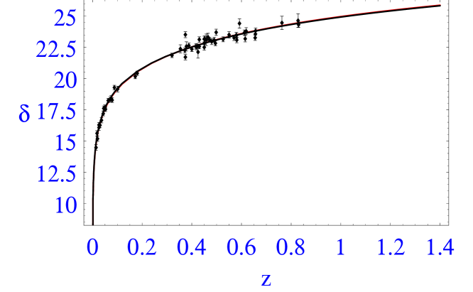
From this it is not difficult to compute the distance modulus and compare it with $\Lambda$-term model and SnIa data, which is done in Fig. 1.

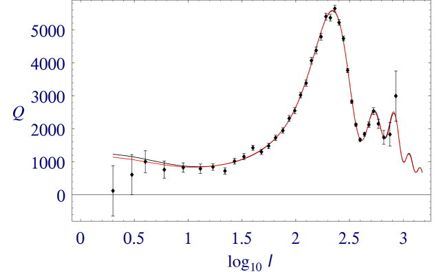
With the aid of CAMB code, we have also generated the CMBR spectrum for the two models, which is presented in Fig. 2.

The overlapping of the plots is striking in both cases. It is interesting to note that in this test we obtain equal values for $\Omega_{m}$ and marginally different values for $h$. In a previous test, based only on SnIa [22], we obtained instead very similar values for $h$ and quite different values for $\Omega_{m}$.

It appears very unlikely that more precise observations, of the same type here considered, will disentangle this degeneracy. An independent precise measure of $h$ and/or $\Omega_{m}$ could be, on the contrary, of great help.

C Analysis of $w$

Let us now analyze the variation of $w$, in order to understand better what was said in Sec. I.B.

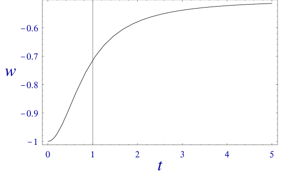
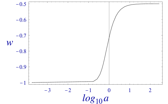
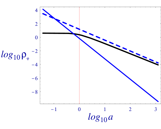
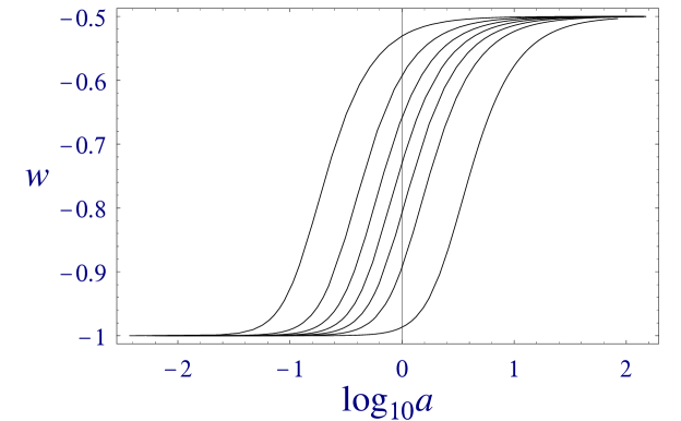
First of all, let us observe that the very notion of almost constant is somewhat ambiguous: we have in fact to ask almost constant with respect to which independent variable? We see from Fig. 3 that the function $w\left(t\right)$ does not show any flatness except towards infinity, which can be also easily deduced from Eq. (15). Quite different is the situation of $w\left(\log a\right)$, showed in Fig. 4. Here we have $w\sim-1$ in the past, with a sharp transition to the asymptotical value $w=-0.5$. What is most intriguing is the fact that the present time (i.e., $a_{0}=1$), marked by the vertical line, occurs just in the middle of this transition. Thus, we see that for the range of observational data, we have to consider the epoch when $w$ is mostly varying, that is, just the contrary of what is generally considered! The situation is illustrated also by the plot in Fig. 5, which contains the same type of information in a perhaps more familiar form.

Let us make some remarks on this point.

i) The situation just described looks like a striking cosmic coincidence, but we can show that it is not so striking. Indeed, the plot in Fig. 4 is done with the best fit values of Table I, but we can vary the present value of $\Omega_{0m}$ over a quite large range, much wider than any imaginable one, and obtain very similar results, as illustrated by Fig. 6.

ii) The above example shows that, in the context of our model, the allowed value of the parameter forces to place the present epoch in the period of maximal variability of $w$, with respect to $\log a$. If we consider another dependence, and of course if we change the model, this is not necessarily true.

iii) This example should indicate that the arguments involving variations of $w$ are really very subtle, and that it may be dangerous to base our conclusions on rough approximations based on this type of arguments.

D The tracking behavior

In this section, we release the condition $u_{2}=v_{2}=0$, which gave us the particular solution analyzed so far. As said above we can safely set $a(0)=0$, i.e., one of the two parameters $u_{2}$ or $v_{2}=0$. We have verified that it is better to set $u_{2}=0,$ since we get simpler formulae, which are rather complex anyway. Thus, since we are not interested here in best fit values, we set from now on directly ${\mathcal{H}}_{0}=1$, in order to obtain simpler expressions. As before, we also set in full generality $t_{0}=1$ and $a_{0}=1$, so that we are left with $u_{1}$ (as before) and $v_{2}$. Being it arbitrary, we pose $\varepsilon\equiv u_{1}v_{2}$, so that we have

$$u=u_{1}t\quad,\quad v=\frac{1}{6}u_{1}\omega t^{3}+v_{1}t+\varepsilon/u_{1}\,,$$ (22)

and, after evaluating $\omega$ and $v_{1}$ according to our conventions, we obtain for the relevant objects

$$a^{3}=\frac{1}{2}t^{2}(t^{2}+1)+\frac{1}{2}t(2-3t+t^{3})\varepsilon\,,$$ (23)

$$\varphi=\sqrt{\frac{2}{3}}\log\left(\frac{t+t^{3}+(2-3t+t^{3})\varepsilon}{2u_{1}^{2}t}\right)\,,$$ (24)

$$H=\frac{2}{3t}\frac{t+2t^{3}+(1-3t+2t^{3})\varepsilon}{t+t^{3}+(2-3t+t^{3})\varepsilon}\,,$$ (25)

$$w=-\frac{2t^{6}+3t^{4}+(4t^{6}-6t^{4}+8t^{3})\varepsilon+(2t^{6}-9t^{4}+8t^{3}-1)\varepsilon^{2}}{4t^{6}+3t^{4}+(8t^{6}-6t^{4}+4t^{3})\varepsilon+(4t^{6}-9t^{4}+4t^{3}-1)\varepsilon^{2}}\,,$$ (26)

$$\Omega_{m}=\frac{t(t^{3}+t)-t(2t^{3}+6t-2)\varepsilon-t(3t^{3}-9t+6)\varepsilon^{2}}{4t^{6}+4t^{4}+t^{2}+(8t^{6}-8t^{4}+4t^{3}-6t^{2}+2t)\varepsilon+(4t^{6}-12t^{4}+4t^{3}+9t^{2}-6t+1)\varepsilon^{2}}\,.$$ (27)

We see that, as before, $u_{1}$ alone only enters in the present value of $\varphi$, which is again given by Eq. (16). The observable quantities are now parametrized by $\varepsilon$, which must be small, if we want to recover the unperturbed solution discussed above. But it is important to say that, in our opinion, a small value of $\varepsilon$ should not be interpreted as a fine tuning on initial conditions. In fact, $\varepsilon$ is just a mathematical parameter; thus, according to what we said above, there is no point in discussing fine tuning of it. In any case, as we shall see just below, its value can span the range $0\div 10^{-9}$, so that it actually covers many orders of magnitude.

A second point must be discussed now. The presence of $\varepsilon\neq 0$, no matter how small, dramatically changes the solution near the singularity; we have indeed

$$\lim_{t\rightarrow 0}w=1\quad,\quad\lim_{t\rightarrow 0}\Omega_{m}=0\,,$$ (28)

and, depending on the value of $\varepsilon$, these conditions can be approximately maintained until a rather recent epoch. This is clearly not acceptable, and forces us to take very small $\varepsilon$, which sounds good. The problem is: how small? A reasonable answer seems to push the region where $w\approx 1$ farther than $z\approx 10^{3}$, i.e., before decoupling, where our model may be not good to work. We may consider, then, three possible strategies.

1) To be very restrictive and say that, before decoupling, the model is clearly not valid. In this way we shall see that we have no tracking behavior at all, but there is general agreement that convergence towards the tracking solution should begin before decoupling, so that this attitude does not bring us much farther.

2) To be less restrictive and say that the model can be anyway roughly good after equivalence, and just before decoupling. This corresponds to set the initial point somewhere between $z\approx 10^{3}$ and $z\approx 10^{4}$.

3) To be still less restrictive and say that, at least as toy model (i.e., as mathematical illustration of the situation), we can try to analyze what happens until nearby the initial singularity.

In the following we are discussing these two last situations, trying to clearly distinguish among them.

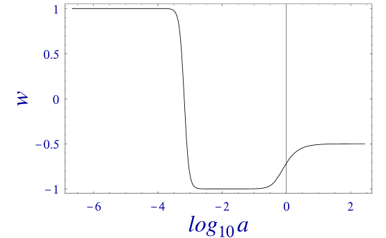
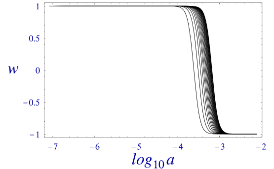
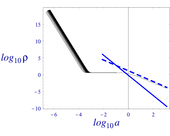
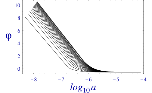
Let us start from Fig. 7, where we present the complete plot of $w$ versus $\log_{10}a$, for a particular very small value of $\varepsilon$. We see that the transition between $w\approx 1$ and $w\approx-1$ occurs at $z\approx 10^{3}$, as requested. Let us now vary $\varepsilon$ in the range $10^{-12}\div 10^{-9}$, which gives the plot in Fig. 8 (only the first transition is now shown). If we first adopt the point of view 2), we see that an almost complete set of values $w\in(-1,1)$ evolves towards $w=-1$ (and then the second transition), with irrelevant differences. The situation does not change if we adopt strategy 3), in which case however the Fig. 8 may be misleading. In fact, as $\varepsilon$ gets smaller and smaller, all the region with $w<1$ on the left should be filled with lines.

Now we pass to the more familiar plot of $\log_{10}\rho_{\varphi}$ versus $\log_{10}a$ (Fig. 9). Again, in the case 2), we can set the initial point between $z\approx 10^{3}$ and $z\approx 10^{4}$ and see that the values of $\log_{10}\rho_{\varphi}$ span the interval $(0,0.6)$, so that $\rho_{\varphi}$ can vary upon about $6$ orders of magnitude. This is not the hundreds of them presented in the literature, but we can recover this possibility just by adopting strategy 3). In this case, we have to consider all the triangle on the left until, say, the end of inflation.

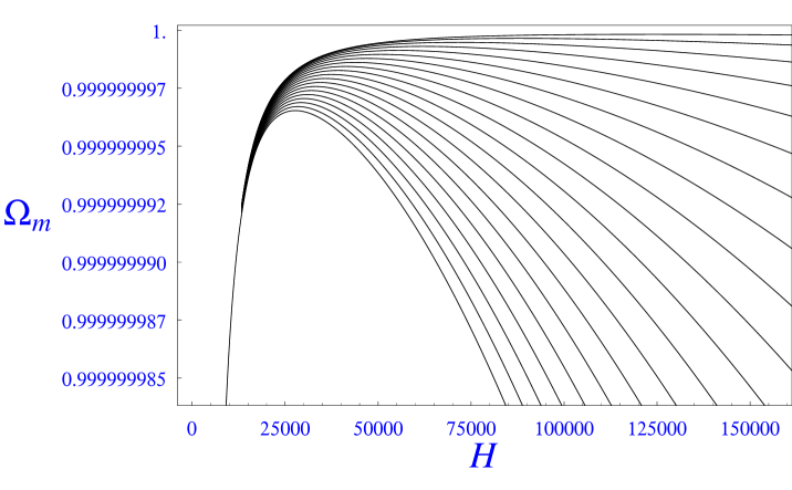
In Fig. 10 we present the plot of $H$ versus $\Omega_{m}$. The situation seems very similar to the others, with a lot of initial conditions converging towards the tracker solution. But, if you look at the values of $\Omega_{m}$ on the scale, all the values are indeed very close to $1$. Only if we adopt strategy 3) and go very far in the past, we get a somewhat larger set of initial values for this parameter. From a physical point of view this is good news, because we want $\Omega_{m}$ to dominate during the radiation epoch. This suggests that option 3) is not so bad, and indeed, as said before, a first verification on the function $w(a)$, obtained as a byproduct of CAMB integration including radiation, gives almost perfect concordance up to a redshift $\sim 10^{6}$.

From a pedagogical point of view, together with the above cases, we learn that the tracking behavior can be different, depending on which variables are taken into consideration, so giving strength to our initial consideration on the necessity to be very careful when treating this argument.

Needless to say, the tracking behavior will be completely lost if we consider the variable $\varphi$, and leave undetermined its present value. If we decide to fix it, which in principle can always be done, we have to set $u_{1}$ independently. If we set it to $1$ (but this is relevant only for numerical computation of the plot) and look at Fig. 11, for instance, the situation is quite similar to that of $\Omega_{m}$.

III The tracking concept revisited

We are now ready to analyze some widely accepted concepts about tracking solutions and understand some subtleties and incorrect results.

As said above, a currently accepted point of view on tracking solutions is that the ”attractor” should be characterized by a nearly constant value of $w$, well before the present epoch. Of course, it is true that the tracking solution must be reached before, but the above example should make it clear

i) that it does not imply $w$ being constant, while, on the contrary, the present epoch occurs in the period when $w$ changes most;

ii) that the asymptotic constant value has not necessarily anything to do with observations.

A second current point of view is that the potentials which are good for tracking should be such that

$$\Gamma\equiv\frac{VV^{\prime\prime}}{(V^{\prime})^{2}}>1\,,$$ (29)

with $\Gamma(\varphi)$ nearly constant over the possible range of $\varphi$. In this case, after some oscillations between $-1$ and $1$, $w$ should reach a stable nearly constant value, given by

$$w=\frac{w_{B}-2(\Gamma-1)}{1+2(\Gamma-1)}\,,$$ (30)

where $w_{B}$ is the state equation of the matter, in practice zero. This equation is derived from a well known formula [45].

Now, the only two potentials for which $\Gamma$ is strictly constant are the exponential ($\Gamma=1$) and the inverse power

$$V(\varphi)=M\varphi^{-\alpha}\,,$$ (31)

with $\alpha>0$ ($\Gamma=\left(\alpha+1\right)/\alpha$). In the first case, from Eq. (30) we get $w=w_{B}$, which seems to be untenable. In the second case, we have

$$w=\frac{\alpha w_{B}-2}{\alpha+2}\,.$$ (32)

These results have to be discussed and revised. So, let us first make the following four considerations.

1) In our example, the asymptotic value of $w$ is $\ -1/2$, so that, also in the case of practically constant $w$, it does not scale as the background. In fact, it is not difficult to show that, with a generic exponential potential $\ V=A\exp(-\lambda\varphi)$, a scaling equal to the matter background is possible only for $\lambda>\sqrt{3}$. This seems to be in contradiction with Eq. (30), which makes no distinction on the value of $\lambda$.

2) In the case of the double exponential of Eq. (37), it is easy to show that it is $\Gamma<1$ always, and yet it has proved to be suitable for tracking. This is not a contradiction with the tracking theorem, which only claims on sufficiency of $\Gamma>1$; but, as a matter of fact, a bad interpretation in the sense of necessity has driven the literature to neglect an interesting field of study.

3) In the case of Eq. (31), the system should evolve towards the value of Eq. (32), but in Ref. [46] they show that this value is maintained only for a short period, while the asymptotic value is $w=-1$. It is in fact not difficult to show that, if the scalar field dominates, and if there is a constant asymptotic value for $w$, this must be $-1$.

4) If we insert our exact solution into the expression of $\Gamma$ in Ref. [45], we do not find consistency!

We have thus worked out again the calculation for $\Gamma$, which is detailed in the Appendix, and found that the result in Ref. [45] is incorrect. The correct result is indeed the following

$$\Gamma=1-\frac{2}{1+w}\frac{{\tilde{\tilde{x}}}}{\left(6+\tilde{x}\right)^{2}}-\frac{1-w}{2\left(1+w\right)}\frac{\tilde{x}}{6+\tilde{x}}+3\frac{w_{B}-w}{1+w}\frac{1-\Omega_{\varphi}}{6+\tilde{x}}\,,$$ (33)

where

$$x\equiv\frac{1+w}{1-w}\quad,\quad{\tilde{x}}\equiv\frac{d(\log x)}{d(\log a)}\quad,\quad{\tilde{\tilde{x}}}\ \equiv\frac{d\,{\tilde{x}}}{d(\log a)}\,,$$ (34)

so that, in the case when $w$ is nearly constant, $\tilde{x}$ and ${\tilde{\tilde{x}}}$ can be neglected.

It is straightforward to check that this is consistent with our solution, but what is really important is that, if $w$ is nearly constant, Eq. (30) is not true. In the case of $w$ nearly constant, in fact, we have from the above equation that Eq. (30) must be substituted by

$$\Gamma\approx 1+\frac{w_{B}-w}{2(1+w)}(1-\Omega_{\varphi})\,,$$ (35)

and we find the answers to points 1) and 3). Indeed, if $w$ scales as $w_{B}$ (and we saw that this can be the case only for great values of the parameter $\lambda)$, then $\Omega_{\varphi}$ goes to a constant value $<1$, and everything is consistent; but, if the scalar field dominates and go faster forever, then $\Omega_{\varphi}\rightarrow 1$, so that $w$ can take any value. It can be indeed computed as [18]

$$w=\frac{\lambda^{2}-3}{3}\,.$$ (36)

We also see that, in the case of Eq. (31), since $\Omega_{\varphi}\rightarrow 1$, the only way to keep $\Gamma$ constant is to let $w\rightarrow-1$. In this case, however, the last terms in Eq. (33) cannot be neglected.

We thus see that, now, the picture is consistent. But Eq. (35) allows to obtain another interesting result. If there is a period in which $w$ is nearly constant and the scalar field ultimately dominates, then the asymptotic value for $\Gamma$ is $1$ and the potential is obliged to be exponential. However, we must note that this only means that the true potential approximates an exponential in the late evolution, without saying anything else on its analytical expression. In fact, a strictly constant $w$ implies an inverse hyperbolic sine potential [3, 47].

IV Conclusions

We have presented above a class of physically meaningful exponential potentials, which allow general exact solution of the Friedman and Klein-Gordon equations. We have also shown that this solution, in the limits of validity of the model, meets all the requests which are generally made for a quintessence model, except one: the possibility of switching off the acceleration in the future, which is needed for the asymptotic freedom of the model [48]. This can indeed be obtained by a modification of the potential.

One possibility, studied in Refs. [49, 50, 51], is to bring the value of $\sigma$ to the range $\sqrt{2}<\sigma<\sqrt{3}$, so that the limit value for $w$ is raised to a value greater than $-1/3$. Another possibility is to pass to a combination of exponentials, which we have treated in another paper [31].

This last example is particularly interesting, and it is worthwhile to summarize some results. Using the potential

$$V(\varphi)=(Ae^{\sigma\varphi/2}-Be^{-\sigma\varphi/2})^{2}\,,$$ (37)

it is possible to obtain essentially the same situation as shown here (with a simple exponential potential) for the past, until present epoch. Towards the future, instead, we get that $w$ oscillates forever between $-1$ and $1$, but the oscillations of $\rho_{\varphi}$ turn out to be damped, so that it effectively scales like matter, and dark energy never reaches complete domination of dynamics. (See Ref. [31] for details, and Ref. [52] for a closely related situation.)

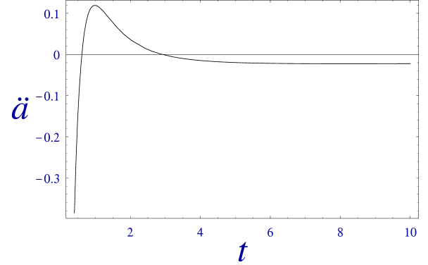
Coming back to the potential in Eq. (1), it is possible to guess a slightly positive spatial curvature. As said in the introduction, this is not excluded by the present data. It is then possible to add a curvature term into Eqs. (4), (5) and (6), and try to integrate them numerically. An appropriate choice for $\Omega_{k}$ gives the plot of Fig. 12, where we see that the acceleration starts from negative values, reaches a regime of positive values, and then goes back to negative in the future.

We have now to shortly discuss which are the shortcomings of the model we have considered so far in this paper.

First of all, although exponential potentials are widely considered as possible candidates to some kind of exotic dark energy (for physical reasons which are a priori with respect to the framework here presented), we have found no explanation which justifies the particular class of exponential potentials we have chosen, except the nice feature of the Noether symmetry of the Lagrangian (7) (but see Refs. [34, 35, 53, 54] for some discussion on this point).

Secondly, as we have repeatedly stressed, this model loses its validity when radiation is not negligible, and we have seen that a lot of interesting features occur just during that epoch. An extension is thus needed, but this must probably be done with numerical methods. Due to the very small values of some parameters, one must in fact be very careful to avoid numerical errors. In order to generate properly the plots of Sec. II, for instance, we had to work with $40$ digits floating numbers, and there was not cumulated error typical of numerical integration.

A study along these lines is presented in Ref. [51], where they find a behavior very similar to the one depicted by us for a reasonable range of values of $\sigma$ and initial conditions. They include radiation in numerical computation, but the procedure is somewhat different by ours.

Most of all, our discussion shows not only that this model can perfectly emulate a cosmological constant, but also gives no answers about the real possibility to discriminate, at least between these two models. It seems that we have shown that this discrimination is however impossible on the pure basis of luminosity distance observations. We have obtained this already known result [55] by showing that there is an important degeneracy in the $\Omega_{m}$ parameter.

In principle, this parameter can be measured independently, but it appears very difficult to reduce its present error of a factor, say, $10$ in the near future. We have also shown elsewhere that the two models are equally compatible with the observations on the peculiar velocities of galaxies [56]. This kind of measure is also affected by large errors, is time consuming and can say something only at rather low redshift ($z\approx 0.15)$. More promising seems to be the analysis of CMBR, as said above, and gravitational lensing, particularly of very distant QSO (see Ref. [57], for instance, and references therein). Here the problem appears to be the presence of a lot of other parameters, leading to huge degeneracy.

In our opinion, however, the main result which we obtain in this paper is probably pedagogical: we have learned that some statements, taken for granted by the majority of people, can be misleading. Let us summarize some of them here again.

We have seen that the most interesting epoch in our model is when $w$ is mostly variable, but only with respect to $\log a$. This shows that to say “ $w$ is necessarily almost constant” is badly stated, and risks to be merely a prejudice.

The study of the tracker behavior is subtle and strongly depends on the representation chosen. This is so even in the case when a general exact solution is given. This does not mean that qualitative analysis cannot be done in less favourable situations, but that it should be very carefully and unambiguously presented.

The requirement $\Gamma>1$ seems to be not necessary and, in any case, many widely accepted statements on exponential potentials and tracking solutions are indeed based on a result which has revealed to be incorrect.

In conclusion, we think that the final answer to the problem of the acceptable form for the potential is far to be reached, and that more insight on the physical motivations for the dark energy potential should be developed.

Let us rewrite Friedmann and Klein-Gordon equations

$$H^{2}=\frac{1}{3}\left(\rho_{B}+\rho_{\varphi}\right)\text{\quad},\text{ \quad}\dot{H}\equiv\frac{\ddot{a}}{a}-H^{2}=-\frac{1}{2}\left[\rho_{B}\left(1+w_{B}\right)+\rho_{\varphi}\left(1+w\right)\right]\,,$$ (38)

$$\ddot{\varphi}+3H\dot{\varphi}+V^{\prime}=0\,.$$ (39)

We then define as above

$$x\equiv\frac{\dot{\varphi}^{2}}{2V}=\frac{1+w}{1-w}\quad,\quad\tilde{x}\equiv\frac{d\ln x}{d\ln a}\ =\frac{\dot{x}}{Hx}\quad,\quad{\tilde{\tilde{x}}}\equiv\frac{d^{2}\ln x}{d\ln a^{2}}=\frac{1}{H}\frac{d}{dt}\left(\frac{\dot{x}}{Hx}\right)\,.$$ (40)

After substitution of

$$V^{\prime}\equiv\frac{dV}{d\varphi}=\frac{\dot{V}}{\dot{\varphi}}\quad,\quad V^{\prime\prime}=\frac{dV^{\prime}}{d\varphi}=\frac{1}{\dot{\varphi}}\frac{d}{dt}\left(\frac{\dot{V}}{\dot{\varphi}}\right)=\frac{\ddot{V}}{\dot{\varphi}^{2}}-\frac{\dot{V}\ddot{\varphi}}{\dot{\varphi}^{3}}$$ (41)

into the definition of $\Gamma$, we get

$$\Gamma=\left(\frac{\ddot{V}}{\dot{\varphi}^{2}}-\frac{\dot{V}\ddot{\varphi}}{\dot{\varphi}^{3}}\right)\frac{V\dot{\varphi}^{2}}{\dot{V}^{2}}=\frac{V\ddot{V}}{\dot{V}^{2}}+\frac{V}{\dot{V}\dot{\varphi}}\left(3H\dot{\varphi}+V^{\prime}\right)=\frac{V\ddot{V}}{\dot{V}^{2}}+3H\frac{V}{\dot{V}}+\frac{V}{\dot{\varphi}^{2}}\,.$$ (42)

Let us now compute the three terms of $\Gamma$. Starting from the last one, we have

$$\frac{V}{\dot{\varphi}^{2}}=\frac{1}{2x}=\frac{1-w}{2\left(1+w\right)}\,.$$ (43)

As for the second term, let us observe that

$$\frac{\dot{V}}{V} = \frac{d\ln V}{dt}=\frac{d}{dt}\left({2\ln\dot{\varphi}-\log 2-\log x}\right)$$ (44)

$$= \frac{2\ddot{\varphi}}{\dot{\varphi}}-\frac{\dot{x}}{x}=\frac{2}{\dot{\varphi}}\left({-3H\dot{\varphi}-V^{\prime}}\right)-H{\tilde{x}}$$ (45)

$$= -6H-\frac{\dot{V}}{xV}-H{\tilde{x}}\,,$$ (46)

so that we have

$$3H\frac{V}{\dot{V}}=-3\frac{1+x}{\left(6+{\tilde{x}}\right)x}=-\frac{6}{1+w}\frac{1}{6+{\tilde{x}}}\,.$$ (47)

Finally, let us compute the first term

$$\frac{V\ddot{V}}{\dot{V}^{2}}=\frac{V}{\dot{V}}\frac{d\ln\dot{V}}{dt}\,.$$ (48)

First, we have

$$\frac{d\ln\dot{V}}{dt}=\frac{\dot{V}}{V}+\frac{\dot{H}}{H}+\frac{\dot{x}}{x}+\frac{d{\tilde{x}}/dt}{6+{\tilde{x}}}-\frac{\dot{x}}{1+x}\,,$$ (49)

and, being

$$\frac{d{\tilde{x}}}{dt}=\frac{d}{dt}\left(\frac{\dot{x}}{Hx}\right)=H{\tilde{\tilde{x}}}\,,$$ (50)

we get

$$\frac{d\ln\dot{V}}{dt}=-\frac{6+{\tilde{x}}}{1+x}Hx+\frac{\dot{H}}{H}+H{\tilde{x}}+\frac{H{\tilde{\tilde{x}}}}{6+{\tilde{x}}}-\frac{{\tilde{x}}}{1+x}Hx\,.$$ (51)

From this relation, together with Eq.(47), we obtain

$$\frac{V\ddot{V}}{\dot{V}^{2}} = 1-\frac{\dot{H}}{H^{2}}\frac{1+x}{\left(6+{\tilde{x}}\right)x}-\frac{1+x}{x}\frac{{\tilde{x}}}{6+{\tilde{x}}}-\frac{1+x}{x}\frac{{\tilde{\tilde{x}}}}{\left(6+{\tilde{x}}\right)^{2}}+\frac{\tilde{x}}{6+{\tilde{x}}}$$ (52)

$$= 1-\frac{\dot{H}}{H^{2}}\frac{2}{1+w}\frac{1}{6+{\tilde{x}}}-\frac{1-w}{1+w}\frac{{\tilde{x}}}{6+{\tilde{x}}}-\frac{2}{1+w}\frac{{\tilde{\tilde{x}}}}{\left(6+{\tilde{x}}\right)^{2}}\,,$$ (53)

and, considering that

$$\frac{2x}{1+x}=1+w\,,$$ (54)

we find

$$\Gamma=1-\frac{2}{1+w}\frac{{\tilde{\tilde{x}}}}{\left(6+\tilde{x}\right)^{2}}-\frac{1-w}{1+w}\frac{\tilde{x}}{6+\tilde{x}}-\frac{6}{1+w}\frac{1}{6+\tilde{x}}\\ -\frac{\dot{H}}{H^{2}}\frac{2}{1+w}\frac{1}{6+\tilde{x}}+\frac{1-w}{2\left(1+w\right)}\,.$$ (55)

We have now to eliminate the term $\dot{H}/H^{2}$. From Eq. (38) it is

$$\frac{\dot{H}}{H^{2}} = -\frac{3}{2}\frac{\rho_{B}\left(1+w_{B}\right)+\rho_{\varphi}\left(1+w\right)}{\rho_{B}+\rho_{\varphi}}=-\frac{3}{2}\left(1+\frac{\rho_{B}w_{B}+\rho_{\varphi}w}{\rho_{B}+\rho_{\varphi}}\right)$$ (56)

$$= -\frac{3}{2}\left[1+\left(1-\Omega_{\varphi}\right)w_{B}+\Omega_{\varphi}w\right]=\frac{3}{2}\left[\Omega_{\varphi}\left(w_{B}-w\right)-\left(1+w_{B}\right)\right]\,,$$ (57)

and, by substitution, we eventually get

$$\Gamma=1-\frac{2}{1+w}\frac{\tilde{\tilde{x}}}{\left(6+\tilde{x}\right)^{2}}-\frac{1-w}{2\left(1+w\right)}\frac{\tilde{x}}{6+\tilde{x}}+3\frac{w_{B}-w}{1+w}\frac{1-\Omega_{\varphi}}{6+\tilde{x}}\,,$$ (58)

which should be compared with the formula reported in Ref. [45]

$$\Gamma=1+\frac{w_{B}-w}{2(1+w)}-\frac{1+w_{B}-2w}{2\left(1+w\right)}\frac{\tilde{x}}{6+\tilde{x}}-\frac{2}{1+w}\frac{\tilde{\tilde{x}}}{\left(6+\tilde{x}\right)^{2}}\,.$$ (59)

	$\Lambda$-term $-\log(LH)=765.3$			Exp. pot. $-\log(LH)=767.3$
par.	best fit	lower	upper	best fit	lower	upper
$\Omega_{b}h^{2}$	$0.0226$	$0.0206$	$0.0256$	$0.023$	$0.0213$	$0.0266$
$\Omega_{dm}h^{2}$	$0.120$	$0.103$	$0.139$	$0.110$	$0.094$	$0.134$
$n_{s}$	$0.960$	$0.914$	$1.05$	$0.948$	$0.905$	$1.04$
$\Omega_{m}$	$0.298$	$0.222$	$0.379$	$0.298$	$0.232$	$0.383$
$z_{re}$	$12.1$	$2.57$	$24.0$	$12.6$	$2.50$	$23.6$
$h$	$0.692$	$0.643$	$0.770$	$0.669$	$0.628$	$0.729$

TABLE I.: Best fit parameters for the two models. LH is the likelihood function obtained with the CosmoMC codes, as explained in the text. Caution must be paid in the interpretation of the lower and upper limits of the parameter values. They are not the $1\sigma$ constraints, but the extremal points of the $6$-dimensional confidence region. In any case, this table gives a clear indication that the two models are compatible with usual data. The small difference in the likelihood is not significant.

FIG. 1.: The distance modulus for the $\Lambda$-term and the exponential potential models, obtained from best fit parameters of Table I, is compared with SNIa Perlmutter at al. data. The two curves practically coincide.

FIG. 2.: The CMBR angular power spectrum $Q\equiv l(l+1)C_{l}/2\pi$ for the two models, obtained with CAMB codes from the best fit parameters of Table I. The two curves practically coincide except but for small $l$’s, where the exponential potential gives slightly higher values.

FIG. 3.: Plot of the scalar-field equation of state versus time. The vertical bar marks present time. An almost constant behavior is obtained only in the limit of large t.

FIG. 4.: Plot of the scalar-field equation of state versus ${\log}_{10}a$ with the best fit value of $\Omega_{m}=0.298$. The vertical bar marks ${\log}_{10}a_{0}$. Only with this choice of variables, there is evidence of a transition from $w\approx-1$ in the past to $w\approx-0.5$ in the future. (See Fig. 6 for further comments.)

FIG. 5.: Plot of ${\log}_{10}\rho_{\varphi}$ versus ${\log}_{10}a$. The vertical bar again marks ${\log}_{10}a_{0}$. The full straight line indicates the log-log plot of $\rho_{m}$ versus a, while the dashed one stays just for reference of the the asymptotic behavior.

FIG. 6.: Plot of the scalar-field equation of state versus ${\log}_{10}a$ for various values of $\Omega_{m}$ in the range $0.1$ to $0.9$. The vertical bar marks ${\log}_{10}a_{0}$. We see, as better explained in the text, that the situation is qualitatively similar for any reasonable choice of $\Omega_{m}$.

FIG. 7.: Plot of the scalar-field equation of state versus ${\log}_{10}a$ after releasing the assumption $u_{2}=v_{2}=0$. As usual, The vertical bar marks ${\log}_{10}a_{0}$.

FIG. 8.: Plot of the scalar-field equation of state versus ${\log}_{10}a$ in the far past. The first “phase transition ”is shown for various values of $\varepsilon\equiv u_{1}v_{2}$. Only a limited range of such values is here used. The full range would imply the left part of the plot completely filled in with curves.

FIG. 9.: The same as in Fig. 5, but with $\varepsilon\neq 0$. Again, the left part should be imagined as filled in with curves.

FIG. 10.: Plot of $\Omega_{m}$ versus $H$, with the same assumptions as in Figs. 8 and 9. We again see a tracking behavior, but with a more limited range of values. In particular, the variation of $\Omega_{m}$ is practically irrelevant.

FIG. 11.: Tracking behavior is obtained for $\varphi$, only if we arbitrarily assume a fixed value for $\varphi_{0}$ (in this case, $\varphi_{0}=0$).

FIG. 12.: Plot of the acceleration with respect to time, obtained from numerical integration in the case $\Omega_{k}>0$. The units are arbitrary, and this figure only aims to show that the problem of eternal acceleration could be avoided still maintaining $\Omega_{k}$ in the range allowed by present constraints.

REFERENCES

- [1] A. G. Riess et al., Astron. J. 116, 1009 (1998)
- [2] S. Perlmutter et al., Astrophys. J. 517, 565 (1999)
- [3] V. Sahni and A. Starobinski, Int. J. Mod. Phys. D 9, 373 (2000)
- [4] S. M. Carroll, Living Reviews 4, 1 (2001)
- [5] P. J. E. Peebles and B. Ratra, Rev. Mod. Phys. 75, 559 (2003)
- [6] R. de Ritis, A. A. Marino, C. Rubano, and P. Scudellaro, Phys. Rev. D 62, 043506 (2000)
- [7] R. de Ritis and A. A. Marino, Phys. Rev. D 64, 083509 (2001)
- [8] S. Capozziello, Int. J. Mod. Phys. D 11, 483 (2002)
- [9] S. Capozziello, S. De Martino, and M. Falanga, Phys. Lett. A 299, 494 (2002)
- [10] S. Capozziello, V. F. Cardone, E. Piedipalumbo, M. Sereno, and A. Troisi, Int. J. Mod. Phys. D 12, 381 (2003)
- [11] A. Bonanno and M. Reuter, Phys. Lett. B 527, 9 (2002)
- [12] E. Bentivegna, A. Bonanno, and M. Reuter, astro-ph/0303150
- [13] A. Bonanno, G. Esposito, and C. Rubano, Gen. Relativ. Gravit. 35, 1899 (2003)
- [14] J. J. Halliwell, Phys. Lett. B 185, 341 (1987)
- [15] Q. Shafi and C. Wetterich, Nucl. Phys. B 289, 787 (1987)
- [16] I. Neupane, hep-th/0311071
- [17] P. G. Ferreira and M. Joyce, Phys. Rev. Lett. 79, 4740 (1997)
- [18] E. J. Copeland, A. R. Liddle, and D. Wands, Phys. Rev. D 57, 4686 (1998)
- [19] P. G. Ferreira and M. Joyce, Phys. Rev. D 58, 023503 (1998)
- [20] R. Bean, S. H. Hansen, and A. Melchiorri, Nucl. Phys. B (Proc. Suppl.) 110, 167 (2002)
- [21] C. Rubano and P. Scudellaro, Gen. Relativ. Gravit. 34, 307 (2002)
- [22] M. Pavlov, C. Rubano, M. Sazhin, and P. Scudellaro, Astrophys. J. 566, 619 (2002)
- [23] C. Rubano and M. Sereno, Mon. Not. R. Astron. Soc. 335, 30 (2002)
- [24] D. Di Domenico, C. Rubano, and P. Scudellaro, astro-ph/0209357
- [25] P. J. E. Peebles and B. Ratra, Astrophys. J. 325, L17 (1988)
- [26] A. A. Starobinsky, JETP Lett. 68, 757 (1998)
- [27] D. Huterer and M. S. Turner, Phys. Rev. D 60, 081301 (1999)
- [28] T. Nakamura and T. Chiba, Mon. Not. R. Astron. Soc. 306, 696 (1999)
- [29] C. Rubano and P. Scudellaro, Gen. Relativ. Gravit. 34, 1931 (2002)
- [30] C. Rubano, in: “ III Sakharov Conf. Proc.”, Moscow 2002, A.M. Semikhatov et al. (eds.), Vol. 1, 435, Scientific World, Singapore (2003)
- [31] C. Rubano, P. Scudellaro, E. Piedipalumbo, and S. Capozziello, Phys. Rev. D 68, 123501 (2003)
- [32] R. de Ritis, G. Marmo, G. Platania, C. Rubano, P. Scudellaro, and C. Stornaiolo, Phys. Lett. A 149, 79 (1990)
- [33] S. Schindler, Space Sc. Rev. 100, 299 (2002)
- [34] R. de Ritis, G. Marmo, G. Platania, C. Rubano, P. Scudellaro, and C. Stornaiolo, Phys. Rev. D 42, 1091 (1990)
- [35] S. Capozziello, R. de Ritis, C. Rubano, and P. Scudellaro, Riv. Nuovo Cimento 19, 1 (1996)
- [36] H. Dehnen, V. R. Gavrilov, and V. N. Melnikov, gr-qc/0212107
- [37] http://camb.info
- [38] http://cosmologist.info/cosmomc
- [39] http://map.gsfc.nasa.gov/
- [40] http://www.astro.caltech.edu/ tjp/CBI/
- [41] http://www.aao.gov.au/2df/
- [42] A. Lewis and S. Bridle, Phys. Rev. D 66, 103511 (2002)
- [43] S. L. Bridle, A. M. Lewis, J. Weller, and G. Efstathiou, Mon. Not. R. Astron. Soc. 342, L72 (2003)
- [44] R. J. van den Hoogen, A. A. Coley, and D. Wands, Class. Quantum Grav. 16, 1843 (1999)
- [45] P. J. Steinhardt, L. Wang, and I. Zlatev, Phys. Rev. D 59, 123504 (1999)
- [46] S. A. Bludman and M. Roos, Phys. Rev. D 65, 043503 (2002)
- [47] C. Rubano and J. D. Barrow, Phys. Rev. D 64, 127301 (2001)
- [48] S. Hellerman, N. Kaloper, and L. Susskind, J. High Energy Phys. 0106,003 (2001)
- [49] C. Kolda and W. Lahneman, hep-ph/0105300
- [50] J. M. Cline, J. High Energy Phys. 0108, 035 (2001)
- [51] U. França and R. Rosenfeld, J. High Energy Phys. 0210, 015 (2002)
- [52] V. Sahni and L. Wang, Phys. Rev. D 62, 103517 (2000)
- [53] J. D. Barrow, Phys. Lett. B 187, 12 (1987)
- [54] A. B. Burd and J. D. Barrow, Nucl. Phys. B 308, 928 (1988)
- [55] I. Maor and R. Brustein, Phys. Rev. D 67, 103508 (2003)
- [56] M. Demianski, E. Piedipalumbo, C. Rubano, and M. Sereno, “Peculiar velocity field and the matter density of the universe in scalar field quintessence models”, unpublished
- [57] C. S. Kochanek and P. L. Schechter, astro-ph/0306040