The Luminosity Function of Ly$\alpha$ Emitters at Redshift $z$$\sim 5.7$

Abstract

We report the results of a wide-field narrowband survey for redshift $z\sim 5.7$ Ly$\alpha$ emitters carried out with the $34^{\prime}\times 27^{\prime}$ field-of-view SuprimeCam mosaic CCD camera on the Subaru 8.3-m telescope. Deep narrowband imaging of the SSA22 field through a 120 Å bandpass filter centered at a nominal wavelength of 8150 Å was combined with deep multicolor $RIz^{\prime}$ broadband imaging with SuprimeCam, then supplemented with $BVRZ$ imaging taken with the $42^{\prime}\times 28^{\prime}$ field-of-view CFH12K camera on the Canada-France-Hawaii 3.6-m telescope to select high-redshift galaxy candidates. Spectroscopic observations were made using the new wide-field multi-object DEIMOS spectrograph on the 10-m Keck II Telescope for 22 of the 26 candidate objects. Eighteen of these objects were identified as $z\sim 5.7$ Lyman alpha emitters, and a further nineteenth object from the candidate list was identified based on an LRIS spectrum. At the 3.3 Å resolution of the DEIMOS observations the asymmetric profile for Ly$\alpha$ emission with its steep blue fall-off can be clearly seen in the spectra of the identified galaxies. This is by far the largest spectroscopic sample of galaxies at these redshifts, and we use it to describe the distribution of equivalent widths and continuum color break properties for identified Ly$\alpha$ galaxies compared with the foreground population. The large majority (at least 75%) of the lines have rest frame Ly$\alpha$ equivalent widths substantially less than 240 Å and can be understood in terms of young star forming galaxies with a Salpeter initial mass function for the stars. With the narrowband selection criteria of ($I-N)>0.7$ and $N<25.05$ (AB mags) we find a surface density of Ly$\alpha$ emitters of 0.03 per square arcminute in the filter bandpass ($\Delta z=0.1$) down to a limiting flux of just under $2\times 10^{-17}$ erg cm^-2 s^-1. The luminosity function of the Ly$\alpha$ emitters is similar to that at lower redshifts to the lowest measurable luminosity of $10^{43}$ erg s^-1 as is the universal star formation rate based on their continuum properties. However, we note that the objects are highly structured in both their spatial and spectral properties on the angular scale of the fields ($\approx 60$ Mpc), and that multiple fields will have to be averaged to accurately measure their ensemble properties.

1. Introduction

The study of high-redshift galaxies in the early universe has seen substantial progress in recent times, with the discovery of objects out to $z=6.5$ (Hu et al. 2002, Kodaira et al. 2003) and with the rapidly increasing number of galaxies discovered at redshifts $z\gg 5$ (Dey et al., 1998; Hu, Cowie, & McMahon 1998; Weymann et al., 1998; Hu, McMahon, & Cowie 1999; Stern & Spinrad, 1999; Ellis et al., 2001; Ajiki et al., 2002; Taniguchi et al., 2003; Rhoads et al., 2003; Maier et al., 2003; Cuby et al., 2003; Bunker et al., 2003). Active galaxies associated with radio galaxies (van Breugel et al., 1999) and AGN discovered in deep X-ray exposures with CHANDRA (Barger et al., 2002) have been seen out to $z\sim 5.19$, and at optical wavelengths quasars have been found with the Sloan survey out to $z=6.42$ (Fan et al., 2001, 2003). However, because of the relatively sparse distribution of detectable $z>5$ galaxies it has hitherto been difficult to confirm more than a few at a time, and thus to develop the large samples needed to understand the robustness of candidate selection criteria and the spatial structure of objects on the sky. Consequently there are large uncertainties in the inferred luminosity function and universal star formation rates.

The availability of mosaic CCDs allows wide-field coverage of the sky on scales of half a degree to a degree at a time (e.g., Malhotra & Rhoads, 2002; Ouchi et al., 2003; Ajiki et al., 2003). This gives us the opportunity to generate large samples of objects to examine their statistical properties and construct more precise luminosity functions.

This paper is the first in a series which will describe searches for Ly$\alpha$ emission-line galaxies at $z=5.7$ and $z=6.5$ in a number of such wide fields. It represents a continuation of our narrowband filter survey (Cowie & Hu, 1998; Hu et al., 1998, 1999, 2002), which probed for Ly$\alpha$ emission from $z=3.4\to 6.5$ using smaller area surveys. We use the wide-field capabilities of SuprimeCam (Miyazaki et al., 2002) on the Subaru 8.3-m Telescope to obtain samples of narrowband selected Ly$\alpha$ emitters. Following Hu et al. (1998) we use narrowband filters corresponding to $z\sim 5.7$ and $z\sim 6.5$ Ly$\alpha$ emission lines which lie in dark spectral portions of the night sky. We combine these with extremely deep continuum observations to select the high-$z$ emission-line galaxies in a statistically uniform fashion. We then use the new wide-field DEIMOS spectrograph on the Keck II 10-m telescope to obtain a nearly complete spectroscopic followup.

In the present paper we describe our survey of $z\sim 5.7$ Lyman alpha emitters in a 700 square arcminute area around the SSA22 field (Cowie et al., 1994). The existence of extremely deep multi-color $BVRIz^{\prime}$ continuum images for this field allows a detailed examination of the effectiveness of color selection criteria in identifying Ly$\alpha$ candidates at $z\sim 5.7$, similar to our studies at $z\sim 3.4$ Cowie & Hu (1998). In particular, we can examine the robustness of color thresholds for the selection of Ly$\alpha$ emitters as contrasted with [O III] and [O II] emission-line galaxies.

Discriminating Ly$\alpha$ emitters from lower $z$ emission-line objects can be difficult at lower redshifts (Stern & Spinrad, 1999), but at higher redshifts the continuum break signature becomes so extreme that there is little likelihood of a misidentification provided we have sufficiently deep continuum images. Songaila and Cowie (2002) have used spectra of the bright quasars to measure the average transmission of the Ly$\alpha$ forest region as a function of redshift over the $z=4\to 6$ range. Their results translate to a magnitude break across the Ly$\alpha$ emission line of

$$\Delta{m}=3.8+20.3\ {\rm log_{10}}\left({1+z}\over{7}\right)$$

For $z=5.7$ systems this corresponds to a 3.4 magnitude break, and color measurements alone can be used to provide a substantial selection of high-$z$ galaxy candidates (e.g., Iwata et al., 2003; Stanway et al., 2003; Bunker et al., 2003; Lehnert & Bremer, 2003; Bouwens et al., 2003; Dickinson et al., 2003). However, because the continuum magnitudes are extremely faint only the deepest observations currently feasible can find such objects, while the emission-line objects are much easier to find. Furthermore, continuum selected objects can be extremely hard to confirm spectroscopically, while the narrowband selected objects are generally easy to identify. Thus the narrowband filter samples provide an invaluable tool for identifying large homogeneous samples of high-redshift galaxies.

With high-resolution spectroscopic followups of the candidates it is possible to both confirm that the emission is due to red-shifted Ly$\alpha$ and to estimate the statistics of interlopers. For SSA22 our narrowband and color selections yield an initial sample of 26 candidate $z\sim 5.7$ emitters in the field. The powerful new wide-field spectroscopic capabilities of the DEIMOS spectrograph (Faber et al., 2003) used on the Keck 10-m telescope, with an approximate field of $16\farcm 7\times 5\farcm 0$ and good red sensitivity, allow us to follow up these candidates in an extremely efficient manner. We have now observed 23 of the 26 objects with either this instrument or with the LRIS spectrograph (Oke et al., 1995) on Keck. This results in the confirmation of 19 new redshift $z\sim 5.7$ galaxies. The 18 candidates observed with DEIMOS unambiguously show asymmetric profiles with the high resolution observing mode possible with this red-optimized spectrograph.

In Section 2 we summarize the narrowband and continuum imaging together with the spectroscopic observations. Section 3 describes the color selection and color-color plots for our selection criteria. The spectroscopic identifications and colors of candidates are tabulated and labeled in these diagrams. In Section 4 we discuss the spectroscopic identifications of Ly$\alpha$ emitters, and the incidence and properties of foreground emitters. In Section 5 we discuss the spatial structure of the objects in the fields and show that they are highly correlated. We compare the shapes and equivalent widths of the lines with those of lower redshift samples and discuss their interpretation. Finally, the Ly$\alpha$ and UV continuum luminosity functions of the identified $z\sim 5.7$ candidates are constructed and compared with lower redshift samples. We argue that the star formation rates at $z\sim 5.7$ are probably at least comparable to those at lower redshifts, but postpone a more detailed discussion until we can use an ensemble average of a number of wide fields.

2. Observations

2.1. Optical Narrow Band-Selected Survey

The present images were obtained using a 120 Å (FWHM) filter centered on a nominal wavelength of 8150 Å in a region of low sky background between OH bands. (The nominal specifications for the Subaru filters may be found at http://www.naoj.org/Observing/Instruments/SCam/sensitivity.html, and are also described in (Ajiki et al., 2003).) This corresponds to Ly$\alpha$ at a redshift $z\sim 5.7$, similar to the narrowband wavelengths probed in earlier imaging studies with the LRIS instrument on the Keck 10-m telescopes (Hu et al., 1998). The filter profile in the $f/1.86$ beam is shown in Figure 1. The Gaussian shape of the filter profile used on SuprimeCam may be compared with the squarer profile of the 108 Å bandpass 8185 Å filter used in the LRIS parallel beam for the Keck studies (Hu et al., 1999). The narrowband NB816 filter is well-centered in the Cousins $I$ band filter, which we use as a reference continuum bandpass for our detection of Lyman alpha emission. Hereafter, we refer interchangeably to this filter as NB816 or as $N$. All narrowband and $Z$-band magnitudes are given in the AB system.

Figure 1.— Plot of the NB816 and Cousins $I$ filter profiles in the f/1.86 beam of SuprimeCam superposed on a night-sky spectrum obtained with the LRIS spectrograph on Keck. The narrowband filter is situated in a region of low sky background and is well centered in the $I$-band filter. Due to the f/1.86 beam, the profile has a Gaussian shape, in contrast to the squarer profiles that would apply for parallel or slower beams. Peak throughput is $\sim 85\%$. The strength of night-sky OH airglow lines is highly variable with time, and the spectrum is meant to illustrate regions of high and low sky background rather than providing an absolute calibration.

Narrow-band images were taken with SuprimeCam on the 8.3-m Subaru telescope on the nights of UT 2001 25–26 June and 2001 20 October under photometric or near photometric conditions. The imaging observations are summarized in Table 1, with exposures made during times of heavy cirrus shown in parentheses. The data were taken as a sequence of dithered background-limited exposures and successive mosaic sequences were rotated by 90 degrees. Corresponding continuum exposures were always obtained in the same observing run as the narrowband exposures to avoid false identifications of transients such as high-$z$ supernovae, or Kuiper belt objects, as Ly$\alpha$ candidates. A detailed description of the full reduction procedure for images is given in Capak et al. (2004). In addition to the SuprimeCam multi-color imaging on SSA22, wide-field observations with the CFH12K camera (Cuillandre et al., 2000) were obtained (Table 2) for a total of 5hr 20min in $B$, 4hr 15min in $V$, 7hr 3min in $R$, and 7hr 15min in $Z$ on the CFHT 3.6-m telescope.

Table 1Summary Log of SuprimeCam SSA22 Imaging

		$t_{\rm{exp}}$	FWHM
Filter	UT Date	(s)	(′′)
$R$	20 Oct 2001	3000	0.55
$I$	24 Jun 2001	(5040)	0.7–0.8
	26 Jun 2001	3300	0.8
$i^{\prime}$	16,18 Oct 2001	(3900)	0.6–0.8
	22 Oct 2001	3300	0.5–0.6
NB816	25–26 Jun 2001; 20 Oct 2001	17700	0.6–0.9
	16 Oct 2001	(12000)	0.6
$z^{\prime}$	17 Oct 2001	(4110)	0.7
	20 Oct 2001	4290	0.5–0.6
	10–11 Sep 2002	5400	0.5–0.7

Table 2Summary Log of CFH12K SSA22 Imaging

		$t_{\rm{exp}}$	FWHM
Filter	UT Date	(s)	(′′)
$B$	20 Jul 2001	4800	0.92
	21 Jul 2001	4800	0.95
	16 Aug 2001	4800	1.30
	19 Aug 2001	4800	1.07
		5hr 20min
$V$	16 Aug 2001	1800	1.07
	20 Aug 2001	13500	0.89
		4hr 15min
$R$	18 Jul 2001	12775	0.79
	19 Jul 2001	4200	0.57
	20 Jul 2001	8400	0.68
		7hr 3min
$Z$	15 Aug 2001	8750	0.76
	18 Aug 2001	8620	0.93
	19 Aug 2001	8750	0.82
		7hr 15min

The SuprimeCam data were calibrated using the photometric and spectrophotometric standard, HZ4 (Turnshek et al., 1990; Oke, 1990), and faint Landolt standard stars in the SA 95-42 field (Landolt, 1992). An astrometric solution was obtained using stars from the USNO survey. Limiting magnitudes ($5\sigma$ for $3^{\prime\prime}$ diameter apertures, expressed as AB mags) are: 25.5 ($B$), 25.6 ($V$), 26.1 ($R$), 25.7 ($I$), 25.0 ($z^{\prime}$), and 25.2 ($NB816$).

2.2. Spectroscopy

We used the new wide-field DEIMOS spectrograph on the Keck 2 10-m telescope for spectroscopic followups of candidate $z\sim 5.7$ Ly$\alpha$ emitters. The G830 $\ell$/mm grating blazed at 8640 Å was used with $1^{\prime\prime}$ wide slitlets. In this configuration, the resolution is 3.3 Å, which is sufficient to distinguish the $z\sim 1.19$ [O II] doublet structure from the profile of redshifted Ly$\alpha$ emission (Fig. 2). Redshifted [O III] emitters ($z\sim 0.62$), show up frequently as emission-line objects in the narrowband and can easily be identified by the doublet signature. The observed wavelength range ($\lambda\lambda\sim 3840$ Å, with typical coverage from $\sim 5900-9700$ Å) generally also encompasses redshifted H$\beta$ and [O III] lines for instances where emission-line candidates might be H$\alpha$ at $z\sim 0.24$, and deals with the problematic instance of extragalactic H II regions with strongly suppressed [N II]. The G830 grating used with the OG550 blocker gives a throughput greater than 20% for most of this range, and $\sim 28\%$ at 8150 Å. The observations were taken on UT 12–13 September 2002, with the first night showing light to moderate cirrus, and the second night clear, and on two essentially clear nights on UT 28–29 August 2003.

Figure 2.— Composite DEIMOS spectra taken through 1^′′ wide slitlets with the G830 grating of [O III] (top panel), [O II] (middle panel), and Ly$\alpha$ (bottom panel) emission-line objects lying within the NB816 bandpass. At the 3.3 Å resolution of this configuration these systems are easily distinguished. Dashed vertical lines mark the positions of the two components of the oxygen doublet. The stacked composite profile of the Ly$\alpha$ emission systems clearly show the steep drop-off on the blue side of the emission feature. The superposed dashed profile shows the instrumental response to neighboring night sky lines for comparison, and indicates the blue side of the emission feature is consistent with an abrupt cut-off. The asymmetry of the profile for the Ly$\alpha$ emitters is a clear signature of the forest absorption to the blue of the Ly$\alpha$ emission line.

Earlier spectra of a preliminary cut of candidates were also obtained with the LRIS spectrograph during runs in UT 18–19 August 2001 and 21 October 2001. The observations were made in multislit mode using 1.4^′′ wide slits with the 400 $\ell$/mm grating blazed at 8500 Å, which in combination with the slit width gives a resolution of roughly 11.8 Å. Because of the much higher red throughput of the DEIMOS CCDs and optics, and its wider field coverage, nearly all of the spectroscopic identifications use the DEIMOS reduced data.

3. Candidate Selection

Figure 3 shows the $I-N_{AB}$ color as a function of narrowband ($N_{AB}$) magnitude. All magnitudes were measured in $3^{\prime\prime}$ diameter apertures, and had average aperture corrections applied to give total magnitudes. To a narrowband magnitude of 25.05, conservatively brighter than a 5 $\sigma$ cut of 25.2, there are 127 objects with $I-N_{AB}$ colors $>0.7$ over the central $26\farcm 5\times 26\farcm 5$ field, which was conservatively chosen as a region of uniform mosaic coverage, free of any possible edge-of-field illumination variation effects. This is about $0.4\%$ of the 38451 objects with $N_{AB}<25.05$ in this area. As can be seen from Fig. 3 a simple emission criterion chooses out a mixture of [O II] and [O III] emitters in addition to the $z=5.7$ objects and a small number of stars. The emission-line excess objects have been labeled on this plot according to their subsequent spectroscopic identifications: filled squares for Ly$\alpha$ emitters, triangles for [O II] emitters, diamonds for [O III] emitters.

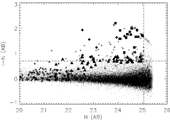
Figure 3.— Plot of emission-line excess objects ($I-N$ vs. $N$) found in the NB816 narrowband filter as a function of object magnitude. Narrow-band magnitudes are given in the AB system (Oke & Gunn, 1983; Oke, 1990) of equivalent visual magnitudes. The distribution of field objects is also shown as a scatter plot. Filled symbols show the properties of spectroscopically identified emission-line objects (triangles are [O II] emitters, diamonds are [O III] emitters, and squares are candidate $z\sim 5.7$ Ly$\alpha$ emitters) and crosses inside open diamonds are candidates which were spectroscopically observed but not identified. An $(I-N)>0.7$ and $N<25.05$ selection criterion (dashed lines) picks out 127 objects which are shown with crosses if they have not been spectroscopically observed. Asterisks mark the positions of known stars.

The high-$z$ objects are also expected to have very red colors because of the effects of the Ly$\alpha$ forest scattering and of the intrinsic Lyman continuum breaks in the galaxies themselves. For a $z\sim 5.7$ object whose Ly$\alpha$ emission is in the narrow band, the scattering in the $R$ band will be a mixture of Ly$\beta$ from the intergalactic medium at $z\sim 5.4$ and Ly$\alpha$ from $z\sim 4.5$. Their combined effects result in a transmission of only about 20% of the light at this wavelength based on measurements of brighter quasars (Songaila 2004, in preparation). This corresponds to an $R-z^{\prime}_{AB}$ break of about 1.8 mags so that we expect the actual $R-z^{\prime}$ colors for the objects to be redder than this value. By contrast we expect that [O II] lines which have the Balmer and 4000 Å breaks between the two bands will have weaker $R-z^{\prime}_{AB}$ breaks of up to about a magnitude, while [O III] or H$\alpha$ lines should have nearly flat continua over the $R-z^{\prime}$ wavelength range. At wavelengths less than about 6000 Å we expect the galaxies to be faint owing to Lyman continuum absorption and that this should result in a $z\sim 5.7$ galaxy being undetected in the $B$ and $V$ bands.

We illustrate this in Figure 4 where we show the $R-z^{\prime}$ color versus the narrow band excess $I-N$ for all the brighter objects with $N_{AB}<23.8$ in the field. Known [O II] and [O III] emitters are marked. At this bright narrowband magnitude cut the color regions populated by stars and foreground galaxies are very well defined, and we can use this to define a region (solid lines) in which $z\sim 5.7$ Lyman alpha galaxies can be unambiguously distinguished from foreground populations. The regions of the [O III] and [O II] emitters can clearly be seen. As expected, the [O III] emitters are nearly flat in $R-z^{\prime}_{AB}$ with typical values of 0.0 to 0.3. These objects can have extremely high equivalent widths, however. By contrast the [O II] emitters have lower equivalent widths, with only a few exceeding $I-N_{AB}\sim 0.7$, but have redder colors. The higher equivalent width [O II] objects in Figure 4 appear to be slighter bluer than the weaker ones, with typical $R-z^{\prime}_{AB}$ colors of just under one. At these magnitudes there are no objects in the field with red enough colors to be a $z\sim 5.7$ emitter with $I-N_{AB}>0.7$.

Figure 4.— Plot of emission-line excess objects ($R-z^{\prime}$ vs. $I-N$) found in the NB816 narrowband filter for a bright $N<23.8$ selection. The distribution of field objects is also shown as a scatter plot. Filled symbols show the properties of spectroscopically identified emission-line objects (triangles are [O II] emitters, diamonds are [O III] emitters, and open diamonds are candidates which were spectroscopically observed but not identified. Plus signs indicate objects which satisfy the $(I-N)>0.7$ condition (shown as the dashed line), but which have not been spectroscopically observed. Asterisks show spectroscopically identified stars. The adopted selection criteria for unambiguous $z\sim 5.7$ Ly$\alpha$ emitters in this color-color plane is shown by the solid lines. This figure may be compared to a similar color plot (Fig. 6) for a faint narrowband selection, $23.8<N<25.05$, which spans the magnitude range of the newly discovered $z\sim 5.7$ Ly$\alpha$ galaxies.

Figure 4 shows that red stars can lie in a simple $I-N_{AB}>0.7$ plus red color break selected sample since at the red end the star track angles into this region. The reason for this is that the narrow band lies between strong stellar absorption features lying in the $I$ band and these strengthen for redder stars through to L types. This results in an apparent excess in the narrow band. This result can be used beneficially in color selection procedures to separate out stars from high-$z$ galaxies or quasars (Kakazu et al. 2004, in preparation) but for the present work we must also eliminate the star track. We have therefore used a slightly higher $I-N_{AB}$ boundary at the reddest $R-z^{\prime}_{AB}$ levels which is illustrated in Figure 4.

The stars can also be distinguished from candidate Ly $\alpha$ emitters on the basis of their $N_{AB}-z^{\prime}$ colors. The location of the star track is shown by the $I-z^{\prime}$ vs $N_{AB}-z^{\prime}$ color-color plot of Fig. 5. The dashed line gives the $I-N_{AB}>0.7$ selection criterion, and the stars and boxes show the track for low-mass stars (including L and T dwarfs) for this filter system. Because the Ly$\alpha$ emission falls within the $I$ band and can be a substantial contributor to the measured broad-band flux, these objects can have blue $I-z^{\prime}$ colors. In general for $I-N_{AB}>0.7$ selected objects the emitters lie at $N_{AB}-z^{\prime}<0.2$ and the stars lie at $N_{AB}-z^{\prime}>0.2$. Because the level of star contamination is low and we wished to avoid eliminating ambiguous cases we did not apply this criterion prior to the spectroscopic observations and chose instead to leave a small number of stars in the candidate sample. We will discuss these objects in the section on the spectroscopy.

Figure 5.— $I-z^{\prime}$ vs. $N-z^{\prime}$ color distribution of spectroscopically identified narrowband excess objects with $I-N>0.7$ (dashed line) compared with the spectroscopically identified stars in the field. Object identifications have been indicated with the usual plot symbols. Squares are Ly$\alpha$ emitters, diamonds are [O III] emitters, triangles are [O II] emitters and asterisks are stars. The distribution of L and T dwarf stars is shown by the small open boxes which are drawn from the literature (Kakazu et al. 2004, in preparation) and lie at redder $N-z^{\prime}$ colors (dotted line) compared to the identified Ly$\alpha$ emitters. Two objects in Table 3 which are spectroscopically unidentified but which are probably stars are marked with open diamonds.

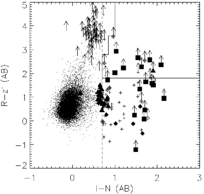
Figure 6.— Color distribution of narrowband excess objects in $R-z^{\prime}$ for the $N>23.8$ and $N<25.05$ sample. These data may be compared with the bright ($N<23.8$) sample color distribution of Fig. 4, where the color tracks of galaxies and stars and the locations of foreground emission-line galaxies may be more clearly seen. Object identifications have been indicated with the plot symbols. Squares are Ly$\alpha$ emitters, triangles are [O II] emitters, diamonds are [O III] emitters, plus signs are $(I-N)>0.7$ (dashed line) objects which were not spectroscopically observed, and asterisks are stars. The adopted selection criteria for unambiguous $z\sim 5.7$ Ly$\alpha$ emitters indicated in Fig. 4 is shown by the solid lines. $R-z^{\prime}$ color breaks for faint objects are generally limited by the $R$ band non-detection sensitivity.

Our final sample of objects was then taken as all objects with $N_{AB}<25.05$ which clearly lay within the designated area of $R-z^{\prime}$, $I-N_{AB}$ color-color space and which were also not detected in $V$ or $B$, together with objects which satisfied the emission line criterion and were not detected at any wavelength shortward of $I$. Their $R-z^{\prime}$ vs. $I-N_{AB}$ color properties are shown in Fig. 6, with object symbols as previously defined. Arrows show 2 $\sigma$ limits on the colors.

Table 3Properties of Candidate Sample

Object	RA(2000)	Dec(2000)	$N(AB)$	$Z(AB)$	$I$	$R$	$V$	$B$	$z$
01	334.220001	0.277625	25.0	28.7	28.6	99.0	99.0	99.0	5.659
02	334.229004	0.093959	23.9	26.5	26.0	99.0	99.0	27.7	5.676
03	334.234985	0.246227	24.5	24.9	26.3	28.3	99.0	99.0	5.660
04	334.273010	0.216856	24.4	25.8	26.1	99.0	99.0	29.4	5.670
05	334.278015	0.206272	24.7	25.2	26.3	28.3	99.0	99.0	5.651
06	334.279999	0.462454	24.6	25.6	26.6	30.4	99.0	27.9	$\cdots$
07	334.291992	0.211263	24.6	24.5	25.6	99.0	99.0	31.4	5.626
08	334.308014	0.316606	24.9	24.5	25.6	26.9	99.0	99.0	$\cdots$
09	334.317993	0.223775	24.6	25.2	25.8	28.3	99.0	29.3	5.645
10	334.320007	0.359441	25.0	25.5	25.8	99.0	99.0	99.0	$\cdots$
11	334.337006	0.335259	24.5	27.0	26.2	27.8	27.0	27.2	5.669
12	334.337006	0.293762	24.1	24.8	25.6	99.0	99.0	99.0	5.667
13	334.351990	0.197130	24.7	27.3	27.9	28.4	26.9	99.0	obs
14	334.369995	0.321620	24.2	25.0	25.2	27.1	28.3	28.2	5.641
15	334.381989	0.160189	24.5	25.9	26.5	28.6	99.0	27.9	5.684
16	334.388000	0.371196	24.3	26.1	25.9	28.0	26.6	99.0	5.653
17	334.389008	0.390323	24.6	23.9	25.5	27.6	99.0	26.8	star?
18	334.415985	0.307220	24.8	26.6	26.4	28.4	28.1	26.7	5.723
19	334.420013	0.404125	24.9	25.7	25.7	28.8	27.8	99.0	5.633
20	334.420013	0.118385	24.5	25.4	26.6	99.0	29.2	99.0	1.173
21	334.425995	0.128724	24.4	24.9	26.1	99.0	28.3	99.0	5.687
22	334.492004	0.228247	24.9	25.0	25.7	27.9	99.0	99.0	0.492?
23	334.509003	0.242099	24.1	25.9	25.9	99.0	99.0	99.0	5.673
24	334.519012	0.239439	24.8	27.4	28.7	99.0	99.0	99.0	5.680
25	334.548004	0.083544	23.8	25.1	25.9	28.1	99.0	28.4	5.709
26	334.556000	0.095670	25.0	27.2	26.9	99.0	99.0	99.0	5.682

Note. — Magnitudes are measured in 3^′′ diameter apertures. An entry of ‘99’ indicates that no excess flux was measured.

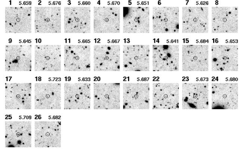
Figure 7.— Narrowband 8150/120 Å images of the 26 emission-line candidates selected in Table 3. Each field is 30^′′ on a side. A 2^′′ radius circle identifies each candidate, which is labeled by object number and redshift (for confirmed high-$z$ galaxies). This figure may be contrasted with the corresponding $R$-band images of Fig. 8.

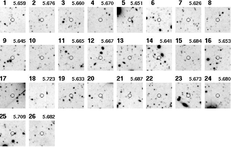
Figure 8.— $R$-band images of the selected emission-line candidates shown in Fig. 7. A 2^′′ radius circle indicates the candidate’s location in each $30^{\prime\prime}\times 30^{\prime\prime}$ field. Candidates are labeled by object number and redshift (for confirmed high-$z$ galaxies) from Table 3. Absorption due to the Lyman alpha forest should suppress $R$-band light from redshift $z\sim 5.7$ galaxies.

This final candidate sample contains 26 objects. Tabulated coordinates, multi-color magnitudes, and redshifts (where measured) for these objects are summarized in Table 3. Thumbnail finding charts in the narrowband (Fig. 7) and $R$-band (Fig. 8) are shown, with the objects encircled. Each thumbnail is 30^′′ on a side, with the circles $2^{\prime\prime}$ in radius.

4. Spectroscopic classification

Twenty-two of the 26 objects in the candidate list were observed with DEIMOS with exposure times ranging from 1.5 to 4.5 hours. A randomly chosen sample of 21 additional objects with $(I-N)>0.7$ which did not satisfy the color selection was also observed with the choice of objects in this case being determined by the mask configurations. One additional object in the candidate list which had been previously observed with LRIS was not included in the DEIMOS masks. The DEIMOS masks were filled with color selected and magnitude selected samples which will be described elsewhere and contained just over 900 objects.

All of the spectra (emission line and field objects) were spectroscopically classified without reference to their narrow band strengths and color properties. As can be seen from Fig. 2 at the DEIMOS resolution [O II] and [O III] lines are easily distinguished based on their doublet structure, while H$\alpha$ emitters can usually be picked out on the basis of the [N II] or [S II] doublets or using the H$\beta$, [O III] complex. Only a small number of emission line objects show single broad asymmetric lines of the type illustrated in Fig. 2 and these were classified as Ly$\alpha$ emitters. Where there was uncertainty in the classification the object was marked as observed but unidentified. Where an object was observed multiple times each spectrum was measured individually. However, there was no disagreement among identifications and in the final compilation these spectra were averaged.

Figure 9.— Extracted DEIMOS spectra of single-line emission line objects with asymmetric profiles in the candidate sample. Spectra are labeled with the assigned object number and redshift given in Table 3. The bottommost plots show the positions of strong nightsky lines for comparison with subtraction residuals (e.g., objects 18, 23, 24, 25, 12, 4, and 2).

Figure 10.— Spectra of emission line objects with the [O II] doublet signature. Candidate object 20, from Table 3 is identified as an [O II] emitter at redshift $z=1.172$. The remaining 8 spectra show galaxies selected according to [O II] emission excess within the narrowband filter. As for Fig. 9, the bottom spectrum shows the positions of the strong nightsky lines which may give rise to subtraction residuals.

Figure 11.— Spectra of emission line objects with the [O III] doublet signature. As in Fig. 9, the bottom spectrum shows the positions of the strong nightsky lines which may give rise to subtraction residuals.

The redshift identifications of the high $z$ candidate list are summarized in Table 3. Of the 22 DEIMOS observed objects 18 were identified as Lyman alpha emitters, as was the LRIS observed object. One object was classified as an [O II] emitter and three could not be clearly identified. The spectra of the identified $(N-I)>0.7$ objects are shown in Figures 9, 10, and 11. One of the unidentified objects has a weak continuum spectra which probably corresponds to a star and lies in the area of $z^{\prime}-N$, $I-N$ color-color space consistent with this interpretation as does one of the unobserved objects (17 and 8 respectively). One object (21) has a strong red emission line which is symmetric and narrow and which, if it is H$\alpha$, places the object at redshift $z=0.492$. There is a weak feature at the [O III] $\lambda$5007 emission position which could be consistent with this interpretation but, irrespective, this object is clearly not a $z\sim 5.7$ Lyman alpha emitter. Finally, a retrospective analysis of the [O II] emission line classified object (20) suggests it is ambiguous whether it should have been classified in this way since the [O II] lines are slightly displaced from the correct positions. It is possible this is actually a Lyman alpha emitter. As we show in Fig. 12 if this object is an [O II] emitter its colors are extremely anomalous.

Figure 12.— Color-color plots in $R-z^{\prime}$ vs. $I-N$ of [O II] emitters (triangles) and [O III] emitters (diamonds). [O II] emission-line galaxies display a shallow continuum break in ($R-z^{\prime}$) of about 1 magnitude. The range of emission-line excess ($I-N$) reflects the cut-off of selection criteria at the low excess end, but is generally modest. The [O III] emitters in the narrow-band filter can display stronger observed-frame excess emission, reflected in the wider range of emission excess in ($I-N$). The [O III] galaxies have generally flat spectra ($R-z^{\prime}$) $\sim 0$, but there is a bluing trend seen in the ($R-z^{\prime}$) colors for galaxies with very strong [O III] emission lines. The one object classified as an [O II] emitter (object #20) in the candidate sample lies in the upper right corner of the left hand panel.

For the remainder of the work we will focus on the 19 spectroscopic Ly$\alpha$ emitters recognizing that a further 4 objects could fall in the sample. This small level of incompleteness does not affect the discussion in any statistically significant way.

5. Results and Discussion

5.1. Spatial and spectral distributions

In Figure 13 we show the distribution of the 19 Lyman alpha redshifts compared with the nominal transmission profile of the filter shown by the dotted line. All but one of the 19 objects lie below the redshift corresponding to the $8150\AA$ central wavelength of the filter. The [O III] emitters also lie in the lower half of the filter and taken together these results could suggest that the true on-telescope center of the filter is shorter than the measured value. However, both could be the result of structuring at the respective redshifts. Even if we shift the filter center 25 Å blueward to match the [O III] data (dashed line) 16 of the 19 Ly$\alpha$ emitters still lie in the lower half of the filter. The probability of seeing such a biased result is only 0.0003 while with the laboratory traced filter profile the probability would drop to $2\times 10^{-6}$. It appears that the sample is extremely structured in velocity space.

Figure 13.— The redshift distribution of Ly$\alpha$ emission galaxies compared to the transmission profile of the narrow band filter (dotted line). Nearly all of the objects lie at the low redshift end of the selection, This result remains true even if we shift the filter center $25$ Å to the blue (dashed line).

Figure 14.— The spatial distribution of the 19 Ly$\alpha$ emission galaxies is shown by the large solid ($z<5.687$) and open ($z>5.687$) boxes. The remaining objects in the candidate list are shown as crosses for unidentified objects, asterisks for possible stars, and the small box for the possibly misclassified [O II] emitter which, if it were a Lyman alpha emitter, would lie in the lower redshift interval. Many of the low $z$ objects lie in the large diagonal filament which runs across the field. Most of the objects in this region lie in the more restricted redshift interval $z=5.632-5.672$. Objects lying in this redshift region are enclosed in larger open boxes.

The objects lying in the lower redshift interval also appear to be clustered in space, with many of them lying in a long elongated filament running diagonally across the field (Figure 14). All of the objects between $z=5.632-5.672$ lie in this region.

We postpone a more detailed discussion of the correlation function properties until the analysis of the multi field sample but the present results emphasize that single fields may vary considerably even with areas as large as the present ones and that many independent fields are required to average out these systematic effects.

5.2. Line Shapes

Figure 15.— The stacked Ly$\alpha$ emission line profile of the eighteen new $z\sim 5.7$ galaxies reported in this paper. Individual extracted spectra were normalized to their maximum value, converted to their rest-frame wavelength scale using the redshift corresponding to their peak flux, and co-added. The instrumental profile as determined from neighboring resolved nightsky lines is overplotted on the peak for comparison. The asymmetric profile can be clearly seen.

As can be seen from Figure 9 the Ly$\alpha$ shapes are remarkably uniform, consisting of a slightly peaked profile and a trailing red wing. In Figure 15 we show the stacked profiles of the 18 Ly$\alpha$ emitters with DEIMOS spectra compared with the resolution element of the instrument, which clearly illustrates this point, but individual profiles are also generally similar in shape and width. This type of profile is a simple outcome of the blue truncation of the spectrum as is illustrated in Figure 16 where we show a simple model where the intrinsic line is modeled as a Gaussian and then is truncated below the object redshift by the Lyman alpha scattering of the IGM. When this profile is convolved through the instrument resolution it produces an observed spectrum almost identical to that observed as is shown in the lower panel of the figure.

Figure 16.— A simple model profile for the Ly$\alpha$ emission feature in Fig. 15. The top profile shows a Gaussian emission-line profile with Doppler width $\sigma=200$ km s^-1 with the blue half of the line (dashed curve) absorbed by the foreground Ly$\alpha$ forest. When this is convolved with the instrumental profile of the spectrograph, the resulting profile (dashed curve) shows a good fit to the observed stacked Ly$\alpha$ profile (solid curve) in the bottom half of the figure.

The required width of the intrinsic line which matches the observed stacked spectrum corresponds to a $\sigma$ of 200 km s^-1 and this value also produces a reasonable fit to nearly all the individual line profiles. This is much wider than would be expected from the velocity dispersions of the parent galaxies at this redshift and almost certainly represents velocity broadening of the Ly$\alpha$ during the escape from the galaxy. Given the complexity of this process there is probably relatively little useful information in the widths. The truncation also results in the measured redshifts, which were set to the peak of the line, being about a 100 km s^-1 redward of the true redshift,

5.3. Equivalent Widths

Since the narrow band lies almost precisely in the center of the $I$ band the truncation effect reduces the $I$ band flux and the narrow band flux in very similar amounts and we shall assume that the equivalent widths (EWs) of the lines do not need to be corrected for this effect. (This approximation does depend on the IGM scattering not extending substantially redward of the line center which could be incorrect.) Because the filter is not rectangular in shape we do need to allow for the filter profile in computing the EWs.

The simplest approach is to compute the equivalent widths based on the $I$ and $N$ magnitudes. Defining the quantity

$$R=10^{-0.4*(N-I)}$$

the observed frame equivalent width becomes

$$EW=\left[{R-1}\over{\displaystyle{\phi-{R\over{\Delta\lambda}}}}\right]$$

where $\phi$ is the narrow band filter response normalized such that the integral over wavelength is unity and $\Delta\lambda$ is the effective width of the $I$ filter, which is approximately 1400 Å. The narrow band filter is often assumed to be rectangular in which case $\phi$ becomes $1/\Delta\lambda$ where $\Delta\lambda$ is the width of the narrow band (e.g., Rhoads & Malhotra, 2002) but as can be seen from Figure 13 this is not a very good approximation in the present case.

For very high equivalent width objects such as the Lyman alpha emitters the denominator in this equation becomes uncertain unless the broad band data is very deep and this can result in a very large scatter in the measured equivalent widths. Therefore in order to check the result we also computed the equivalent widths by extrapolating from the $z^{\prime}$ observations assuming that these provide a better measure of the true continuum flux. We assumed in this case that the spectral energy distribution was flat in frequency space giving the formula

$$EW=\left[{2\times{\rm Norm}\times(R_{2}-1)}\over{\displaystyle{\phi}}\right]$$

where

$$R_{2}=10^{-0.4*(z^{\prime}-N)}$$

and Norm is the square of the wavelength ratio of the center of the $z^{\prime}$ filter over that of the narrow band. In order to avoid uncertainties from the exact wavelength center of the filter we restrict ourselves to wavelengths where the nominal filter response is more than 0.67 of the peak.

The rest frame equivalent widths calculated with both methods generally agree well with each other though there are significant differences in a small number of individual cases. The distribution based on the extrapolated fluxes is shown in Fig. 17. In contrast to the results of Malhotra & Rhoads (2002) most of the rest frame equivalent widths have values less than 240 Å, which can be understood in terms of galaxies with Salpeter initial mass functions. (See Malhotra and Rhoads for an extensive discussion of this issue.) As discussed in the previous paragraph, the equivalent width determination is very sensitive to the depth of the continuum band exposures, and the difference between the present results and those of Malhotra & Rhoads (2002) may arise from the deeper continuum exposures used here. Only four of the objects have poorly defined rest frame equivalent widths and are shown at nominal values of 240 Å in the figure but even these objects could well lie at lower values based on the uncertainties in the determination. The overall distribution of Fig. 17 is quite similar to the distributions measured at lower redshifts (e.g. Figure 21 of Fujita et al. (2003) which summarizes these measurements.)

Figure 17.— Rest frame equivalent width distribution for the 15 Lyman alpha emitters lying in the redshift range where the filter profile lies above 0.67 times its maximum value.

Figure 18.— The luminosity function based on the Ly$\alpha$ emission line for the $z\sim 5.7$ emitters (filled squares) compared to the emission line luminosity function at $z\sim 3.4$ (open squares). The vertical dashed line indicates the limits of the sample, which does not yet reach the flat part of the $z\sim 5.7$ luminosity function.

5.4. Lyman alpha Luminosity Function

Because of the high observed frame equivalent widths the Ly$\alpha$ fluxes are insensitive to the continuum determination. However, they do depend on the filter response at the emission line wavelength so we have again restricted ourselves to redshifts where the nominal filter response is greater than 67% of the peak value.

Because the volume is simply defined by the selected redshift range the luminosity function may be obtained by dividing the number of objects in each luminosity bin by the volume. The calculated Ly$\alpha$ luminosity function is shown in Figure 18, where we compare it with the $z=3$ luminosity function computed from the results of Hu et al. (1998). The observations of Kudritzki et al. (2000) give a similar value at this redshift. The present function samples generally higher luminosities than the $z=3$ samples but is broadly consistent in number density at the lowest luminosities. It lies slightly above the Fujita et al. (2003) values at similar luminosities, but this probably reflects the higher equivalent width selection that was used in that work.

Figure 19.— The luminosity function of the UV continuum of $z\sim 5.7$ emitters compared with the Steidel et al. 1999 UV luminosity functions at redshifts 3 (diamonds) and 4 (triangles). Measured points from the Ly$\alpha$ emitters are shown as solid boxes; the open boxes show assumed values if emitters pick out 20% of the LBG sample as Steidel et al. (2000) find to be the case at $z\sim 3$.

5.5. Continuum Luminosity Function

We may also view the Lyman alpha selection as picking out that subset of the Lyman break galaxies (LBGs) at this redshifts which have strong line emission. While some of the objects are very faint in the $z^{\prime}$ band, which corresponds to a rest frame of about $1400$ Å, most (16 of the 19) have well measured $z^{\prime}$ magnitudes lying in the range from 24 to 27. These magnitudes correspond to absolute continuum magnitudes at $1450$ Å which are very similar to the typical LBG at $z=3-4$. The use of continuum magnitudes to estimate the star formation rates avoids the extremely complex problems of the Lyman alpha escape process and the uncertainties in the correction of the Lyman alpha fluxes for intergalactic scattering which are present in the determination of the Ly$\alpha$ luminosity function.

Figure 19 shows the continuum luminosity function derived from the distribution of the $z^{\prime}$ magnitudes. Once again we have restricted ourselves to objects lying in the higher transmission region in the filter. The solid boxes show the measured values with 1 $\sigma$ Poisson uncertainties based on the number of objects in the bin. There are no objects with absolute magnitudes brighter than $-22$ and for the final data point we show a 1 $\sigma$ upper limit. No correction has been applied for dust. Figure 19 also shows the raw (dust uncorrected) UV luminosity function for Lyman break selected galaxies at redshifts $z\sim 3$ (open diamonds) and $z\sim 4$ (open triangles) (Steidel et al., 1999, 2000). At these redshifts Steidel et al. (2000) found the Lyman alpha selection picks out about $20\%$ of the Lyman break galaxies. The open squares show the values which would be obtained for the LBG luminosity function at $z=5.7$ if the Lyman alpha selected fraction were similar to that at the lower redshift. It matches extremely closely to the lower redshift luminosity functions. The Ly$\alpha$ selected fraction at these redshifts could be larger, and comparison with the color-selected samples of Stanway et al. (2003) would be consistent with this interpretation.

Once again, recognizing the systemic uncertainties in a single field observation and the uncertainties involved in the Ly$\alpha$ selected fraction, we postpone a more detailed discussion to a subsequent paper. However, it is clear already from Figure 19 that star formation rates at $z=5.7$ are roughly similar to those at lower redshift and there is no rapid decline in the star formation rates at these redshifts.

6. Conclusions

We may summarize the major conclusions of the paper as follows.

1) Combined emission line and color break techniques provide an extremely efficient method of selecting objects at $z=5.7$. Selection criteria of $(N-I)>0.7$, $(R-z^{\prime})>1.8$ and $(N-z^{\prime})<0.2$ pick out 24 objects in the field. At least 19 of these are spectroscopically confirmed as Lyman alpha emitters at this redshift. Only one or at most two of the sample selected in this way are lower redshift interlopers. The accuracy is sufficiently good to allow use of color selected samples without the necessity of spectroscopic followup for many purposes.

2) Even on scales as large as the present 26^′ field the distribution of objects is highly structured in both the spectral and spatial dimensions. Individual fields could easily show factors of several variation in the number density of objects selected in a 100 Å bandpass and a substantial number of fields need to be observed to average out these effects.

3) The properties of the Lyman alpha selected galaxies are quite similar to those observed at $z\approx 3$.

4) Star formation rates at $z=5.7$ are roughly similar to those at $z=3$ and $z=4$ though there are very substantial uncertainties in this estimate.

References

- Ajiki et al. (2002) Ajiki, M. et al. 2002. ApJ, 576, L25, astro-ph/0207303
- Ajiki et al. (2003) Ajiki, M. et al. 2003. AJ, 126, 2091, astro-ph/0307325
- Barger et al. (2002) Barger, A. J., Cowie, L. L., Brandt, W. N., Capak, P., Garmire, G. P., Hornschemeier, A. E., Steffen, A. T., & Wehner, E. H. 2002, AJ, 124, 1839, astro-ph/0206370
- Bouwens et al. (2003) Bouwens, R. J. et al. 2003, ApJ, 595, 589, astro-ph/0306215
- Bunker et al. (2003) Bunker, A. J., Stanway, E. R., Ellis, R. S., McMahon, R. G., & McCarthy, P. J. 2003, MNRAS, 342, L47, astro-ph/0302401
- Capak et al. (2004) Capak, P. et al. 2004, AJ, in press (http://www.ifa.hawaii.edu/capak/hdf/)
- Cowie & Hu (1998) Cowie, L. L., & Hu, E. M. 1998, AJ, 115, 1319, astro-ph/9801003
- Cowie et al. (1994) Cowie, L. L., Gardner, J. P., Hu, E. M., Songaila, A., Hodapp, K.-W., & Wainscoat, R. J. 1994, ApJ, 114
- Cuby et al. (2003) Cuby, J. G., LeFèvre, O., McCracken, H, Cuillandre, J.-C., Magnier, E., & Meneux, B. 2003, A&A, 405, L19, astro-ph/0303646
- Cuillandre et al. (2000) Cuillandre, J.-C., Luppino, G. A, Starr, B. M., & Isani, S. 2000, Proc. SPIE, 4008, 1010
- Dawson et al. (2002) Dawson, S., Spinrad, H., Stern, H., Dey, A., van Breugel, W., de Vries, W., & Reuland, M. 2002, astro-ph/0201194
- Dey et al. (1998) Dey, A., Spinrad, H., Stern, D., Graham, J. R., & Chaffee, F. H. 1998, ApJ, 498, L93, astro-ph/9803137
- Dickinson et al. (2003) Dickinson, M. et al. 2003, ApJ, in press, astro-ph/0309070
- Ellis et al. (2001) Ellis, R., Santos, M. R., Kneib, J., & Kuijken, K. 2001, ApJ, 560, L119, astro-ph/0109249
- Faber et al. (2003) Faber, S. M. et al. 2003, Proc. SPIE, 4841, 1657
- Fan et al. (2001) Fan, X. et al. 2001, AJ, 122, 2833, astro-ph/0108063
- Fan et al. (2003) Fan, X. et al. 2003, AJ, 125, 1649, astro-ph/0301135
- Fujita et al. (2003) Fujita, S. S. et al. 2003, AJ, 125, 13, astro-ph/0210055
- Hu et al. (1998) Hu, E. M., Cowie, L. L., & McMahon, R. G. 1998, ApJ, 502, L99, astro-ph/9801003
- Hu et al. (1999) Hu, E. M., Cowie, L. L., & McMahon, R. G. 1999, in ASP Conf. Ser. 193, The Hy Redshift Universe, ed. A. J. Bunker & W. J. M. van Breugel (San Francisco: ASP), 554, astro-ph/9911477
- Hu et al. (1999) Hu, E. M., McMahon, R. G., & Cowie, L. L. 1999, ApJ, 522, L9, astro-ph/9907079
- Hu et al. (2002) Hu, E. M., Cowie, L. L, McMahon, R. G., Capak, P., Iwamuro, F., Kneib, J.-P., Maihara, T., & Motohara, K. 2002, ApJ, 568, L75 (erratum 576, L99), astro-ph/0203091
- Iwata et al. (2003) Iwata, I. et al. 2003, PASJ, 55, 415, astro-ph/0301084
- Kodaira et al. (2003) Kodaira, K. et al. 2003, PASJ, 55, L17, astro-ph/0301096
- Kudritzki et al. (2000) Kudritzki, R.-P. et al. 2000, ApJ, 536, 19, astro-ph/0001156
- Landolt (1992) Landolt, A. U. 1992, AJ, 104, 340
- Lehnert & Bremer (2003) Lehnert, M. D., & Bremer, M. 2003, ApJ, 593, 630, astro-ph/0212431
- Maier et al. (2003) Maier, C., Meisenheimer, K., Thommes, E., Hippelein, H., Röser, H. J., Fried, J., von Kuhlmann, B., Phleps, S., & Wolf, C. 2003 A&A, 402, 79, astro-ph/0302113
- Malhotra & Rhoads (2002) Malhotra, S., & Rhoads, J. E. 2002, ApJ, 565, L71, astro-ph/0111126
- Miyazaki et al. (2002) Miyazaki, S., et al. 2002, PASJ, 54, 833
- Oke (1990) Oke, J. B. 1990, AJ, 99, 1621
- Oke & Gunn (1983) Oke, J. B. & Gunn, J. E. 1983, ApJ, 266, 713
- Oke et al. (1995) Oke, J. B. et al. 1995, PASP, 107, 375
- Ouchi et al. (2003) Ouchi, M. et al. 2003, ApJ, 582, 60, astro-ph/0202204
- Rhoads & Malhotra (2002) Rhoads, J. E. & Malhotra, S. 2002, ApJ, 565, 71, astro-ph/0110280
- Rhoads et al. (2003) Rhoads, J. E. et al. 2003, AJ, 125, 1006, astro-ph/0209544
- Shimasaku et al. (2003) Shimasaku, K. et al. 2003, ApJ, 586, L111, astro-ph/0302466
- Songaila & Cowie (2002) Songaila, A. & Cowie, L. L. 2002, AJ, 123, 2183, astro-ph/0202165
- Stanway et al. (2003) Stanway, E. R., Bunker, A. J., & McMahon, R. G. 2003, MNRAS, 342, 439, astro-ph/0302212
- Steidel et al. (1999) Steidel, C. C., Adelberger, K. L., Giavalisco, M., Dickinson, M., & Pettini, M. 1999, ApJ, 519, 1, astro-ph/9811399
- Steidel et al. (2000) Steidel, C. C., Adelberger, K. L., Shapley, A. E., Pettini, M., Dickinson, M., & Giavalisco, M. 2000, ApJ, 532, 170, astro-ph/9910144
- Steidel et al. (2001) Steidel, C. C., Pettini, M., & Adelberger, K. L. 2001, ApJ, 546, 665, astro-ph/0008283
- Stern & Spinrad (1999) Stern, D., & Spinrad, H. 1999, PASP, 111, 1475, astro-ph/9912082
- Taniguchi et al. (2003) Taniguchi, Y. et al. 2003, ApJ, 585, L97, astro-ph/0301635
- Turnshek et al. (1990) Turnshek, D. A., Bohlin, R. C., Williamson II, R. L., Lupie, O. L., Koornneef, J., & Morgan, D.H. 1990, AJ, 99, 1243
- van Breugel et al. (1999) van Breugel, W. J. M., de Breuck, C., Stanford, S. A., Stern, D., Röttgering, H., & Miley, G. 1999, ApJ, 518, L61, astro-ph/9904272
- Weymann et al. (1998) Weymann, R. J., Stern, D., Bunker, A., Spinrad, H., Chaffee, F. H., Thompson, R. I., & Storrie-Lombardi, L. J. 1998, ApJ, 505, L95, astro-ph/9807208
- SuprimeCam filters (2003) http://www.naoj.org/Observing/Instruments/SCam/sensitivity.html Filter response curve web page referenced in §2.1