The Chemical Composition Contrast between M3 and M13 Revisited: New Abundances for 28 Giant Stars in M3.

Abstract

We report new chemical abundances of 23 bright red giant members of the globular cluster M3, based on high-resolution (R $\sim$ 45000) spectra obtained with the Keck I telescope. The observations, which involve the use of multislits in the HIRES Keck I spectrograph, are described in detail.

Combining these data with a previously-reported small sample of M3 giants obtained with the Lick 3m telescope, we compare metallicities and [X/Fe] ratios for 28 M3 giants with a 35-star sample in the similar-metallicity cluster M13, and with Galactic halo field stars having [Fe/H] $<$ –1. For elements having atomic number A $\geq$ A(Si), we derive little difference in [X/Fe] ratios in the M3, M13 or halo field samples.

All three groups exhibit C depletion with advancing evolutionary state beginning at the level of the red giant branch “bump”, but the overall depletion of about 0.7 to 0.9 dex seen in the clusters is larger than that associated with the field stars. The behaviors of O, Na, Mg and Al are distinctively different among the three stellar samples. Field halo giants and subdwarfs have a positive correlation of Na with Mg, as predicted from explosive or hydrostatic carbon burning in Type II supernova sites. Both M3 and M13 show evidence of high-temperature proton capture synthesis from the ON, NeNa, and MgAl cycles, while there is no evidence for such synthesis among halo field stars. But the degree of such extreme proton-capture synthesis in M3 is smaller than it is in M13: the M3 giants exhibit only modest deficiencies of O and corresponding enhancements of Na, less extreme overabundances of Al, fewer stars with low Mg and correspondingly high Na, and no indication that O depletions are a function of advancing evolutionary state as has been claimed for M13.

We have also considered NGC 6752, for which Mg isotopic abundances have been reported by Yong et al. (2003). Giants in NGC 6752 and M13 satisfy the same anticorrelation of O abundances with the ratio (²⁵Mg+²⁶Mg)/²⁴Mg, which measures the relative contribution of rare to abundant isotopes of Mg. This points to a scenario in which these abundance ratios arose in the ejected material of 3-6 solar mass cluster stars, material that was then used to form the atmospheres of the presently evolving low-mass cluster stars. It also suggests that the low oxygen abundance seen among the most evolved M13 giants arose in hot-bottom O to N processing in these same intermediate-mass cluster stars. Thus mixing is required by the dependence of some abundance ratios on luminosity, but an earlier nucleosynthesis process in a hotter environment than giants or main-sequence stars is required by the variations previously seen in stars near the main sequence. The nature and the site of the earlier process is constrained but not pinpointed by the observed Mg isotopic ratio.

1 INTRODUCTION

Thirty years have elapsed since the initial discovery (Osborn 1971) of CN variations among giants in an otherwise mono-metallic globular cluster. A flood of evidence has now accumulated indicating that several light elements, not only carbon and nitrogen, but also oxygen, sodium and aluminum have large and often correlated abundance variations among the giants of individual clusters (see reviews by Kraft 1994, Briley et al. 1994, Wallerstein et al. 1997, DaCosta 1998). The range of variation in some of these elements often exceeds an order of magnitude, far more than expected from conventional “first dredge-up” predictions (see Iben & Renzini 1984). It is clear that the surface chemical compositions of most cluster giants are reflections of the products of multiple proton-capture chains (Denissenkov & Denissenkova 1990; Cavallo et al. 1996; Langer, Hoffman & Zaidins 1997; Denissenkov et al. 1998) which involve conversion not only of C to N, but also O to N, Ne to Na and Mg to Al.

Less well understood is the site (or indeed sites) in which proton-capture syntheses actually take place. Two possible scenarios have been invoked. In the first, the “primordial” picture, the variations are a result of pre-existing syntheses which made contributions to the gas out of which the presently observable low-mass stars were assembled. This approach has two subcases: (1) the stars formed from gas already possessing these variations at the epoch of cluster formation, a truly “primordial” picture, or (2) the presently observed low-mass stars were “polluted” by the accretion of processed material ejected by intermediate-mass (3-6 $M_{\odot}$) stars in their late evolutionary stages (Cottrell & DaCosta 198l, Cannon et al. 1998, Ventura et al. 2001, Yong et al. 2003). In either subcase, variations in C, N, O, Na and Al abundances should exist among main-sequence, or near main-sequence turnoff, stars in clusters.

Observational examples supporting this picture are readily forthcoming. For instance, CN bimodality persists among giants well down onto the subgiant branch in several clusters (e.g., Hesser, Hartwick, & McClure 1977, Smith & Norris 1982, Norris & Smith 1984, Cannon et al. 1998, Smith 2002a,b). C and N abundance inhomogeneities have been observed among subgiant and even main-sequence stars in M5 and NGC 6752 (Suntzeff & Smith 1991, Cohen et al. 2002) and M71 (Cohen 1999). Moreover, variations involving other light elements among such relatively unevolved stars have recently come to light, e.g., the correlation of CN band strengths and Na in main sequence stars of 47 Tuc (Briley et al. 1996), and the anticorrelation of O and Na as well as Al and Mg among main-sequence stars of NGC 6752 (Gratton et al. 2001). O and Na also appear to be anticorrelated among subgiants in M71 (Ramirez & Cohen 2002). Evidence of proton-capture synthesis of Ne into Na and Mg into Al has been found among a small sample of turnoff stars in M92 (King et al. 1998). Large ranges in Na in the case of M5 have been found to persist all the way from the giants to the main sequence (Ramirez & Cohen 2003), and a substantial range in C abundance has been found among main-sequence stars in M13 (Briley et al. 2003). Evidence favoring a primordial source for the variations among these light elements therefore seems well established.

But there is also evidence that the stars we presently observe reshuffle the abundances of many light elements as a result of deep mixing during the ascent of the red giant branch. Material of the stellar envelope is exposed to CN, ON, and in some cases NeNa and possibly even MgAl cycling as it is circulated through regions near or even in the CNO-burning shell of an evolving low-mass, metal-poor star. Among field metal-poor ([Fe/H] $\lesssim$ –1.0) halo stars, Gratton et al. (2000) found a progressive decrease in total C and ${\rm{}^{12}C/^{13}C}$ ratios, with corresponding enhancement of N, as stars evolve up the first giant branch. These observed abundance changes far exceed those predicted from conventional evolutionary models. Among globular cluster giants having [Fe/H] $<$ –1.0, these changes in C and N are even more marked (Langer et al. 1986, Bellman et al. 2001, Trefzger et al. 1983, Briley et al. 1990, Briley et al. 2003) and contrary to the case of field stars, often involve also the ON cycle, so that many cluster giants exhibit depletion of O (Pilachowski 1988, Kraft et al. 1997, Sneden et al. 1997 and references therein) and corresponding enhancement of N. At the same time, in many clusters (e.g., NGC 288, NGC 362, M5, M10, M13, M15) there is an O versus Na anticorrelation, explicable as evidence of NeNa cycling in a region experiencing ON cycling (Langer & Hoffman 1995, Cavallo et al. 1996).

It is not known if the O versus Na anticorrelation is a result of primordial events or a result of deep mixing in the giants we observe. Even more controversial is the origin of the correlation between Al and Na observed among giants in several clusters (Shetrone 1996), since CNO-burning shell temperatures in low-mass, metal-poor red giants do not reach temperatures high enough to permit significant operation of the ²⁴Mg/²⁷Al cycle (Cavallo et al. 1998, Powell 1999, Langer et al. 1997). Shetrone also discovered that the M13 giants of lowest oxygen abundance had anomalously high ratios of (²⁵Mg+²⁶Mg)/²⁴Mg, and a similar result has recently been found in a large sample of giants in NGC 6752 (Yong et al. 2003). Such overabundances of the lesser isotopes of Mg can readily be produced in the evolution of low-metallicity 3 to 6 solar mass AGB stars (Siess et al. 2002), and this strongly suggests that a pollution scenario is in operation. However, the possibility of enhancement of ²⁷Al through proton-captures on ^25,26Mg, operating in a region favorable to NeNa cycling, seems possible in the case of giants in M4 (Ivans et al. 1999). Could such a process also be in operation in M13 and in NGC 6752? Finally, as Cavallo & Nagar (2000) have most recently emphasized (see also Pilachowski et al. 1996, Kraft et al. 1997), the mean Al and Na abundances of M13 giants sharply increase in the last 0.4 mag before the red giant tip. This is hard to understand unless it is the result of deep mixing which brings up the ashes of ²²Ne to ²³Na and ²⁵Mg or ²⁶Mg to ²⁷Al processing in the low-mass giants we presently see. Finally, in indirect support of at least a modest degree of deep mixing is the finding that although main-sequence stars in M13 exhibit a wide range in [C/Fe] ratios, many of which have [C/Fe] well below –0.3 (Briley et al. 2003), the mean [C/Fe] ratio is much lower among giants than dwarfs. It is also true that seven out of 30 M13 giants have [O/Fe] $<$ –0.4 (Kraft et al. 1997), an additional result that is hard to understand on a primordial “pollution” scenario.

A growing consensus emerges that most clusters have stars whose abundance ratios reflect primordial variations, but that these variations are further modified by deep mixing (see, e.g., Briley et al. 1994, Cavallo & Nagar 2000, Briley et al. 2003) as stars evolve up the giant branch. Of special interest is the contention that deep mixing may also play a role as a driver of the so-called “second parameter” effect (Sweigart 1997) in which clusters of closely the same metallicity may nevertheless have quite different horizontal branch morphologies. Critical pairs of clusters exhibiting these differences, for example, are M3 versus M13 and NGC 362 versus NGC 288. Many investigators have argued, based on the study of cluster color-magnitude diagrams, that age is the most likely driver of the second parameter (e.g., Buonanno et al. 1994, Sarajedini et al. 1997, Rey et al. 2001). Others have argued that in at least some of these pairs, particularly M3/M13, the age difference inferred from the relative location of the cluster turnoff luminosity is too small to account for the difference in HB morphology (Stetson et al. 1996, Johnson & Bolte 1998).

Mixing, if it is deep enough to penetrate the hydrogen burning shell, will no doubt increase the He/H ratio in the convective envelopes of the red giant progenitors, so the resulting HB branch descendants are likely to be bluer than would be the case in the absence of deep mixing (Sweigart 1997, Kraft et al. 1998). Since deep mixing appears to be present to a significant degree among M13 giants close to the tip of the first giant branch (Kraft et al. 1997, Cavallo & Nagar 2000), we would expect M13 to possess a very blue HB, and indeed it does in comparison with M3. At the same time, evolved M3 giants show a much smaller degree of deep mixing than do comparable giants in M13 (Kraft et al. 1992, Cavallo & Nagar). However, owing to the fact that M3 is considerably farther from the Sun than is M13, the stars are fainter and less amenable to abundance analysis at high spectral resolution. Thus the published M3 high resolution sample is much smaller than is the case for M13 (10 versus 35). Would more evidence of deep mixing be found in M3, if a larger sample of giant star spectra could be obtained? In addition, Na abundances based on lower resolution spectra are available for 95 additional M13 giants, and of these Mg abundances have been derived for 74 (Pilachowski et al. 1996).

In this paper, we examine more fully the [X/Fe] ratios in M3 based on high resolution analysis of 28 M3 giants. We confirm the tentative earlier result that the Na versus O, Mg versus Na, and Mg versus Al diagrams of M3 differ significantly from those of M13. We compare these diagrams for M3 and M13 giants with those of metal-poor field halo giants. We address also the abundances of $r$- and $s$-process elements Eu, La and Ba. We finally return to a discussion of these results in connection with the second parameter problem.

2 OBSERVATIONS AND REDUCTIONS

2.1 General Considerations and Single-slit Spectroscopy

This M3 abundance survey combines analyses of 23 stars based on new high resolution spectra with re-analyses of seven stars studied by Kraft et al. (1992, 1995). Two stars (vZ 1397 and AA) are in common between the two samples, having been re-observed in the present program. Therefore the total number of M3 giants considered here is 28. The names of the stars adopted here, their von Zeipel (1908) numbers where available, visual magnitudes $V$, and photometric indices $B-V$, $V-I$, and $V-K$ are given in Table 1 for the 23 newly observed stars (plus three more from the observing run that are excluded from the abundance analysis). Stars I-21, IV-77, IV-101, A, and AA were named by Sandage (1953, 1970) and the B1.1–B4.5, F2.4 designations are new to this work. We employed single slit spectroscopy for six stars: I-21, IV-77, IV-101, A, AA, and vZ 1397, and multi-slit spectroscopy for the other stars. For each of the “multi-slit” stars, we list also the equinox J2000 offset in arcsec (Dorman 1998) from the cluster center (von Zeipel 1908).

All new spectra were obtained with the HIRES spectrograph of the Keck I telescope (Vogt et al. 1994). For single-slit observations, the spectrograph entrance slit was set to a width of 0.86$\arcsec$, which yielded a spectral resolving power of R = $\lambda/\Delta\lambda$ $\simeq$ 45,000 with the Tektronix 2048$\times$2048 CCD detector. A slit length of $7^{\prime\prime}$ was used; this avoids any overlap in the echelle orders. In the yellow-red wavelength region, the free spectral ranges of HIRES orders are larger than can be captured by its CCD detector, and so spectral coverage is not continuous. The echelle grating and cross-disperser tilts for our observations were set cover the wavelength range $\lambda\lambda 5200$–6800Å to capture the same spectral features that we have employed in the earlier papers of this series (e.g., Sneden et al. 1997, Ivans et al. 2001).

The stellar observations were accompanied by quartz and Th-Ar hollow cathode lamp integrations. Spectra of hot, rapidly-rotating stars were also obtained to aid in the cancellation of telluric (O₂ and H₂O) absorption features that contaminate the program-star spectra. Most of the data reduction tasks employed standard IRAF $ccdproc$ and $echelle$ packages, for bias subtraction, flat-field quartz lamp division, cosmic ray excision, scattered light correction, individual spectral order extraction, and wavelength calibration. Final reduction steps (e.g., continuum normalization, bad pixel removal) were performed with specialized software code SPECTRE (Fitzpatrick & Sneden 1987).

In Table 1 we also list the exposure times of the observations, along with estimated signal-to-noise S/N of the fully-reduced spectra in a couple of relatively stellar-line-free regions near 6400 Å. Single integrations were obtained for all stars observed in the single-slit mode.

The SPECTRE code was also used to measure equivalent widths (EWs) of stellar absorption lines. The input line list was that of Ivans (1999,2001), and both Gaussian fits and direct integrations over the line profiles were employed in the EW computations. For each line, the EWs for all 23 M3 stars are given in Table 2, along with their excitation potentials and transition probabilities. We defer to a later section discussion of the EWs obtained from our previous M3 abundance studies.

2.2 Multi-slit Echelle Spectroscopy

The combination of echelle spectroscopy and multi-slit masks used in this paper is fairly unusual and we describe it in detail here. There are a few general conditions that must be met in order for multi-slit echelle spectroscopy with HIRES to be feasible and worthwhile. A high surface density of targets is essential, so that one can ideally find 4–5 targets within the $\approx 10\arcsec\times 15\arcsec$ area of the slitmask (see below). This represents a significant multiplexing advantage over the normal mode of operation in which a single star, or even a pair of stars separated by $\lesssim 10\arcsec$, can be observed simultaneously on a single slit. A much higher surface density of targets, however, can present problems in typical ground-based seeing conditions: blending/crowding, and light loss and inadequate blank sky on short slitlets. Only relative astrometry is required, accurate over scales of a few tens of arcseconds, since mask alignment is carried out interactively. A multi-slit 2D echelle spectrogram is significantly more complex than a standard single-slit one, so that data reduction requires extra care, but the gains in observing efficiency from multiplexing often makes this worthwhile. This is especially true if the targets are much brighter than the night sky (short slitlets make sky subtraction difficult but accurate sky subtraction is not as critical for such targets) and the exposure times long (the added overhead of mask alignment is then a negligible perturbation). These conditions are ideally realized in the central regions of many globular clusters.

The HIRES mask parameters were constrained by several other design considerations, which affect all cross-dispersed echelle spectrographs. The overall slit length, the sum of the lengths (in the spatial direction) of all the slitlets on a given mask, must be less than some critical value to prevent adjacent echelle orders from overlapping on the CCD. All echelle orders have the same height, as determined by the overall slit length, but the inter-order spacing decreases toward shorter wavelengths. Thus, the shortest wavelength of interest determines the maximum allowable slit length. For our M3 HIRES masks, we have used slit lengths in the range $8\arcsec$–$9\arcsec$. The masks with the longer slit lengths have slight order overlap at the blue end of our chosen wavelength setting. The maximum allowed width (in the dispersion direction) of the region of the slitmask over which slitlets can be arranged is $15\arcsec$ and this is set by the maximum width of the slit-jaw opening. Each slitlet is forced to be at least $1\arcsec$ in length for the reasons listed above. The lengths of all the slitlets are maximized while maintaining a minimum spatial gap of $0.3\arcsec$ between ends of successive slitlets to prevent overlap, and within the bounds of the overall slit length for the mask. Each slitlet is assigned a width of $0.86\arcsec$, identical to the width of the standard HIRES single slit.

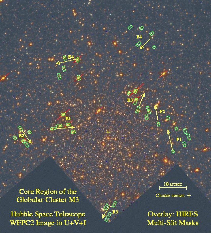
Figure 1: A portion of an HST/WFPC2 image of the core of M3. This color composite is based on archival F336W ($U$), F555W ($V$), and F814W ($I$) exposures. Eight HIRES multi-slit masks are overlaid, B1–B4 targeting bright stars and F1–F4 targeting mostly faint stars. For each mask, the arrow originates from the slitlet designated #1 (e.g., B1.1, B2.1, etc.) and points in the direction of increasing slitlet number for the rest of the slitlets in that mask. North is up and east is left. Saturation bleeds are visible in the $I$- and $V$-band images for the brightest red giants. The seeing FWHM was about $0.8\arcsec$ during the HIRES observations, whereas the resolution of the WFPC2 image is $0.1\arcsec$. Thus, crowding and contamination are more problematic in the spectroscopic data than is apparent from this image. The bright blue spots and streaks correspond to cosmic ray hits. The exposure time was longest in F336W so this image has the largest number of such hits. The PC1 CCD appears to have the highest surface density of hits but that is simply because it has a higher pixel density on this color image than the WF CCDs.

Bright red giant targets in M3 were selected from an archival HST/WFPC2 dataset for which a stellar photometry list in the form of $V$, $V-I$ was kindly provided to us by Ben Dorman. Appropriate groups of 4–5 targets were isolated by eye and attempts were made to place each group on a multi-slit mask by optimizing the position angle and ($\Delta\alpha$, $\Delta\delta$) translation of the mask design. Four such mask designs labeled B1–B4 are shown in Figures 1 and 2. The F1–F4 mask designs shown in Figure 1 contain fainter M3 targets, mostly horizontal branch stars, which will be discussed in a later paper. Only one star observed with the F1–F4 masks, F2.4, was a red giant bright enough to be included in the present study. For each mask, the targets/slitlets were numbered in order increasing in the direction of the arrow shown in Figure 1; this numbering scheme led to the star names B1.1–B4.5, F2.4 (Table 1) adopted for this paper. Alignment stars were selected around each mask; no spectra are obtained for alignment stars and they are permitted to lie outside the $\approx 10\arcsec\times 15\arcsec$ slitmask area occupied by spectroscopic targets. Of the 42 M3 stars actually observed in the Keck I program, 23 were RGB members recorded with sufficient S/N to warrant abundance analysis: six single-slit stars, 16 stars on the B1–B4 masks, and one star on the F1–F4 masks.

The fabrication of HIRES multi-slit echelle masks was carried out by Bill Mason at Keck Observatory under the supervision of Jeff Lewis of the Lick Observatory instrument shops. Masks were milled onto an aluminum plate with a highly polished surface, designed to serve as a flat mirror for the TV guider camera system. Each slitlet was milled as a rectangle whose corners were rounded because of the finite diameter ($0.5\arcsec$) of the milling tool. At the location of each alignment star, a non-reflective “blind” spot was etched into the otherwise reflective surface by drilling the mill tool halfway into the thickness of the aluminum plate (small bold symbols overlaid on stellar symbols in Figure 2. The aluminum mask plate can accommodate nine multi-slit masks arranged side by side, any one of which can be placed in the HIRES light path by rotating the wheel containing the mask plate.

After a mask was selected, and the telescope pointed at the desired coordinates at the correct sky position angle, mask alignment was achieved by ensuring that the blind spots were centered on the corresponding alignment stars on the TV guider image. Only translational offsets were needed for this procedure; fine tuning of the position angle was never needed. The exposure times for masks B1, B3, and B4 given in Table 1 are the sum of three individual integrations, that of B2 the sum of two integrations, and F2 that of a single integration. A uniform sequence of short TV guider camera frames was saved; coadding these frames allows us to obtain estimates of the seeing and telescope pointing/mask alignment during the main spectroscopic exposure. For the purposes of wavelength calibration, arc lamp exposures were obtained through each mask. Moreover, radial velocity standard stars were observed through one or more slitlets of each mask.

2.3 Reduction of the Multi-slit Spectra

The extraction of stellar spectra in multi-slit echelle data generally used the same procedure as single-slit data. The key differences were in the defining and tracing of the extraction apertures of individual stars within a given mask and the lack of sky subtraction.

As the red giants in our study are relatively bright, identifying the target stars in a cross-dispersion plot of the CCD image is straightforward. The cross-dispersion plot revealed slight overlap between the adjacent slitlets in each order. To minimize the effect of contamination between neighboring stars/slitlets, the widths of the extraction apertures were hand-defined. The quartz flat-field frames were reduced using the same apertures, as regions with cross-contamination would show up in having $\approx 2\times$ more counts than normal in the cross-dispersion plots. These quartz frames, and later the extracted Th/Ar spectra, were inspected to ensure that there was no cross-contamination between apertures. Unlike the case of the single-slit, no sky background apertures were defined as there were no appropriate blank regions.

For the masks with the longest overall slit lengths ($\sim 9^{\prime\prime}$), there was slight overlap between the bluest adjacent echelle orders for the end slitlets. In such cases, the overlapping data in those regions were simply discarded. Otherwise there were 29 full orders per exposed spectrum, each with four or five slitlets, resulting in 116 or 145 extraction apertures per exposure.

Scattered light was removed by fitting to the inter-order regions of the exposed spectrum. Generally the maximum of the subtracted surface was on the order of 30 counts per pixel, which is a few percent of the counts per pixel in the stellar continuum.

The final one-dimensional spectra were extracted using a variance-weighting scheme. The extraction of the Th/Ar arc lamp spectra was accomplished using the same aperture definitions as the target stars. As a check of the aperture definitions, the extracted arc lamp spectra were inspected for signs of contamination from adjacent apertures; they generally passed this test with the exception of “bleeds” from very strong, overexposed features.

3 ABUNDANCE ANALYSIS

3.1 Keck I HIRES Spectra of M3 Giants

Analysis of these spectra proceeded along the lines of earlier papers in the series by the Lick-Texas group (LTG) (see, e.g., Kraft et al. 1997, Sneden et al. 1997), but modified in accordance with practices introduced in the LTG paper on M5 (Ivans et al. 2001) and discussed extensively in the recent review article by Kraft & Ivans (2003). Briefly, the observed colors provided a first estimate of T_eff, making use of the $(B-V)^{\rm 0}$ or $(V-K)^{\rm 0}$ (when available) versus T_eff scales of Alonso et al. (1999, Table 6), which are in turn based on the IR-Flux method (Blackwell et al. 1990). Values of log $g$ were estimated by assigning to each giant a mass of 0.80$M_{\odot}$, assuming an M3 true distance modulus $(m-M)^{\rm 0}$ = 15.02 (Kraft & Ivans 2003), applying Worthey’s (1994) bolometric corrections, and calculating the surface gravity from the fundamental relationship $g$ $\sim$ $\mathcal{M}$T_eff⁴/L.

As before, we employed MARCS models (Gustafsson et al. 1975) and the current version of the MOOG line analysis code (Sneden 1973) to compute abundances from the EWs on a line by line basis. The resulting plot of log $\epsilon$(Fe) versus the excitation potential of each Fe I line (hereafter called the “Fe I excitation plot”) was then used iteratively to “correct” the preliminary estimates of T_eff, and the models run again until the Fe I excitation plot showed a zero slope, i.e., the value of log $\epsilon$(Fe) showed no dependence on Fe I excitation potential. Values of the microturbulent velocity, v_t, were estimated in the usual way by inspection of a plot of log $\epsilon$(Fe) versus EWs of the Fe I lines.

We proceeded as just outlined out of concerns expressed in the recent literature that estimates of metallicity based on Fe I might not be reliable because of the possible overionization of Fe inherent in the atmospheres of metal-poor stars (Thevenin & Idiart 1999, Asplund & Garcia Perez 2001). Fe is mostly singly-ionized in the atmospheres of globular cluster giants, so “Fe overionization” has little effect on the abundance of Fe II. In addition, Fe II abundances have been shown to remain virtually unaffected if 3D calculations replace 1D calculations (Asplund & Garcia Perez 2001); this may not be the case for Fe I (Nissen et al. 2002). For these reasons, we have based our “metallicity estimates” on log $\epsilon$(Fe), derived from the Fe II lines in the spectra. We make no attempt to derive values of log $g$ by forcing equality between log $\epsilon$(Fe) from Fe I and log $\epsilon$(Fe) from Fe II. Rather we fix log $g$ from the estimated value of T_eff, mass, and cluster distance modulus, i.e., from evolutionary considerations, with the consequence that log $\epsilon$(Fe) from Fe I and Fe II may differ.

Despite the concerns about Fe I, Kraft & Ivans (2003) found that the value of T_eff derived from the Fe I excitation plot agreed closely with the value of T_eff obtained from the T_eff versus color scales of Alonso et al. (1999). This is an empirical result, obtained from the analysis of giants in seven globular clusters having small reddening [$E(B-V)$ $\leq$ 0.10]. An offset toward higher T_eff’s by $\sim$50-100 K would be required in the case of the Houdashelt et al. (2000) scale. Adoption of this alternate scale would reduce the abundance of Fe based on Fe II by $\simeq$0.04 dex. Since in this paper we are concerned largely with the comparison of abundances of Fe in M3 and M13, we adopt the Alonso et al. scale, the difference in abundance being independent of the choice of T_eff.

In Table 3 we list the adopted model parameters, Fe I and Fe II abundances and radial velocities for the 23 M3 giants observed in the Keck I HIRES program. Also listed are photometric parameters and radial velocities for three stars that were excluded from the abundance analysis: B2.2, a warmer AGB star with poor S/N in its spectrum; B2.5 a much hotter star, for which no photometric parameter estimation was attempted; and B3.1, whose spectrum was compromised by that of a second star displaced slightly blueward. The columns labeled T_eff(spec) and log $g$(spec) are values found by adjusting the photometric estimates in accordance with the Fe I excitation plot. The radial velocities were obtained with reference to the night sky O₂ doublets, as discussed in the paper on NGC 7006 (Kraft et al. 1998, Appendix A). These will not be discussed further here, as we will later include measurement of velocities derived from the remaining 18 Keck I spectra in a separate paper. Values of [Fe/H] derived from Fe I and Fe II do not include the small adjustments (+0.05 dex and +0.02 dex, respectively) in log $gf$ that Kraft & Ivans (2003) found necessary to reproduce the solar Fe abundance [log $\epsilon$(Fe) = 7.52], using Kurucz models without convective overshoot (Castelli et al. 1997, Peterson et al. 2003) plus the Oxford log $gf$ values (Blackwell et al. 1980). Again our concern is the comparison of M3 with M13; we adopt the same set of log $gf$ values for all stars in both clusters. The mean values of [Fe/H] derived from Fe I and Fe II, respectively, are –1.58 ($\sigma$ = 0.06) and –1.45 ($\sigma$ = 0.03), which implies an Fe I “underabundance factor” of –0.13 dex. We assume that the “metallicity” of M3 is given by the abundance of Fe based on Fe II.

In Table 4 we list the values of [X/Fe] for elements from O to Eu again from the Keck I data; mean values for this sample are given at the bottom of the table. The star-to-star abundance scatters of elements with atomic weights $A$ $\geq$ $A$(Si) provide reasonable internal uncertainty estimates of these abundance values. For more detailed discussion of overall uncertainties the reader is referred to Sneden et al. (1997) and Ivans et al. (1999,2001).

The abundance of O is derived from spectrum synthesis of the [O I] doublet at 6300, 6364 Å. Allende Prieto, Lambert, & Asplund (2001) have re-considered the solar O abundance from the 6300.3 Å line, pointing out that a high-excitation (E.P. = 4.27 eV) Ni I line is a substantial contaminant. But in our cool giant stars, the Ni I contribution to the [O I] is very small, and can be ignored. Test calculations suggest that typically EW(Ni I) $\leq$ 0.5 mÅ, while EW([O I]) ranges from $\sim$20 to $\sim$70 mÅ.

Since O is entirely in the neutral state but Fe is mostly ionized, we normalized the [O/Fe] ratio to [Fe/H] derived from Fe II (Kraft & Ivans 2003). For consistency with the earlier studies of M13 and halo field giants, we retained the Anders & Grevesse (1989) “traditional” solar oxygen abundance of log $\epsilon$(O) = 8.93 instead of the revised value of 8.69 recommended by Allende Prieto et al. (2001). All other elements, from Na through Eu, are mostly in the singly ionized state in the atmospheres of globular cluster giants, but only Sc, Ti, Ba, La and Eu abundances are actually derived from lines in that state. We therefore normalized those elements to the abundance of Fe based on Fe II.

The other elements make their appearance in the spectrum in lines of the neutral state, and presumably also suffer from “overionization” if indeed Fe is so affected. It therefore seems best to normalize those to [Fe/H] based on Fe I All [Na/Fe] ratios are derived from spectrum synthesis of the Na I doublet at 5682, 5688 Å and EW measurements of the doublet at 6154, 6160 Å.

Finally, we also list in Table 4 [Na/Fe] ratios taking into account the non-local thermodynamic equilibrium (nLTE) versus log $g$ corrections recommended by Gratton et al. (2000), from a study of metal-poor halo field stars.

3.2 Lick Hamilton Spectra of M3 Giants

Somewhat lower resolution (R $\sim$ 30000) Lick 3.0m Hamilton spectra of 10 M3 giants had already been analyzed by members of LTG and reported in the literature (Kraft et al. 1992, 1993, 1995). We reanalyzed seven of these spectra, assigning slightly revised values of T_eff and log $g$ based on the precepts outlined above in §3.1. The earlier work did not include estimates of [X/Fe] for Sc (based on Sc I), Mn, Ba and Eu; these are added here. We also derive estimates of [Na/Fe] taking into account nLTE effects. We compute V, Mn, and Ba abundances with full accounting for hyperfine substructure, following the recipe outlined in Ivans et al. (2001) for V I and Ba II lines, and adopting the hyperfine data of Kurucz (1995) for the Mn I 6021.79 Åline. Table 5 contains the adopted models and values of [Fe/H] derived from Fe I and Fe II. Table 6 has derived [X/Fe] ratios for all elements except Mg, Al, Ti (based on Ti II) and La, the lines of which fell in the interstices between the echelle orders and thus were not recorded. Three stars (MB1, vZ 297, III-28) of the Lick sample were dropped, the S/N of the spectra having been judged inadequate.

Two stars, AA and vZ 1397, were analyzed from both Lick and Keck I spectra. These stars were used to compare the EWs derived from the two investigations. It was found that the Keck I HIRES spectra produced lines that, on the average, were 7% smaller in EW compared with Lick Hamilton spectra; before re-analyzing the Lick data, we reduced the EWs of all lines by that amount. We also used these two stars to study any possible offsets in abundance. In Tables 5 and 6 we interline for these two stars the Keck I data taken from Tables 3 and 4. For AA, the agreement in [Fe/H] for both Fe I and Fe II is excellent, as are the common [X/Fe] ratios, the largest difference being 0.09 dex for [Sc/Fe] derived from Sc I (based on one line). For vZ 1397, the agreement is less good, and it is driven principally by the 0.11 dex difference in [Fe/H] derived from Fe II. Since the S/N and spectral resolution of the Keck I spectra exceed that of the Lick Hamilton spectra, we give precedence to the abundances derived from the former.

The mean abundance ratios for the seven Lick stars are given at the bottom of of Table 6. The mean values of [Fe/H] derived from Fe I and Fe II are –1.55 ($\sigma$ = 0.02) and –1.46 ($\sigma$ = 0.05) respectively, in excellent agreement with the mean values determined from the Keck I data (Table 3). Inclusion of the Lick Hamilton stars brings the total number of M3 giants available for discussion to 28.

3.3 Revised Abundances for M13 Giants

Again using the precepts described in §3.1, we re-assigned values of T_eff and log $g$ to 18 of the 21 M13 giants that were observed either with the post-1995 version of the Lick Hamilton spectrograph (R $\sim$ 50000) or the HIRES spectrograph of the Keck I telescope (R $\sim$ 45000) (Kraft et al. 1997); the three stars omitted had spectra of relatively low S/N. As before, we adopted the Alonso et al. (1999) T_eff scale based on $(B-V)^{\rm 0}$ (Cudworth & Monet 1979) and/or $(V-K)^{\rm 0}$ (Cohen et al. 1978) when available, and took a distance modulus for M13 of $(m-M)^{\rm 0}$ = 14.42 (discussed by Kraft & Ivans 2003). Adjustments to [Fe/H] determined from both Fe I and Fe II lines and to [X/Fe] values were determined from the offsets in Table 3 of Ivans et al. (2001); the offsets themselves remain nearly constant with small changes in metallicity (in this case $\sim$0.3 dex) (see also Shetrone 1996). We also determined abundances of Ba, La and Eu, elements that had not been included in the earlier analysis. Results are listed in the top portion of Table 7, but are restricted to elements of particular interest in the comparison of M13 and M3 (in this case, O, Na, Mg, Al, Ba, La and Eu). In the lower portion of Table 7, we exhibit corresponding results for the remaining 16 giants that had been studied earlier, based entirely on Hamilton spectra of lesser resolution (R $\sim$ 30000). For these, only O and Na abundances (in addition to [Fe/H]) are given.

Only one star, L835, is common to both the Keck I and Lick samples. In this case, the agreement in the value of [Fe/H] based on Fe I is disappointingly poor, but the situation is much better for Fe II. The values of [X/Fe] for O and Na, however, are in excellent agreement. As with M3, we prefer the values based on the superior S/N and spectral resolution of the Keck I observations.

Mean values of the abundances are found at the bottom of Table 7. For the Keck I sample alone, the values of $\rm\langle[Fe/H]\rangle$ based on Fe I and Fe II lines are –1.62 ($\sigma$ = 0.06) and –1.55 ($\sigma$ = 0.09), respectively. Corresponding values using the Lick sample only are –1.57 ($\sigma$ = 0.07) and –1.50 ($\sigma$ = 0.09). The small differences most likely spring from the lower resolution and generally poorer S/N of the Lick, compared with Keck I spectra. In any case, the Fe I “overionization” deficiency appears to be $\sim$0.08 dex, based on this analysis procedure.

4 DISCUSSION

The major concern of this paper centers on the remarkable contrast of certain [X/Fe] ratios among giants in M3 in comparison with comparably-evolved giants in M13, on the one hand, and the halo field giants on the other. We divide the discussion into the familiar groups by nucleosynthetic origin, and discuss M3 stars along with their M13 and halo field surrogates within each group. We do not, in any one of these cases, have a “complete” sample of stars selected by $M_{\rm V}^{\rm 0}$. Brighter than $M_{\rm V}^{\rm 0}$ = –1.5, we have high resolution analyses for 19 giants in M3 and 22 giants in M13. Total sample sizes in M3 and M13 are 28 and 32, respectively; in each cluster, our sample includes a few stars having $M_{\rm V}^{\rm 0}$ $>$ –0.5. We therefore regard our two samples, comparable in size, as at least representative, and therefore anticipate that larger samples will not lead to unexpected surprises.

4.1 Fe-peak and Heavier Elements

Existing research on cluster abundances indicates that there is little star-to-star intracluster variation in [X/Fe] ratios for elements having atomic weights $A$ $\geq$ $A$(Si). There are, of course, exceptions, most notably among $r$-process species in the very metal-poor cluster M15 (Sneden et al. 1997, Sneden et al. 1999). There are also cases in which $\rm\langle[X/Fe]\rangle$ differs significantly from one cluster to another at a similar value of [Fe/H], as for example, the substantial differences in Si, Ba, La and Eu that exist when one compares M4 with M5 (Ivans et al. 2001). These variations emerge when stellar sample sizes are moderately large (N $\gtrsim$ 20), and since our M3 and M13 samples exceed this number, we begin by exhibiting in Figure 3 the [X/Fe] ratios for Si and heavier elements versus T_eff for the M3 stars of Table 4 and 6, and M13 stars of Table 7. Horizontal dashed lines refer to the mean values of [X/Fe] for M3 stars only.

Inspection of Figure 3 and examination of the accidental errors tabulated at the feet of Tables 4, 6, and 7 suggests that the spread in [X/Fe] is for the most part small and attributable to a paucity of lines (in the cases of, e.g., Sc II, Ba II, La II, Eu II) and/or line weakness (EW $<$ 10 mÅ, e.g., for V I, La II, Eu II). Exceptions appear to be the very high abundances of La and Ba abundances in two different M13 giants, and the very low value of Eu in a single M3 giant (B4.4). None of these stars exhibit unusual abundances of other elements. The data of Figure 3 also show that the mean values of [X/Fe] in M3 and M13 differ no more than $\sim$0.1 dex. In addition, the pattern also follows that of field halo stars with metallicities [Fe/H] $\sim$ –1.5 (Fulbright 2002), with the possible exception of Ba, which on average appears to be about 0.15 dex more Ba-rich in both clusters compared with the field. On the other hand, [Eu/Fe] in both clusters is quite close to the mean value for field stars.

4.2 Interrelated C, N, and O Abundances

Carbon and nitrogen abundances were obtained for a substantial sample of CN-weak and CN-strong giants in both M3 and M13 in a pioneering study by Suntzeff (1981). A number of these stars were reanalyzed by Smith et al. (1996) who, coupling these results with what were then freshly determined values of [O/Fe] (Kraft et al. 1992,1993), examined whether the relative abundance of these species was consistent with CNO tricycle processing. Their cyanogen-band index S(3839) was shown to be anticorrelated with [C/Fe] and [O/Fe], and correlated with [N/Fe]; they concluded that the strength of the cyanogen band was driven largely by the abundance of N. Further modeling led them to conclude that [C/Fe] and [O/Fe] were correlated, whereas [N/Fe] remained anticorrelated with both [C/Fe] and [O/Fe] (their Figure 5). They also found that the total abundance C+N+O was, within the errors, essentially the same for all stars in both M3 and M13. These results support the view that the behavior of C, N, and O is compatible with CNO tricycle processing.

The new M3 oxygen abundances reported here add only a small amount of additional information, largely because the newly analyzed stars, lying as they do mostly near the center of M3, are not the ones studied previously for C and N abundances. Included among stars with newly derived [O/Fe]_II ratios are I-21, IV-77, IV-101, and A. Although they have known S(3839) indices, only I-21, IV-77, and IV-101 have freshly derived carbon abundances (Pilachowski et al. (2003). In addition, oxygen abundances for M3 giants previously analyzed by Kraft et al. (1992,1993) have been somewhat revised in this paper. In Figure 4 we plot both the revised and newly derived abundances of [O/Fe]_II against S(3839). The anticorrelation is morphologically the same as that found previously by Smith et al. (1996). The reader should note that M3 and M13 stars lie along the same locus, but in contrast with M13, there are no M3 stars with very low oxygen abundance.

In Figure 5, we plot also the oxygen versus carbon correlation, following Smith et al. (1996), but with the revised oxygen abundances tabulated here, plus the new carbon abundances for the three M3 stars noted above. The results are in the expected direction: whenever oxygen is depleted via CNO processing, carbon also is depleted, and the abundances are correlated. There is a slight hint that at a given [O/Fe]_II, [C/Fe] is slightly smaller in M13 than in M3.

The conclusion that the relationship between C, N, and O abundances is consistent with CNO tricycle processing does not, reveal the site of the corresponding nucleosynthetic reshuffling. However, Suntzeff’s (1981) early study showed that $\rm\langle[C/Fe]\rangle$ declined with evolutionary state along the first giant branches of both M3 and M13. In the case of M3, this result was strengthened owing to a recent study by Smith et al. (2002a). These authors found that $\rm\langle[C/Fe]\rangle$ declines from $\sim$–0.2 at $M_{V}$ $\sim$ +0.6 to $\sim$–1.1 at $M_{V}$ $\sim$ –2.3 (the red giant tip). They also detected a slight offset in carbon abundances between CN-weak and CN-strong stars: $\rm\langle[C/Fe]\rangle$ was –0.14 lower in the CN-weak group. Plotting Suntzeff’s M13 data on top of the M3 data (Figure 6), we find a similar decline in $\rm\langle[C/Fe]\rangle$ (albeit with larger scatter) over the same luminosity range. Additionally, the M13 giants achieve even lower carbon abundances than do their M3 counterparts (by $\sim$0.2 dex). Even more striking is the result of Briley et al. (2003). They found a range of [C/Fe] values from –0.8 to 0.0 among main sequence turnoff stars in M13, but at the same time found that $\rm\langle[C/Fe]\rangle$ declined from $\sim$–0.4 at the main sequence to the value of $\sim$–1.3 obtained earlier by Suntzeff for stars at the red giant tip.

Owing to stellar flux limitations, nothing is known of oxygen and nitrogen abundances among main sequence members of either M3 or M13. However, the spread in [C/Fe] among these stars in M13 suggests that CNO processing must have occurred in material that was incorporated in these stars before they achieved their present evolutionary state. Nevertheless, there is no escaping the fact that, on the average, $\rm\langle[C/Fe]\rangle$ declines as M13 and M3 stars evolve above $M_{V}$ $\sim$ +0.6, the luminosity level at which the hydrogen shell burns through the molecular weight discontinuity left behind from the deepest penetration of the outer convection zone (the so-called red giant “bump”).

Among halo field giants, $\rm\langle[C/Fe]\rangle$ also begins to decline at the same red giant “bump” luminosity (Gratton et al. 2000), but contrary to the situation in M3 and M13, the degree of carbon depletion at its most severe does not exceed –0.7, and averages about –0.5. This limit is strikingly similar to the highest [C/Fe] ratios seen among giants in M3 and M13 (see Figure 5). It is therefore perhaps not surprising to find that, among halo field giants, Gratton et al. (2000) found no change in [O/Fe] with advancing evolutionary state, fixed at a value of $\rm\langle[O/Fe]\rangle$ = +0.34.

In Figure 7 we illustrate [O/Fe]_II as a function of $M_{\rm V}^{\rm 0}$ in M3 (Tables 4 and 6) and M13 (Table 7). Our samples contain no stars with $M_{\rm V}^{\rm 0}$ $\gtrsim$ +0.1, so we cannot test the behavior of [O/Fe]_II at luminosities below that of the red giant bump. We can describe the distribution of the stars brighter than $M_{\rm V}^{\rm 0}$ = +0.1, by dividing them into two groups near log $g$ = 0.8 ($M_{\rm V}^{\rm 0}$ $\sim$ –1.7), and by introducing three levels of oxygen “deficiency”. Typically among halo field giants near [Fe/H] = –1.5, [O/Fe]_II lies in the range 0.0 to +0.5 (average near +0.3), and we speak of these as “oxygen-normal”. Those in the clusters with 0.0 $>$ [O/Fe]_II $>$ –0.4, we call “oxygen-poor”. Finally we refer to those in the range –0.4 $>$ [O/Fe]_II $>$ –1.2 as “super oxygen-poor”.

Of the 11 M3 stars having $M_{\rm V}^{\rm 0}$ $>$ –1.7, nine (82%) are O-normal and two (18%) are O-poor; there are no super-O-poor stars in this range. The absence of super-O-poor stars is also a characteristic of the 16 brighter M3 stars. The split among normal and O-poor stars in this group is 72% to 28%, respectively, roughly similar to the lower luminosity group. (We arbitrarily assigned one star, B.4.2, having [O/Fe]_II = 0.00 to the “normal” group.) The situation in M13 is not so different for the 11 stars in the fainter group: 73% are O-normal, 18% are O-poor, and one star (I-12) is super-O-poor. But among the stars of the brighter group, the situation is dramatically different. Of the 23 brighter stars, only seven (30%) are O-normal, nine (39%) are O-poor, and seven (30%) are super-O-poor. (Again we arbitrarily assign one star, L261, having [O/Fe]_II = 0.00 to the “normal” group). Six of the nine super-O-poor stars are brighter than $M_{\rm V}^{\rm 0}$ = –2.3, and are therefore essentially at the tip of the giant branch.

We summarize the results of this section as follows:

1. Metal-poor halo stars, whether in the field or in such clusters as M3 and M13, all show a decline in $\rm\langle[C/Fe]\rangle$ starting when stars evolve through the red giant bump. This is superimposed on top of a pre-existing spread in [C/Fe] exhibited among main sequence and turnoff stars at least in M13, and one would not be surprised if this were true also in M3 (although this is not yet observationally demonstrated). A spread in [C/Fe] is found also among field halo subdwarfs (Gratton et al. 2000), but it appears to be smaller than that found among main sequence and turnoff stars in M13.

2. The decline is driven by stellar evolution and presumably results from the deep mixing of envelope material through the region just ahead of the H-burning shell where conversion of C to N takes place. The deficiency of $\rm\langle[C/Fe]\rangle$ among halo giants is typically –0.5 dex, but is larger in clusters, reaching –0.7 to –0.9 dex in M3 and M13.

3. We divide (somewhat arbitrarily) our sample of giants into three groups depending on the degree of oxygen deficiency: O-normal stars have [O/Fe]_II $>$ 0.0, O-poor stars lie in the range 0.0 $>$ [O/Fe]_II $>$ –0.4, and super-O-poor stars have [O/Fe]_II $<$–0.4. Among halo field stars, there are no O-poor or super-O-poor objects, and giants appear to have on the average the same oxygen abundances as main sequence subdwarfs (see also Gratton et al. 2000). In M3 there are no super-O-poor stars, and of the 28 giants in the sample, about one-third are O-poor. If this is attributable to O to N conversion in the material making up the envelope of some giants in M3 (either pre-existing processing or processing within the stars themselves), we conclude that both the degree and the frequency of the effect is rather mild. The situation in M13 is dramatically different: fewer than half the giants are O-normal, and of the remaining, 30% are super-O-poor. Most of these lie near the red giant tip. Indeed of the giants brighter than $M_{\rm V}^{\rm 0}$ = –2.3, 60% are super O-poor. It is hard to escape the conclusion that the majority of the brightest M13 giants mix envelope material deep enough into the H-burning shell that significant processing of O to N occurs within the stars themselves.

4.3 Interrelationships Among the Light Elements: O, Na, Mg, Al

4.3.1 The Na versus O Anticorrelation

Giants in most low metallicity globular clusters exhibit an anticorrelation of [Na/Fe] and [O/Fe], and M3 is no exception. In Figure 8, we compare our samples of giants in M3 (Tables 4 and 6) with those of M13 (Table 7), as well as giants of the halo field (Shetrone 1996, Gratton et al. 2000), the last-named group consisting of stars with [Fe/H] $<$ –1.0. Small vertical and horizontal lines drawn through the points denote stars known to be CN-strong or CN-weak, respectively (Smith 2002a,b); most field halo giants are CN-weak (Hesser et al. 1977; Langer et al. 1992). In contrast with earlier plots of this kind (e.g., Kraft 1994, his Figure 8), we have included the nLTE Na corrections recommended by Gratton et al. (2002), which have the effect of enhancing values of [Na/Fe] with increasing luminosity. We also normalize [O/Fe] to [Fe/H] based on Fe II and [Na/Fe] to [Fe/H] based on Fe I, in accordance with precepts argued by Kraft & Ivans (2003). Inspection of the three panels leads us to the following conclusions.

1. Halo field giants show no sign of a Na versus O anticorrelation. There is a considerable range of values of [Na/Fe]_I (–0.5 to +0.3), and a smaller range in [O/Fe]_II (0.0 to +0.6), a result noted earlier by Kraft et al. (1993), Hanson et al. (1998), and Gratton et al. (2000). Mean values of [O/Fe]_II = +0.3 and [Na/Fe]_I = –0.1 are generally regarded as numbers characteristic of Type II supernovae ejecta.

2. M13 giants exhibit a range of [Na/Fe]_I (a factor of $\sim$8) and a range of [O/Fe]_II (a factor of $\sim$25) that is larger than that seen in any other cluster (although the range in $\omega$ Cen may be comparable, see Norris & DaCosta 1995), and the anticorrelation is decidedly marked. Na and O abundances in the most Na-poor and O-rich giants of M13 are comparable to what is seen in halo field giants. As expected, these stars are CN-weak; CN-strong stars are those with deficiencies of O. In the present sample, there is a tendency for giants that are less advanced in evolutionary state (log $g$ $>$ 0.8) to favor higher [O/Fe]_II and lower [Na/Fe]_I than are found in stars nearer the red giant tip (log $g$ $<$ 0.8).

3. M3 giants exhibit an anticorrelation that is “intermediate” between the halo field and M13 stars. M3 stars follow quite closely the anticorrelation defined by the M13 stars, but “cutoff” near [O/Fe]_II = –0.2, [Na/Fe]_I = +0.5. There are no super-O-poor stars in M3, as already noted. It is also the case that the distribution of stars in the diagram is essentially independent of evolutionary state, in contrast to the situation in M13. The shape and boundaries of the M3 Na versus O distribution are, in fact, quite similar to those found recently in NGC 6752 (Yong et al. 2003), a point to which we will return in Section §4.1.1.

4.3.2 [Mg/Fe]_I versus [O/Fe]_II

Previous work (Figure 9 of Kraft et al. 1997) indicated that M13 giants with lower than average [O/Fe] also had lower than average [Mg/Fe]. In the present Figure 9, we plot [Mg/Fe]_I versus [O/Fe]_II for the sample of M13 giants of that study observed with either the Keck I HIRES spectrograph or the post-1995 version of the Lick Hamilton spectrograph. As before, we find $\rm\langle[Mg/Fe]_{I}\rangle$ = +0.22 ($\sigma$ = $\pm$ 0.09) for giants with [O/Fe]_II $>$ –0.2 whereas $\rm\langle[Mg/Fe]_{I}\rangle$ = –0.01 ($\sigma$ = 0.07) for giants with [O/Fe]_II $>$ –0.2. In Figure 9, we superimpose the O and Mg abundances for 22 of the 23 giants in our M3 sample (Table 4). One star has [O/Fe]_II $>$ –0.2, and it does not have a low Mg abundance; on the other hand, the one M3 giant (B4.5) having a very low, indeed negative, value of [Mg/Fe]_I does not have a derivable oxygen abundance (the S/N of the spectrum is too low). However, it is clearly the case that our M3 sample contains few, if any, stars with the low Mg abundances characteristic of many of the brightest giants in M13. We address later implications of the change in the abundance ratio of Mg isotopes with [O/Fe]_II among giants in M13 (Shetrone 1996b).

4.3.3 [Al/Fe]_I versus [Mg/Fe]_I

The expectation that Al may arise owing to proton captures on the various isotopes of Mg (e.g., Kraft et al. 1997, Shetrone 1996b, Ivans et al. 1999) prompts an investigation of [Al/Fe]_I versus [Mg/Fe]_I which is shown in Figure 10. All data are taken from Tables 4 and 7. We divide the stars at log $g$ = +0.8 into two groups by evolutionary state, as we did previously in the discussion of the Na versus O anticorrelation (§4.2). Although the sample sizes are small, the distribution suggests that in each cluster there are two groups with distinctly differing Al abundances. Whereas the higher and lower luminosity giants are distributed among the two groups about equally in the case of M3, the distribution appears to be quite different in the case of M13, with most of the brighter giants lying in the group with high Al abundances. The highest Al abundances in M13 also appear to be about a factor of two higher than the highest Al abundances in M3.

Generally speaking, the observational accuracy of our Al abundances, which are based on two lines of moderate EW and excitation potential, is likely higher than that of our Mg abundances, which are based on one or two rather strong lines of rather high excitation potential. This may in part account for the rather displeasing result that the M3 giants of higher luminosity seems to have [Mg/Fe]_I ratios that are on average about 0.1 dex higher than the stars of lower luminosity (omitting the anomalous star (B4.5) with a negative [Mg/Fe]_I ratio). The result suggests the presence of a systematic error in our adopted T_eff or log $g$ scales, as a function of luminosity. If an arbitrary adjustment to correct the effect in M3 were also applied to the sample of stars in M13, it would strengthen the conclusion that the more luminous M13 giants have a lower Mg abundance than the less luminous stars. However, the same conclusion would be reached even if such a correction were not applied to the M13 sample.

4.3.4 [Al/Fe]_I versus [Na/Fe]_I

As expected, these two “odd-elements” are correlated in both M3 and M13, but in each case, there appear to be two well-separated groups (Figure 11). M3 and M13 giants satisfy essentially the same correlation, but the M13 giants extend toward higher values of both Na and Al by a factor of about two. The population of M13 stars having the highest values of Na and Al abundances is dominated by stars in the most advanced evolutionary state (log $g$ $<$ 0.8). All halo field giants considered here lie among the group of stars with lowest Na and Al abundances.

4.3.5 “Odd” versus “Even”: [Na/Fe]_I versus [Mg/Fe]_I

Hanson et al. (1998), using the the observational results of Pilachowski et al. (1996), noted that there exists a Na versus Mg correlation among halo field giants having [Fe/H] $<$ –1.0. In Figure 12 (left-hand panel), we plot [Na/Fe]_I versus [Mg/Fe]_I in these giants, the data having been “corrected” for the nLTE effect in Na. In the right hand panel of Figure 12, we plot the results of Fulbright (2002) for halo field subdwarfs, the straight line taken from a fit (by eye) of the correlation for the halo giants. The Mg abundances of Fulbright have been modified, first to eliminate all Mg lines except $\lambda$5528 and/or $\lambda$5711 (the lines used exclusively for studies of the giants), and second to allow for differences in the adopted log $gf$ values assumed by Fulbright for the 5528/5711 pair. The two panels should therefore be on the same system of Mg and Na abundances.

Inspection of the two panels of Figure 12 suggests that, (1) there is no change in the correlation whether the samples are drawn from the main sequence or from the giants, and (2) there is no change in the distribution whether one deals with giants having gravities greater or less than log $g$ = 0.8. In other words, there is no dependence of the correlation on evolutionary state among metal-poor halo field stars.

Sodium and magnesium are near neighbors in the periodic table and are believed to arise during carbon and neon burning in Type II SNe, giving rise to the so-called “odd-even” effect. The correlation suggests that there is a range in the [Na/Mg] ratio at a given metallicity, since all stars regardless of metallicity below [Fe/H] = –1.0 seem to satisfy the same correlation. Thus along the correlation, the [Na/Mg] ratio varies from –0.6 to -0.1, with a mean near –0.4; this is in quite good agreement with Arnett’s (1971) hydrostatic and explosive carbon-burning models, in which [Na/Mg] ranges from –0.8 to –0.2 for stars having [Fe/H] $<$ –1.0. The more recent models reported by Timmes et al. (1995) suggest a lower mean [Na/Mg] ratio, near –0.7, for such low-metallicity stars. We note that the stars with [Na/Mg] ratios closest to the theoretical value of Timmes et al. are the one shown by Fulbright (2002) to favor Galactic orbits having relatively high values of orbital energy and (absolute) angular momentum.

Corresponding plots of [Na/Fe]_I versus [Mg/Fe]_I for M3 and M13 are shown respectively in the left and right hand panels of Figure 13, the data being taken from Tables 4, 6, and 7. The straight line is the same as that in the two panels of Figure 12. Again we see the somewhat unpleasing result that in M3 the stars of low luminosity have systematically lower Mg abundances than the stars of higher luminosity (log $g$ $<$ 0.8), but otherwise the two kinds of giants are essentially intermixed. The giants of M13 present a rather different picture. Here the more luminous giants prefer a location well off the halo-defined line, in the direction of low Mg, high Na, whereas the lower luminosity giants, except for three exceptions (out of a sample of 10 stars) prefer a location near the normal halo line.

The effect is illustrated more dramatically in Figure 14, in which [Na/Fe]_I is plotted against [Mg/Fe]_I for M13, this time using the very much larger sample of M13 giants studied by Pilachowski et al. (1996b). The Mg abundances were adjusted slightly to conform to the system of Mg abundances adopted here (by plotting [Mg/Fe]_I values of Table 7 against the [Mg/Fe] values of Pilachowski et al. for common M13 giants), and the Na abundances adjusted for nLTE as explained earlier. Again we see that M13 giants of high luminosity are confined to the upper left-hand part of the diagram, although they do not have that domain to the exclusion of stars having log $g$ $>$ 0.8.

4.4 Implications of the Interrelationships among O, Na, Mg, and Al

4.4.1 Deep Mixing versus Primordial (or Pollution) Scenarios

In all of the interrelationships illustrated in §4.3, M13 giants inhabit a more “extreme” domain than do M3 giants, when the stars are compared at essentially the same evolutionary state. As discussed in §4.3.1, most M13 giants near the red giant tip have, in comparison with corresponding M3 giants, very low O and very high Na abundances, suggesting that first ascent M13 giants immediately prior to the He core flash undergo a period of deep mixing not experienced by similar giants in M3. But a recent study of giants in NGC 6752 (Yong et al. 2003), a cluster having [Fe/H] essentially the same as that of M3 and M13, casts doubt on such an interpretation. Thus, in what follows, we describe similarities and differences among giants in NGC 6752, M13 and M3.

From a sample of 20 (mostly) first ascent NGC 6752 giants with –1.0 $\leq$ $M_{\rm V}$ $\leq$ –2.5, Yong et al. (2003) discovered that the abundances of the minor isotopes ²⁵Mg and ²⁶Mg, relative to the dominant ²⁴Mg, were ofter higher than in the solar system (²⁴Mg:²⁵Mg:²⁶Mg = 79:10:11, Lodders 2003 and references therein) and normal stars. The minor Mg isotopes were also very much more abundant than the values predicted for the ejecta of Type II SNe (Timmes et al. (1995). For NGC 6752, Yong et al. found a range of abundance ratios running from 63:08:30 to 84:08:08, with one NGC 6752 giant (star 702) having an unusually low ratio of 53:09:39. Hydrogen-burning shell temperatures in first ascent NGC 6752 giants are too low to allow efficient operation of the reaction ²⁴Mg(p,$\gamma$)²⁵Al (Powell et al. 1999), and thus the chain of proton captures leading to the destruction of ²⁴Mg and the production of ²⁵Mg, ²⁶Mg and ²⁷Al. Therefore Yong et al. concluded that deep mixing was ruled out as a source of the anomalous Mg abundance ratios as well as the enhancement of ²⁷Al. They proposed instead a scenario in which the abundance ratios in NGC 6752 giants actually reflect those found in the ejecta of 3-6 $M_{\odot}$ cluster giants that had already evolved: either the low mass giants we presently see formed from such secularly ejected material, or their envelopes were seriously polluted or even ablated and replaced by this material. A scenario like this is supported both observationally and theoretically. On the one hand, most of the abundance anomalies in Na, Mg and Al found among NGC 6752 giants, that had earlier been attributed to deep mixing, were found to exist already in their main sequence progenitors (Gratton et al. 2001), which points to a pre-existing origin. In addition, models which predict the abundance ratios in the ejected envelope material of intermediate-mass low-metallicity AGB stars (Siess et al. 2002, Karakas & Lattanzio 2003) show that ²⁵Mg and ²⁶Mg are overproduced relative to ²⁴Mg. For example, Karakas & Lattanzio found that in the envelope of a 4 $M_{\odot}$ AGB star having Z = 0.004, there can develop a situation in which the abundances of ²⁴Mg, ²⁵Mg and ²⁶Mg are approximately equal; in a 6 $M_{\odot}$, Z = 0.004 AGB star, ²⁴Mg virtually disappears relative to the other isotopes. At the same time, hot bottom CNO cycling in the same stars can lead to an overabundance of N at the expense of O and excess production of ²³Na. Qualitatively these are just the sorts of anomalies found in the spectra of present-day NGC 6752, M3 and M13 giants.

So far, we have discussed recent results found in giants of NGC 6752. What bearing does this have on M3 and/or M13? Our M3 spectra do not have sufficient S/N near the MgH bands at $\lambda$5135 to permit discussion of the Mg isotopes. But a previous study of the MgH bands in six M13 giants (Shetrone 1996b) permits us to compare ratios of (²⁵Mg + ²⁶Mg)/²⁴Mg in M13 with NGC 6752. Shetrone’s spectra, of somewhat lower resolution than those of Yong et al.(2003), did not permit the separation of lines of ²⁵MgH from ²⁶MgH, so we resort to discussing the quantity (²⁵Mg+²⁶Mg)/²⁴Mg). In Figure 15 we plot [O/Fe]_II versus the quantity (²⁵Mg+²⁶Mg)/²⁴Mg for 19 of the 20 giants studied by Yong et al., plus the six M13 giants of Shetrone. The missing NGC 6752 star is No. 702, the one with the lowest abundance of ²⁴Mg. Yong et al. were unable to measure [O/Fe]_II for this star, owing to lower than average S/N for this spectrum.

Inspection of Figure 15 shows that there is an anticorrelation between oxygen abundance and the overabundance of the rare isotopes of Mg relative to ²⁴Mg. Further, the plot indicates that whatever is the nucleosynthetic process that depletes oxygen and enhances the rarer isotopes of Mg, NGC 6752 and M13 share in that process. Moreover, if a primordial ablation or pollution scenario is responsible for what is seen in NGC 6752, the same scenario must have operated to any even greater extent in M13. Finally, the existence of this anticorrelation means that the extreme oxygen depletion seen in M13 giants near the red giant tip is probably not a result of deep mixing.

Parallel support for this conclusion is found Figure 16, which is a replot of Figure 9, this time excluding the giants of M3, but noting the Mg abundance ratios of the six stars studied by Shetrone (1996a,b). (Because Shetrone could not resolve ²⁵Mg from ²⁶Mg, he simply assigned them equal weight in the blended spectra.) The stars of lowest oxygen abundance also have the lowest abundance of ²⁴Mg as well as the highest abundances of the rarer isotopes, as already noted by Shetrone. If the current nuclear reaction rates are correct, deep mixing again cannot be responsible for the depletion of ²⁴Mg found among most of the M13 giants of lowest oxygen abundance and highest luminosity.

What about M3? Even though we cannot report on the Mg isotopic ratios in this cluster, we can compare some key abundance-ratio plots in M3 with those of NGC 6752. The comparison is somewhat clouded by the possibility of systematic differences between investigators. For example, Yong et al. (2003) employ a completely different set of Fe I and Fe II lines compared with the set adopted in our analyses of M3 and M13. NGC 6752 stars have not been investigated by our group; as Yong et al. note, previous investigations yielded [Fe/H] ranging from –1.42 to –1.62. It seems best then, in comparing abundance ratio diagrams of NGC 6752 with those of M3 and M13, to concentrate on the morphology and recognize the possibility of zero-point differences of 0.1 or 0.2 dex in values of [X/Fe].

In the two panels of Figure 17 we compare the [Na/Fe]_I,nLTE versus [O/Fe]_II diagrams of M3 and NGC 6752. The two diagrams are morphologically quite similar, and both are remarkably different from the corresponding M13 diagram. In Figure 18, we compare the [Na/Fe]_I,nLTE versus [Mg/Fe]_I diagrams of M3 and NGC 6752, again noting that both are morphologically dissimilar to the corresponding diagram for M13 (Figure 14). M3 and NGC 6752 do not match perfectly, as one can easily see: M3 giants seem to have a larger scatter of Mg abundances. The main point is that neither cluster has the large population of giants lying far from the field giant relationship in the low Mg versus high Na regime, such as one finds in M13.

4.4.2 HB Morphology

The main difference in the morphology of the color-magnitude diagrams for these three clusters is the distribution of stars along the HB, a phenomenon usually referred to as “the second parameter problem”. The Lee et al. (1994) second parameter index is nearly the same for M13 vs NGC 6752 (0.97 versus 1.00), which indicates that the HB is very blue, whereas the value of the index for M3 is 0.08, which corresponds to a uniformly populated HB. Although age is rather widely believed to be the factor responsible for the second parameter (e.g., Sarajedini et al. 1997, Rey et al. 2001), other possibilities have been invoked. For example, if deep mixing were to significantly penetrate into the hydrogen shell burning region, evolution to the red giant tip would be slowed and the He/H ratio in the envelopes of evolving red giants would be increased (Sweigart 1997). The HB descendants would then be bluer than their unmixed counterparts. Another possibility would involve an “ab initio”, or “primordial” difference in He abundance between clusters (Johnson & Bolte 1998), perhaps brought about if the low mass giants we presently see formed from the He-enriched ejecta of 3-6 $M_{\odot}$ cluster giants (Ventura et al. 2002). Qualitatively at least, an increase in the He/H ratio would favor the development of a blue HB, all other factors being equal.

But if deep mixing were responsible for the blue HB’s of M13 and NGC 6752, and if seriously depleted O were the most significant “symptom” of the deep mixing phenomenon, then one might expect NGC 6752 to exhibit a Na vs O relationship as “advanced” as that of M13. This is clearly not the case. As we have seen, in both the Na versus O and Na versus Mg plots, NGC 6752 is much more like M3, a cluster with an “intermediate” HB morphology. However, these remarks apply only to the case in which an increase in the He/H ratio is a result of deep mixing. It does not rule out a picture in which NGC 6752 and M13 share the property of a “primordial” overabundance of He, relative to M3. It would clearly be of interest to explore the Mg isotopic ratios in M3 as a test (Ventura et al. 2002) of the He/H ratio among M3 giants close to the red giant tip.

5 SUMMARY

Previous high resolution studies, based on a small sample of stars, suggested that M3 giants had a smaller degree of chemical “peculiarity” than was the case among M13 giants, this despite the fact that the two clusters have about the same metallicity ([Fe/H] $\approx$ –1.5). The present study, based largely on high resolution Keck I spectra of 23 M3 giants, confirms the earlier conclusion vis-a-vis M13 giants. Compared with M13, M3 giants exhibit only modest deficiencies of O and enhancements of Na, less extreme enhancements of Al, fewer stars with low Mg and correspondingly high Na, and no evidence that O depletions and Na enhancements are dependent on an advancing evolutionary state as appears to be the case in M13. Field halo giants show correlated behavior of Mg and Na, consistent with an origin in supernova Type II sites either in hydrostatic or explosive carbon burning. Both M3 and M13 giants, however, also show evidence of proton capture synthesis of ²³Na from ²²Ne and ²⁷Al from proton-capture chains starting with ²⁴Mg. M3 stars appear to represent a case of proton-capture synthesis intermediate between the field and M13.

We find that giants in NGC 6752 and M13 satisfy the same anticorrelation of [O/Fe]_II with the ratio (²⁵Mg+²⁶Mg)/²⁴Mg, which is a measure of the relative contribution of rare to the abundant isotope of Mg. As Yong et al. (2003) argue, such a ratio could only have come about in nuclearly processed material ejected from cluster stars in the 3-6 $M_{\odot}$ range (Siess et al. 2002, Karakas & Lattanzio 2003). This points to a scenario in which the peculiar abundance ratios of stars in M13 and NGC 6752 arose in such ejected material and was then either incorporated into (or ablated) the atmospheres of the low-mass stars we now see in these clusters, or else these low-mass stars were formed from such ejecta. The process seems to have advanced to a much greater degree in M13 than in NGC 6752. This in turn suggests that the very low O abundances seen in M13 giants near the red giant tip are not, after all, the result of deep mixing driven by stellar evolution, but have their origin in hot-bottom CNO burning in the same 3-6 solar mass giants responsible for the overabundances of the rare isotopes of Mg. If deep mixing is not responsible for the severe O-depletion among M13 giants, then it cannot be called upon to increase the He/H ratio in the atmospheres of such stars. This suggests that the excessive blueness of the M13 HB branch is not a result of an excess He abundance due to deep mixing. It does not, of course, rule out excess He from a primordial or pollution source (Johnson & Bolte 1998, Ventura et al. 2002).

The Mg isotopic ratios among M3 giants are not known. However, the abundance anticorrelation of O and Na, and the Na vs Mg diagrams of NGC 6752 and M3 tend to be rather similar and both are unlike the same diagrams in M13.

The most interesting conclusion of this work then presents a curious conundrum. The anticorrelation of O and the Mg isotopic abundance ratio suggests that M13 giants in a very small interval of initial mass preferentially underwent severe pollution or ablation, or alternatively, were preferentially formed from material secularly ejected earlier from more massive cluster giants. These stars only just at this moment arrived essentially at the red giant tip, exactly where the effect of deep mixing, if it indeed exists, would likely be most easily manifest. It is a most remarkable coincidence, if indeed that’s what it is.

Figure 2: Schematic representation of the HIRES bright star masks B1–B4 superimposed on the M3 star field. Each target/slitlet is assigned a unique number as indicated. The schematic star field image is derived from a photometry list provided by B. Dorman and collaborators, and should bear a good resemblance to the color image shown in Figure 1 except in rare instances where the photometry list is incomplete. The symbol size is roughly proportional to apparent stellar brightness. The symbols indicate different stellar types: circle = RGB; pentagon = AGB; square = red HB; $+$ = RR Lyrae; up-triangle$\rightarrow$down-triangle$\rightarrow$3-pointed starred symbol = increasingly bluer HB stars; $\times$/asterisk = extreme/moderate blue straggler; dot = subgiant/main sequence. The small bold dots superimposed on the stellar symbols mark the locations of non-reflective marks etched on the shiny front face of each multi-slit mask plate. Mask alignment was carried out by registering these marks with the corresponding reference bright stars on the HIRES guider camera image.

Figure 3: Abundance ratios for silicon and heavier elements in M3 (filled circles) and M13 (open circles) as functions of T_eff. The ordinate of each panel has the same extent (1.2 dex), and the midpoint (indicated with a dotted line) is the mean abundance ratio of the particular element in M3.

Figure 4: Correlation of the CN band strength index S(3839) and oxygen abundances of M3 and M13 stars. In this and all succeeding figures, M3 stars will be plotted as circles and M13 stars as triangles; the symbols will be filled ones for lower gravity stars (log $g$ $\leq$ 0.8, corresponding approximately to $M_{\rm V}^{\rm 0}$ $\leq$ –1.7), and open ones for higher gravity stars. Whenever possible, in this and succeeding figures dotted horizontal and or vertical lines will be drawn to denote the solar abundance ratios of various elements.

Figure 5: Correlation of the carbon and oxygen abundances of M3 and M13 stars. Symbols and lines are as in Figure 4.

Figure 6: Correlation of the carbon abundances of M3 and M13 stars with their absolute magnitudes. Symbols and lines are as in Figure 4.

Figure 7: Correlation of the oxygen abundances of M3 and M13 stars with their absolute magnitudes. Symbols and the dotted line are as in Figure 4. The dashed horizontal line represents the dividing line between those stars designated as “oxygen-poor” and those we call “super oxygen-poor”.

Figure 8: Correlation of the sodium and oxygen abundances in field giants (top panel, “$\times$” symbols), M3 giants (middle panel), and M13 giants (bottom panel). The dotted lines are as in Figure 4, and so are the symbols for M3 and M13 stars. Vertical and horizontal lines through the M3 and M13 points denote CN-strong and CN-weak stars, respectively.

Figure 9: Correlation of the oxygen and magnesium abundances of M3 and M13 stars. Symbols and lines are as in Figure 4.

Figure 10: Correlation of the magnesium and aluminum abundances of M3 and M13 stars. Symbols and lines are as in Figure 4.

Figure 11: Correlation of the sodium and aluminum abundances of M3 and M13 stars. Symbols and lines are as in Figure 4.

Figure 12: Correlation of the sodium and magnesium abundances of field giants (left-hand panel), and field subdwarfs (right-hand panel). Different symbols are used to represent low gravity (log $g$ $\leq$ 0.8) and high gravity, while one symbol represents all subdwarfs. The dotted lines are as in Figure 4. The slanting solid lines represent the mean trend of the field giant data.

Figure 13: Correlation of the sodium and magnesium abundances of M3 and M13 stars. Symbols and dotted lines are as in Figure 4. The slanting solid lines are repeated from Figure 12.

Figure 14: Correlation of the sodium and magnesium abundances based on the Pilachowski et al. (1996) sample of M13 giants. The diagram is morphologically the same as the right-hand panel of Figure 13. The slanting solid line is that of Figure 12.

Figure 15: Correlation of [O/Fe]_II with (²⁵Mg+²⁶Mg)/²⁴Mg among giants of M13 and NGC 6752. The horizontal dotted line corresponds to the solar ratio of the sum of the rare Mg isotopes to ²⁴Mg (e.g.., Lodders 2003 and references therein).

Figure 16: A plot of [Mg/Fe]_I vs [O/Fe]_II for M13 giants. The numbers are the values of (²⁵Mg+²⁶Mg)/²⁴Mg, according to Shetrone (1996b). The giants with low oxygen abundances have Mg isotopic abundances higher than those exhibited by giants with higher oxygen abundances.

Figure 17: [Na/Fe]_I,nLTE versus [O/Fe]_II for giants in M3 and NGC 6752. The diagrams are morphologically quite similar.

Figure 18: [Na/Fe]_I,nLTE versus [Mg/Fe]_I for giants in M3 and NGC 6752. The M3 giants show a considerably wider range of Mg abundances for a given Na abundance. Although differences in abundance zero-points may exist, neither distribution is morphologically similar to the distribution in M13 (Figure 14).

Table 1: Photometry, Coordinates and Observations of M3 Giants

Star	vZ	$V$	$B-V$	$V-I$	$V-K$	$\Delta\alpha$	$\Delta\delta$	Exp	S/N
						$\arcsec$	$\arcsec$	min
I-21	1352	13.11	1.35	$\cdots$	3.10	$\cdots$	$\cdots$	15	65
IV-77	334	13.11	1.32	$\cdots$	$\cdots$	$\cdots$	$\cdots$	15	75
IV-101	265	13.18	1.35	$\cdots$	$\cdots$	$\cdots$	$\cdots$	15	110
A	640	13.27	1.26	$\cdots$	$\cdots$	$\cdots$	$\cdots$	15	75
AA	238	12.69	1.57	$\cdots$	3.43	$\cdots$	$\cdots$	15	85
$\cdots$	1397	12.65	1.56	$\cdots$	3.49	$\cdots$	$\cdots$	15	75
B1.1	911	13.69	1.32	1.22	$\cdots$	+20.52	+1.72	90	130
B1.2	898	13.50	1.22	1.22	$\cdots$	+17.60	+2.86	90	140
B1.3	893	12.74	1.50	1.58	$\cdots$	+16.44	+7.11	90	150
B1.4	887	13.12	1.34	1.31	$\cdots$	+14.68	+3.32	90	150
B1.5	874	13.65	1.22	1.23	$\cdots$	+12.65	+0.57	90	150
B2.1	$\cdots$	14.79	0.92	1.05	$\cdots$	+32.38	+2.11	60	85
B2.2	$\cdots$	14.72	0.77	0.94	$\cdots$	+34.51	–1.31	60	65
B2.3	$\cdots$	14.74	0.88	1.02	$\cdots$	+29.11	+0.88	60	40
B2.4	964	13.42	1.25	1.26	$\cdots$	+31.48	–2.39	60	105
B2.5	$\cdots$	15.69	0.12	0.58	$\cdots$	+30.27	–3.62	60	65
B3.1	$\cdots$	14.69	0.96	0.88	$\cdots$	–11.29	+8.48	90	110
B3.2	729	12.96	1.41	1.40	$\cdots$	–10.84	+12.51	90	125
B3.3	746	13.56	1.10	1.12	$\cdots$	–8.18	+15.13	90	100
B3.4	733	12.61	1.63	1.68	$\cdots$	–10.58	+15.75	90	130
B4.1	860	13.04	1.43	1.41	$\cdots$	+10.82	+27.83	85	145
B4.2	855	13.05	1.41	1.40	$\cdots$	+10.39	+20.89	85	130
B4.3	$\cdots$	14.12	0.93	1.06	$\cdots$	+15.67	+28.67	85	90
B4.4	$\cdots$	14.75	0.76	0.94	$\cdots$	+16.01	+24.64	85	75
B4.5	$\cdots$	15.44	0.76	0.94	$\cdots$	+17.68	+21.81	85	70
F2.4	$\cdots$	14.22	1.02	1.17	$\cdots$	–15.74	+8.09	60	50

Table 2: Equivalent Widths of M3 Giants

$\lambda$	ID	E.P.	log $gf$	(1)	(2)	(3)	(4)	(5)	(6)	(7)	(8)	(9)	(10)	(11)	(12)	(13)	(14)	(15)	(16)	(17)	(18)	(19)	(20)	(21)	(22)	(23)
6300.31	[O I]	0.00	–9.75	54	44	26	46	34	70	18	26	69	24	30	18	9	22	25	37	72	57	42	15	13	$\cdots$	9
6363.79	[O I]	0.02	–10.25	22	22	15	20	11	37	7	11	33	11	8	5	8	6	9	11	36	27	16	$\cdots$	$\cdots$	$\cdots$	2
6154.23	Na I	2.10	–1.56	11	7	20	10	28	18	12	12	17	22	6	4	13	13	24	7	15	13	15	9	$\cdots$	$\cdots$	$\cdots$
6160.75	Na I	2.10	–1.26	17	11	30	20	43	29	18	17	29	37	15	6	$\cdots$	22	39	5	27	23	27	18	4	10	16
5528.42	Mg I	4.35	–0.36	165	160	174	168	189	197	148	162	205	175	153	121	104	156	178	151	203	187	173	125	103	94	126
5711.09	Mg I	4.34	–1.63	$\cdots$	$\cdots$	$\cdots$	100	105	101	73	84	111	98	70	$\cdots$	$\cdots$	$\cdots$	$\cdots$	$\cdots$	$\cdots$	100	93	56	40	27	49
6696.03	Al I	3.14	–1.57	$\cdots$	$\cdots$	$\cdots$	$\cdots$	$\cdots$	26	$\cdots$	$\cdots$	$\cdots$	$\cdots$	8	$\cdots$	$\cdots$	33	59	$\cdots$	$\cdots$	$\cdots$	$\cdots$	$\cdots$	$\cdots$	12	17
6698.67	Al I	3.14	–1.89	5	5	35	7	45	12	17	13	15	28	5	10	$\cdots$	18	34	3	12	11	20	11	8	14	10
5793.08	Si I	4.93	–2.06	$\cdots$	$\cdots$	$\cdots$	$\cdots$	20	22	20	17	24	19	19	14	14	18	$\cdots$	19	21	25	23	13	8	$\cdots$	13
6142.49	Si I	5.62	–1.48	10	7	$\cdots$	9	10	10	9	7	13	10	10	5	9	6	7	8	8	13	10	7	5	$\cdots$	8
6145.02	Si I	5.61	–1.37	12	8	13	13	11	14	11	9	12	11	12	$\cdots$	$\cdots$	11	11	12	10	15	11	11	$\cdots$	7	7
6243.82	Si I	5.61	–1.27	22	16	21	17	12	$\cdots$	12	14	$\cdots$	14	11	$\cdots$	9	15	17	13	13	15	14	8	9	12	11
6244.48	Si I	5.61	–1.27	12	10	16	19	14	17	14	12	17	16	12	11	$\cdots$	17	17	11	6	21	18	$\cdots$	$\cdots$	13	13
5590.12	Ca I	2.51	–0.71	$\cdots$	$\cdots$	$\cdots$	91	106	117	$\cdots$	74	114	93	74	60	48	77	$\cdots$	$\cdots$	115	106	95	58	48	44	61
5867.56	Ca I	2.92	–1.57	$\cdots$	$\cdots$	$\cdots$	20	21	28	11	10	27	16	11	9	$\cdots$	11	$\cdots$	9	24	23	18	$\cdots$	$\cdots$	$\cdots$	$\cdots$
6161.30	Ca I	2.52	–1.27	68	62	67	67	81	93	50	39	95	67	47	34	22	44	76	41	85	77	71	28	17	20	39
6166.44	Ca I	2.52	–1.14	74	69	75	77	86	99	53	49	101	73	53	34	30	54	73	48	89	84	76	34	20	21	42
6169.04	Ca I	2.52	–0.80	94	89	92	91	113	125	76	69	119	93	72	54	42	73	96	67	115	105	96	48	30	39	56
6169.56	Ca I	2.52	–0.48	106	103	110	107	128	136	90	88	136	107	87	74	57	86	112	82	130	120	111	65	46	49	71
6455.60	Ca I	2.52	–1.29	58	57	61	59	77	89	45	40	85	60	43	30	21	41	63	33	79	69	65	19	12	18	37
6471.66	Ca I	2.51	–0.69	$\cdots$	$\cdots$	$\cdots$	103	119	132	81	81	131	103	78	68	55	85	$\cdots$	75	127	112	107	56	34	38	66
6499.65	Ca I	2.52	–0.82	100	89	92	99	116	126	77	69	122	95	73	55	49	74	96	65	121	103	98	53	29	37	62
6508.84	Ca I	2.51	–2.41	$\cdots$	$\cdots$	$\cdots$	$\cdots$	16	17	$\cdots$	5	14	10	6	$\cdots$	$\cdots$	8	$\cdots$	$\cdots$	17	13	11	$\cdots$	$\cdots$	$\cdots$	$\cdots$
6305.67	Sc I	0.02	–1.28	$\cdots$	$\cdots$	$\cdots$	37	90	136	15	$\cdots$	122	38	$\cdots$	$\cdots$	$\cdots$	$\cdots$	$\cdots$	8	136	65	$\cdots$	$\cdots$	$\cdots$	$\cdots$	$\cdots$
5526.82	Sc II	1.77	–0.03	$\cdots$	$\cdots$	$\cdots$	96	106	100	86	100	110	100	90	75	55	100	$\cdots$	85	105	98	101	86	64	45	73
6279.74	Sc II	1.50	–1.16	51	39	41	45	58	54	38	40	56	45	38	30	19	39	49	35	56	53	54	26	17	23	$\cdots$
6309.90	Sc II	1.50	–1.52	13	17	18	27	32	35	24	22	38	24	21	10	10	21	26	21	33	28	27	14	9	$\cdots$	$\cdots$
5866.45	Ti I	1.07	–0.84	$\cdots$	$\cdots$	$\cdots$	101	142	163	70	66	165	99	68	44	26	73	$\cdots$	63	179	122	113	31	18	21	51
5922.11	Ti I	1.05	–1.47	$\cdots$	$\cdots$	$\cdots$	70	104	125	42	33	122	68	34	20	10	37	$\cdots$	24	130	87	80	10	$\cdots$	11	30
5965.83	Ti I	1.88	–0.41	$\cdots$	$\cdots$	$\cdots$	57	91	100	36	30	102	58	31	17	15	29	$\cdots$	27	94	71	66	11	$\cdots$	$\cdots$	29
5978.54	Ti I	1.87	–0.50	$\cdots$	$\cdots$	$\cdots$	52	74	91	28	22	86	47	25	15	$\cdots$	25	$\cdots$	22	85	65	56	12	$\cdots$	8	24
6064.63	Ti I	1.05	–1.94	$\cdots$	$\cdots$	$\cdots$	42	71	90	17	14	85	39	19	11	7	17	$\cdots$	13	93	56	46	$\cdots$	$\cdots$	$\cdots$	10
6303.77	Ti I	1.44	–1.57	33	22	38	27	54	68	14	10	68	28	12	5	7	9	37	9	68	39	37	$\cdots$	$\cdots$	$\cdots$	10
6312.24	Ti I	1.46	–1.55	$\cdots$	18	43	30	36	73	12	7	64	18	10	9	$\cdots$	12	28	13	69	40	32	$\cdots$	$\cdots$	$\cdots$	12
6606.97	Ti II	2.06	–2.79	$\cdots$	$\cdots$	$\cdots$	25	25	27	16	19	24	23	15	13	$\cdots$	17	$\cdots$	13	23	21	22	16	$\cdots$	$\cdots$	12
6233.20	V I	0.28	–2.00	34	29	34	33	63	86	12	7	85	29	13	5	4	12	38	$\cdots$	90	45	39	$\cdots$	$\cdots$	6	$\cdots$
6274.66	V I	0.27	–1.69	48	40	46	46	91	113	19	15	105	48	19	$\cdots$	$\cdots$	19	58	14	111	68	59	$\cdots$	6	$\cdots$	$\cdots$
6285.16	V I	0.28	–1.56	58	42	56	55	95	114	25	15	113	51	21	7	$\cdots$	19	59	14	119	72	64	$\cdots$	$\cdots$	$\cdots$	11
6292.82	V I	0.29	–1.52	59	45	60	59	100	121	26	19	125	54	25	7	$\cdots$	22	67	15	132	74	68	6	$\cdots$	6	16
6504.19	V I	1.18	–1.23	15	8	17	15	27	41	$\cdots$	$\cdots$	34	15	5	$\cdots$	$\cdots$	$\cdots$	17	$\cdots$	37	21	18	$\cdots$	$\cdots$	$\cdots$	$\cdots$
6021.79	Mn I	3.08	+ 0.03	$\cdots$	$\cdots$	$\cdots$	81	100	111	59	54	109	77	57	32	18	57	$\cdots$	51	106	90	87	29	16	16	45
5501.48	Fe I	0.96	–3.05	187	183	190	184	233	249	155	168	258	185	151	120	100	164	195	147	259	211	199	127	92	81	121
5506.79	Fe I	0.99	–2.79	$\cdots$	$\cdots$	$\cdots$	$\cdots$	$\cdots$	$\cdots$	$\cdots$	$\cdots$	$\cdots$	$\cdots$	$\cdots$	122	106	190	$\cdots$	151	$\cdots$	$\cdots$	$\cdots$	134	94	82	128
5522.45	Fe I	4.21	–1.40	$\cdots$	$\cdots$	$\cdots$	30	32	38	21	19	39	26	17	15	$\cdots$	18	$\cdots$	21	34	35	30	$\cdots$	$\cdots$	$\cdots$	$\cdots$
5560.21	Fe I	4.43	–1.04	$\cdots$	$\cdots$	$\cdots$	31	37	40	24	25	42	31	25	20	12	24	$\cdots$	24	35	34	37	14	$\cdots$	11	20
5586.77	Fe I	3.37	–0.14	160	148	155	152	175	178	135	145	186	154	139	115	95	153	158	138	189	162	$\cdots$	120	90	88	117
6079.01	Fe I	4.65	–0.97	$\cdots$	$\cdots$	$\cdots$	25	24	30	19	16	30	26	17	$\cdots$	11	16	$\cdots$	15	26	28	25	$\cdots$	8	$\cdots$	17
6151.62	Fe I	2.18	–3.37	90	81	83	84	104	115	63	63	115	84	62	42	24	67	88	55	113	96	91	33	11	17	44
6157.73	Fe I	4.07	–1.26	63	57	61	62	71	73	44	45	80	58	46	30	23	47	63	42	$\cdots$	69	65	$\cdots$	15	19	31
6159.38	Fe I	4.61	–1.97	$\cdots$	$\cdots$	$\cdots$	5	$\cdots$	$\cdots$	$\cdots$	$\cdots$	7	5	$\cdots$	$\cdots$	$\cdots$	$\cdots$	5	$\cdots$	$\cdots$	$\cdots$	$\cdots$	$\cdots$	$\cdots$	$\cdots$	$\cdots$
6165.36	Fe I	4.14	–1.47	35	31	34	34	39	46	24	19	45	33	20	13	9	20	34	16	39	36	37	11	5	$\cdots$	19
6226.74	Fe I	3.88	–2.22	22	17	17	$\cdots$	26	28	13	11	$\cdots$	19	14	$\cdots$	$\cdots$	14	23	11	$\cdots$	$\cdots$	19	6	$\cdots$	$\cdots$	10
6229.23	Fe I	2.84	–3.00	59	54	53	53	65	74	37	35	76	53	34	18	$\cdots$	35	55	28	67	61	57	14	$\cdots$	$\cdots$	22
6240.66	Fe I	2.22	–3.23	85	77	83	80	103	113	61	65	112	83	57	34	22	61	88	49	109	94	90	27	12	14	43
6246.32	Fe I	3.60	–0.88	113	102	108	107	126	129	93	98	126	109	90	72	61	96	114	87	121	117	114	75	51	50	75
6280.62	Fe I	0.86	–4.37	139	130	138	141	182	193	106	110	190	138	106	78	52	115	147	94	195	153	154	66	33	31	77
6290.97	Fe I	4.73	–0.76	33	31	35	38	39	47	22	23	44	34	24	17	12	28	36	22	38	41	36	$\cdots$	$\cdots$	$\cdots$	23
6297.80	Fe I	2.22	–2.74	117	116	121	113	137	142	94	99	151	114	90	68	47	97	120	88	146	122	120	63	41	38	68
6301.50	Fe I	3.65	–0.72	115	105	115	113	128	127	93	102	130	107	93	70	59	96	112	98	123	117	111	82	58	50	85
6302.49	Fe I	3.69	–1.15	88	84	84	83	101	100	73	72	103	83	69	52	39	67	87	67	94	89	86	45	30	32	58
6311.51	Fe I	2.83	–3.22	45	33	42	38	57	59	$\cdots$	24	58	40	27	13	11	24	43	19	58	49	43	10	$\cdots$	$\cdots$	17
6355.04	Fe I	2.84	–2.29	99	92	104	95	119	127	76	76	129	99	74	58	48	78	103	70	121	106	104	42	21	28	60
6380.75	Fe I	4.19	–1.40	44	40	44	36	44	50	29	25	54	42	25	19	$\cdots$	30	43	25	43	46	43	12	9	$\cdots$	22
6419.96	Fe I	4.73	–0.24	60	55	61	57	64	68	46	45	69	56	43	37	32	48	62	41	60	60	59	38	19	25	36
6421.35	Fe I	2.28	–1.94	155	150	153	150	182	195	132	138	198	155	125	99	96	142	161	123	202	165	162	103	79	61	100
6494.98	Fe I	2.40	–1.24	$\cdots$	$\cdots$	$\cdots$	190	224	228	162	169	240	190	156	121	107	172	$\cdots$	157	237	208	197	133	93	80	130
6498.94	Fe I	0.96	–4.69	126	114	119	117	151	163	86	89	167	119	82	53	37	91	122	70	167	132	127	48	23	22	64
6574.23	Fe I	0.99	–5.02	103	93	95	95	130	142	64	62	143	96	59	32	18	67	100	51	140	113	101	28	13	$\cdots$	45
6593.88	Fe I	2.44	–2.42	$\cdots$	$\cdots$	$\cdots$	126	146	147	98	102	154	122	92	$\cdots$	63	103	$\cdots$	94	152	133	127	69	43	48	77
6609.12	Fe I	2.56	–2.69	$\cdots$	$\cdots$	$\cdots$	98	113	117	76	78	128	95	73	51	48	77	$\cdots$	64	121	108	102	45	29	22	60
6733.15	Fe I	4.64	–1.43	$\cdots$	$\cdots$	$\cdots$	11	17	19	8	7	17	12	6	$\cdots$	$\cdots$	8	$\cdots$	$\cdots$	14	12	11	$\cdots$	$\cdots$	$\cdots$	5
6750.15	Fe I	2.42	–2.62	$\cdots$	$\cdots$	$\cdots$	113	135	143	92	93	140	111	88	67	65	98	$\cdots$	79	141	120	123	67	29	35	69
6149.25	Fe II	3.89	–2.72	23	26	22	20	22	23	22	26	22	22	20	21	16	27	25	25	20	22	25	24	23	17	18
6369.46	Fe II	2.89	–4.25	20	20	19	18	15	19	14	18	18	15	16	$\cdots$	$\cdots$	19	17	18	17	16	15	17	13	$\cdots$	12
6416.93	Fe II	3.89	–2.79	16	25	19	19	28	25	22	22	25	24	19	17	16	24	23	22	22	23	23	19	23	16	15
6456.39	Fe II	3.90	–2.08	57	51	55	44	46	39	50	51	45	48	49	46	38	63	48	55	45	50	50	53	44	38	46
6516.08	Fe II	2.89	–3.45	54	45	49	46	48	50	48	52	51	47	45	39	39	56	47	47	42	49	49	50	39	33	40
6175.37	Ni I	4.09	–0.53	22	25	28	26	30	34	19	17	30	25	18	10	8	17	27	17	26	28	25	10	7	$\cdots$	17
6176.82	Ni I	4.09	–0.53	33	34	36	40	38	44	$\cdots$	26	42	34	27	$\cdots$	14	25	39	33	39	39	37	13	8	12	22
6177.25	Ni I	1.83	–3.50	28	24	29	31	41	44	18	17	47	25	17	6	6	13	32	22	44	36	32	$\cdots$	$\cdots$	$\cdots$	9
6378.26	Ni I	4.15	–0.89	$\cdots$	16	18	16	17	20	9	9	17	13	8	$\cdots$	13	12	14	8	19	15	16	6	$\cdots$	$\cdots$	$\cdots$
6586.33	Ni I	1.95	–2.81	$\cdots$	$\cdots$	$\cdots$	71	84	90	47	44	92	64	44	29	30	50	$\cdots$	40	87	79	71	21	9	13	34
6643.64	Ni I	1.68	–2.01	$\cdots$	$\cdots$	$\cdots$	139	162	167	109	113	174	135	105	85	65	119	$\cdots$	99	174	150	144	76	46	44	89
6767.78	Ni I	1.83	–2.17	$\cdots$	$\cdots$	$\cdots$	119	138	140	94	99	151	115	93	74	54	102	$\cdots$	86	150	125	122	67	41	42	74
5853.69	Ba II	0.60	–1.01	114	110	123	120	135	135	99	114	156	118	101	89	64	116	123	106	149	127	121	111	73	51	77
6141.73	Ba II	0.70	–0.08	165	166	169	172	201	197	146	178	227	167	152	135	106	171	177	161	218	189	180	167	127	82	120
6496.91	Ba II	0.60	–0.38	170	170	173	170	197	200	148	173	225	170	144	115	110	167	174	145	219	183	179	165	108	$\cdots$	120
6390.49	La II	0.30	–1.41	$\cdots$	$\cdots$	$\cdots$	33	35	38	19	18	49	27	16	9	$\cdots$	22	$\cdots$	15	41	37	31	14	$\cdots$	$\cdots$	13
6774.33	La II	0.13	–1.75	$\cdots$	$\cdots$	$\cdots$	28	33	38	$\cdots$	15	51	26	16	12	$\cdots$	15	$\cdots$	$\cdots$	48	40	27	$\cdots$	$\cdots$	$\cdots$	$\cdots$
6645.13	Eu II	1.37	+ 0.20	32	28	39	38	42	38	28	26	48	32	25	15	9	30	32	22	45	42	34	15	4	81	20

Table 3: Model Parameters, Fe Metallicities, and Radial Velocities of M3 Giants

Star	Teff	log $g$	Teff	log $g$	$v_{t}$	[Fe/H]	[Fe/H]	$v_{R}$
	K,phot	phot	K,spec	spec	km s-1	I	II	km s-1
I-21	4150	0.72	4175	0.70	1.70	–1.52	–1.42	–146.9
IV-77	4225	0.88	4300	0.85	1.80	–1.52	–1.43	–147.7
IV-101	4150	0.72	4200	0.75	1.70	–1.50	–1.43	–145.6
A	4200	0.80	4200	0.90	1.65	–1.52	–1.44	–151.1
AA	3975	0.45	3975	0.20	1.95	–1.57	–1.45	–150.3
vZ 1397	3950	0.40	3925	0.10	2.00	–1.53	–1.42	–147.2
B1.1	4340	1.14	4400	1.10	1.50	–1.56	–1.47	–171.9
B1.2	4340	1.06	4400	1.10	1.80	–1.62	–1.50	–152.1
B1.3	3950	0.40	3900	0.00	2.05	–1.54	–1.42	–150.9
B1.4	4190	0.79	4175	0.70	1.70	–1.58	–1.46	–146.6
B1.5	4290	1.08	4350	1.10	1.50	–1.67	–1.47	–147.0
B2.1	4750	1.83	4625	1.65	1.20	–1.61	–1.47	–146.6
B2.2	4950	1.80	$\cdots$	$\cdots$	$\cdots$	$\cdots$	$\cdots$	–157.0
B2.3	4825	1.85	4800	2.10	1.40	–1.70	–1.50	–149.8
B2.4	4275	1.05	4450	1.00	1.90	–1.59	–1.47	–146.7
B2.5	$\cdots$	$\cdots$	$\cdots$	$\cdots$	$\cdots$	$\cdots$	$\cdots$	–147.1
B3.1	4620	1.60	$\cdots$	$\cdots$	$\cdots$	$\cdots$	$\cdots$	–155.9
B3.2	4100	0.65	4175	0.70	1.75	–1.51	–1.43	–146.5
B3.3	4530	1.09	4550	1.30	1.65	–1.55	–1.45	–149.9
B3.4	3900	0.34	3850	0.00	2.00	–1.62	–1.40	–140.2
B4.1	4075	0.60	4075	0.40	1.70	–1.54	–1.46	–149.7
B4.2	4090	0.61	4100	0.40	1.70	–1.56	–1.48	–144.5
B4.3	4740	1.44	4650	1.40	1.60	–1.75	–1.50	–151.7
B4.4	4950	1.80	5050	2.00	1.50	–1.71	–1.48	–154.9
B4.5	4950	2.08	5100	2.40	1.00	–1.58	–1.47	–147.2
F2.4	4550	1.72	4600	1.70	1.20	–1.54	–1.45	–140.4

Table 4: Abundance Ratios in 23 M3 Giants Observed with Keck I HIRES

Star	O	Na	Na,rev	Mg	Al	Si	Ca	Sc	Sc	Ti	Ti	V	Mn	Ni	Ba	La	Eu
	[I]	I	I	I	I	I	I	I	II	I	II	I	I	I	II	II	II
I-21	+0.22	–0.23	–0.03	+0.19	$\cdots$	+0.27	+0.23	–0.14	–0.39	+0.22	+0.23	–0.05	–0.33	–0.08	+0.11	0.00	+0.52
IV-77	+0.22	–0.28	–0.10	+0.25	–0.18	+0.22	+0.27	–0.06	–0.28	+0.24	+0.25	+0.02	–0.31	–0.05	+0.14	+0.09	+0.51
IV-101	–0.14	+0.17	+0.37	+0.12	+0.89	+0.32	+0.21	–0.10	–0.16	+0.22	+0.25	+0.02	–0.33	–0.06	+0.25	+0.06	+0.64
A	+0.19	–0.19	–0.01	+0.31	+0.05	+0.30	+0.25	–0.09	–0.03	+0.19	+0.33	–0.03	–0.36	+0.02	+0.32	+0.25	+0.75
AA	–0.24	+0.32	+0.57	+0.37	+0.97	+0.28	+0.22	+0.09	–0.12	+0.19	+0.14	–0.06	–0.35	–0.06	+0.11	–0.03	+0.56
1397	+0.13	–0.08	+0.18	+0.32	+0.18	+0.35	+0.26	$\cdots$	–0.02	+0.31	+0.15	0.00	–0.30	–0.07	-0.02	–0.04	+0.43
B1.1	–0.08	+0.06	+0.23	+0.18	+0.68	+0.26	+0.24	–0.10	–0.06	+0.15	+0.06	–0.09	–0.37	–0.10	+0.23	+0.10	+0.63
B1.2	+0.06	–0.03	+0.14	+0.34	+0.67	+0.26	+0.22	$\cdots$	–0.06	+0.13	+0.20	–0.13	–0.37	–0.05	+0.28	+0.08	+0.57
B1.3	+0.09	–0.10	+0.16	+0.44	+0.24	+0.38	+0.19	+0.20	–0.16	+0.23	+0.04	–0.09	–0.35	–0.08	+0.26	+0.11	+0.57
B1.4	–0.17	+0.29	+0.49	+0.38	+0.82	+0.31	+0.26	–0.07	–0.10	+0.14	+0.22	–0.05	–0.38	–0.06	+0.17	+0.10	+0.57
B1.5	+0.14	–0.04	+0.13	+0.26	+0.14	+0.37	+0.25	$\cdots$	–0.05	+0.11	+0.11	–0.06	–0.36	–0.04	+0.23	+0.04	+0.57
B2.1	+0.18	–0.23	–0.15	+0.20	+0.60	+0.23	+0.26	$\cdots$	–0.10	+0.18	+0.26	–0.18	–0.42	–0.09	+0.43	+0.14	+0.51
B2.3	+0.09	–0.17	–0.11	+0.05	$\cdots$	+0.45	+0.21	$\cdots$	–0.17	+0.32	$\cdots$	+0.27	–0.60	+0.08	+0.08	$\cdots$	+0.44
B2.4	–0.06	+0.22	+0.38	+0.08	+0.79	+0.28	+0.24	$\cdots$	–0.13	+0.18	+0.09	–0.02	–0.35	–0.05	+0.18	+0.07	+0.59
B3.2	–0.18	+0.26	+0.46	+0.17	+0.89	+0.24	+0.23	+0.03	–0.08	+0.22	+0.14	0.00	–0.33	–0.05	+0.18	+0.08	+0.56
B3.3	+0.27	–0.11	+0.03	+0.20	–0.04	+0.26	+0.20	–0.12	–0.11	+0.21	+0.03	–0.08	–0.35	–0.01	+0.29	+0.04	+0.53
B3.4	+0.13	–0.15	+0.12	+0.44	+0.15	+0.27	+0.15	$\cdots$	–0.22	+0.25	+0.04	–0.08	–0.34	–0.03	+0.17	–0.02	+0.51
B4.1	+0.15	–0.09	+0.13	+0.40	+0.27	+0.38	+0.28	+0.03	–0.12	+0.22	+0.12	–0.07	–0.36	–0.05	+0.23	+0.18	+0.67
B4.2	0.00	+0.03	+0.25	+0.31	+0.58	+0.31	+0.24	$\cdots$	–0.08	+0.18	+0.13	–0.08	–0.35	–0.07	+0.21	+0.03	+0.53
B4.3	–0.10	+0.34	+0.42	+0.22	+0.83	+0.38	+0.22	$\cdots$	–0.09	+0.06	+0.22	–0.18	–0.33	–0.06	+0.63	+0.13	+0.43
B4.4	+0.22	+0.14	+0.12	+0.12	+0.84	+0.35	+0.18	$\cdots$	+0.03	+0.21	$\cdots$	$\cdots$	–0.40	–0.06	+0.27	$\cdots$	–0.04
B4.5	$\cdots$	+0.11	+0.11	–0.13	+0.81	+0.37	+0.22	$\cdots$	–0.06	+0.32	$\cdots$	$\cdots$	–0.47	0.00	+0.22	$\cdots$	$\cdots$
F2.4	+0.02	+0.09	+0.22	+0.03	+0.50	+0.19	+0.21	$\cdots$	+0.12	+0.27	+0.18	–0.10	–0.38	–0.03	+0.25	+0.19	+0.68
Cluster Mean Abundances
$<>$	+0.15	+0.01	+0.18	+0.22	+0.51	+0.30	+0.23	–0.03	–0.11	+0.21	+0.16	–0.04	–0.37	–0.05	+0.21	+0.09	+0.54
$\pm$	0.03	0.04	0.04	0.03	0.08	0.01	0.01	0.03	0.02	0.01	0.02	0.02	0.01	0.01	0.02	0.02	0.03
$\sigma$	0.15	0.19	0.20	0.15	0.36	0.06	0.03	0.11	0.10	0.06	0.09	0.08	0.06	0.04	0.11	0.09	0.15
No.	22	23	23	23	21	23	23	11	23	23	20	21	23	23	23	20	22

Table 5: Models for M3 Giants Analyzed from Old Lick Spectra

Star	Teff	log $g$	$v_{t}$	[Fe/H]	[Fe/H]
	K		km s-1	I	II
vZ 1397 (old)	3925	0.10	2.00	–1.53	–1.53
vZ 1397 (new)	3925	0.10	2.00	–1.53	–1.42
MB3	3925	0.20	1.90	–1.57	–1.48
MB4	3950	0.40	2.00	–1.55	–1.42
AA (old)	3975	0.20	2.00	–1.53	–1.43
AA (new)	3975	0.20	1.95	–1.57	–1.45
II-46	4050	0.40	1.95	–1.57	–1.52
vZ 1000	4125	0.60	1.90	–1.58	–1.41
vZ 1127	4200	0.85	1.65	–1.51	–1.43

Table 6: Revised Abundances from Old Lick Spectra of M3 Giants

Star	O	Na	Na	Si	Ca	Sc	Sc	Ti	V	Mn	Ni	Ba	Eu
	[I]	I	I,rev	I	I	I	II	I	I	I	I	II	II
1397 (old)	+0.31	0.00	+0.25	+0.45	+0.22	+0.26	–0.14	+0.27	+0.03	–0.35	–0.07	+0.01	+0.61
1397 (new)	+0.13	–0.08	+0.18	+0.35	+0.26	$\cdots$	–0.02	+0.31	0.00	–0.30	–0.07	–0.02	+0.43
MB3	+0.21	–0.21	+0.05	+0.54	+0.17	+0.26	–0.08	+0.21	–0.01	–0.28	–0.02	–0.11	+0.66
MB4	+0.12	+0.27	+0.52	+0.42	+0.24	+0.29	–0.21	+0.17	–0.17	–0.33	–0.12	+0.22	+0.72
AA (old)	–0.20	+0.30	+0.04	+0.21	+0.20	0.00	–0.15	+0.14	–0.08	–0.44	–0.14	+0.19	+0.64
AA (new)	–0.24	+0.32	+0.57	+0.28	+0.22	+0.09	–0.12	+0.19	–0.06	–0.35	–0.06	+0.11	+0.56
II-46	+0.32	–0.20	+0.03	+0.21	+0.15	+0.14	–0.20	+0.21	–0.01	–0.40	–0.14	–0.06	+0.31
1000	–0.12	+0.10	+0.31	+0.23	+0.23	–0.05	–0.24	+0.12	+0.04	–0.30	–0.03	+0.06	+0.68
1127	+0.25	–0.08	+0.12	+0.11	+0.16	–0.19	–0.20	+0.07	–0.10	–0.49	–0.04	+0.16	+0.58
Cluster Mean Abundances, Old Data Only
$<>$	+0.13	+0.03	+0.19	+0.31	+0.20	+0.10	–0.17	+0.17	–0.04	–0.37	–0.08	+0.07	+0.60
$\pm$	0.09	0.08	0.07	0.06	0.01	0.07	0.02	0.03	0.03	0.03	0.02	0.05	0.05
$\sigma$	0.21	0.21	0.18	0.16	0.04	0.19	0.05	0.07	0.08	0.08	0.05	0.13	0.14

Table 7: Abundances for M13 Giants

Star	Teff	log $g$	[Fe/H]	[Fe/H]	[O/Fe]	[Na/Fe]	[Na/Fe],rev	[Mg/Fe]	[Al/Fe]	[Ba/Fe]	[La/Fe]	[Eu/Fe]
			I	II	[I]	I	I	I	I	II	II	II
Abundances from HIRES on Keck I and Upgraded Hamilton spectrograph on Lick 3m
L598	3900	0.30	–1.62	–1.47	+0.13	–0.03	+0.23	+0.28	+0.26	+0.11	–0.05	+0.31
L629	4010	0.36	–1.63	–1.60	–0.13	+0.27	+0.51	+0.22	+0.70	+0.18	+0.05	+0.49
I-48	3950	0.34	–1.57	–1.56	–0.78	+0.45	+0.70	–0.08	+1.17	–0.07	+0.13	+0.52
II-67	3900	0.37	–1.63	–1.35	–1.00	+0.42	+0.68	+0.02	+1.16	+0.12	–0.11	+0.39
IV-25	3975	0.38	–1.64	–1.36	–1.08	+0.56	+0.80	+0.08	+1.21	+0.12	–0.13	+0.34
II-90	3960	0.38	–1.63	–1.59	–0.47	+0.37	+0.62	+0.06	+1.10	+0.35	+0.01	+0.45
L835	4035	0.45	–1.60	–1.47	–0.70	+0.46	+0.69	+0.01	+1.14	+0.21	+0.04	+0.42
J3	4520	1.31	–1.63	–1.62	–0.10	+0.53	+0.68	+0.15	+0.91	+0.30	+0.22	+0.52
A1	4550	1.34	–1.72	–1.67	+0 30	+0.01	+0.15	+0.34	+0.18	+0.28	+0.38	+0.69
I-12	4610	1.46	–1.58	–1.60	–0.47	+0.29	+0.42	–0.04	+1.18	+0.28	+0.14	+0.52
IV-19	4610	1.52	–1.62	–1.56	+0.20	–0.10	+0.03	+0.25	+0.10	+0.26	+0.08	+0.43
IV-22	4750	2.12	–1.50	–1.46	–0.25	+0.34	+0.42	–0.13	+1.04	+0.32	+0.18	+0.55
II-9	4680	1.75	–1.60	–1.61	+0.11	–0.21	–0.12	+0.16	+0.11	+0.18	+0.15	+0.42
II-41	4650	1.62	–1.54	–1.59	+0.25	–0.17	–0.06	+0.14	+0.02	+0.08	+0.15	+0.43
I-72	4825	1.97	–1.67	–1.57	+0.26	–0.21	–0.15	+0.08	$<$–0.02	+0.25	+0.34	+0.87
II-28	4750	1.57	–1.77	–1.66	+0.29	–0.02	+0.05	+0.25	$<$+0.10	+0.24	+0.21	+0.64
II-1	4850	2.05	–1.58	–1.62	$\cdots$	+0.33	+0.38	–0.20	+0.94	+0.38	–0.06	+0.46
I-54	5050	1.74	–1.64	–1.62	+0.15	+0.33	+0.36	+0.37	+0.71	+0.64	+0.28	+0.38
Abundances from Older Hamilton spectrograph on Lick 3m
L324	3925	0.35	–1.60	–1.25	–0.04	+0.33	+0.58	$\cdots$	$\cdots$	$\cdots$	$\cdots$	$\cdots$
III-56	4000	0.42	–1.64	–1.52	–0.15	+0.28	+0.52	$\cdots$	$\cdots$	$\cdots$	$\cdots$	$\cdots$
L835	4035	0.45	–1.40	–1.42	–0.73	+0.42	+0.65	$\cdots$	$\cdots$	$\cdots$	$\cdots$	$\cdots$
L853	4030	0.48	–1.65	–1.57	–0.01	+0.35	+0.58	$\cdots$	$\cdots$	$\cdots$	$\cdots$	$\cdots$
L940	4050	0.48	–1.51	–1.40	–0.57	+0.32	+0.55	$\cdots$	$\cdots$	$\cdots$	$\cdots$	$\cdots$
III-63	4120	0.60	–1.66	–1.42	–0.10	+0.39	+0.61	$\cdots$	$\cdots$	$\cdots$	$\cdots$	$\cdots$
L261	4150	0.60	–1.55	–1.63	0.00	+0.22	+0.43	$\cdots$	$\cdots$	$\cdots$	$\cdots$	$\cdots$
L262	4125	0.60	–1.56	–1.53	+0.07	+0.17	+0.38	$\cdots$	$\cdots$	$\cdots$	$\cdots$	$\cdots$
II-34	4140	0.63	–1.64	–1.64	–0.22	+0.54	+0.75	$\cdots$	$\cdots$	$\cdots$	$\cdots$	$\cdots$
III-73	4210	0.69	–1.57	–1.56	+0.25	–0.05	+0.15	$\cdots$	$\cdots$	$\cdots$	$\cdots$	$\cdots$
I-13	4230	0.80	–1.55	–1.49	+0.24	–0.16	+0.03	$\cdots$	$\cdots$	$\cdots$	$\cdots$	$\cdots$
II-76	4250	0.80	–1.65	–1.50	+0.30	–0.27	–0.09	$\cdots$	$\cdots$	$\cdots$	$\cdots$	$\cdots$
III-59	4290	0.85	–1.51	–1.55	–0.47	+0.29	+0.47	$\cdots$	$\cdots$	$\cdots$	$\cdots$	$\cdots$
III-52	4275	0.87	–1.63	–1.48	–0.23	+0.32	+0.50	$\cdots$	$\cdots$	$\cdots$	$\cdots$	$\cdots$
II-33	4300	0.90	–1.53	–1.55	+0.30	+0.05	+0.23	$\cdots$	$\cdots$	$\cdots$	$\cdots$	$\cdots$
III-18	4330	0.95	–1.52	–1.58	–0.26	+0.44	+0.62	$\cdots$	$\cdots$	$\cdots$	$\cdots$	$\cdots$
II-57	4350	1.00	–1.53	–1.48	–0.09	+0.33	+0.50	$\cdots$	$\cdots$	$\cdots$	$\cdots$	$\cdots$
Cluster Mean Abundances
$<>$			–1.60	–1.53	–0.13	+0.21	+0.39	+0.11	+0.75	+0.24	+0.11	+0.49
$\pm$			0.01	0.02	0.06	0.04	0.05	0.03	0.11	0.03	0.03	0.03
$\sigma$			0.06	0.09	0.38	0.24	0.27	0.11	0.44	0.15	0.14	0.13
No.			34	34	33	34	34	18	16	18	18	18

References

- (1) Allende Prieto, C., Lambert, D. L., & Asplund, M. 2001, ApJ, 556, L63
- (2) Alonso, A., Arribas, S., & Mart nez-Roger, C. 1999, A&AS, 140, 261
- (3) Anders, E., & Grevesse, N. 1989, Geochim. Cosmochim Acta, 53, 197
- (4) Asplund, M., & Garc a Pérez, A. E. 2001, A&A, 372, 601
- (5) Bellman, S., Briley, M. M., Smith, G. H., & Claver, C. F. 2001, PASP, 113, 326
- (6) Blackwell, D. E., Shallis, M. J., & Simmons, G. J. 1980, A&A, 81, 340
- (7) Blackwell, D. E., Petford, A. D., Arribas, S., Haddock, D. J., & Selby, M. J. 1990, MNRAS, 232, 396
- (8) Briley, M. M., Bell, R. A., Hesser, J. E. & Smith, G. H. 1994, Can. J. Phys., 72, 772
- (9) Briley, M. M., Bell, R. A., Hoban, S., & Dickens, R. J. 1990 ApJ, 359, 307
- (10) Briley, M. M., Smith, V. V., Suntzeff, N. B., Lambert, D. L., Bell, R. A., & Hesser, J. E. 1996, Nature, 383, 604
- (11) Briley, M. M., Cohen, J. G., & Stetson, P. B. 2003, ApJ, 579, L17
- (12) Buonanno, R., Corsi, C. E., Buzzoni, A., Cacciari, C., Ferraro, F. R., & Fusi Pecci, F. 1994, A&A, 290, 69
- (13) Cannon, R. D., Croke, B. F. W., Bell, R. A., Hesser, J. E., & Stathakis, R. A. 1998, MNRAS, 298, 601
- (14) Castelli, F., Gratton, R. G., & Kurucz, R. L. 1997, A&A, 318, 841
- Cavallo & Nagar (2000) Cavallo, R. M .& Nagar, N. M. 2000, AJ, 120, 1364
- (16) Cavallo, R. M., Sweigart, A. V., & Bell, R. A. 1996, ApJ, 464, L79
- (17) Cavallo, R. M., Sweigart, A. V., & Bell, R. A. 1998, ApJ, 492, 575
- (18) Cohen, J. G. 1999, AJ, 117, 2434
- (19) Cohen, J. G., Briley, M. M., & Stetson, P. B. 2002, AJ, 123, 2525
- (20) Cohen, J. G., Persson, S. E. & Frogel, J. A. 1978, ApJ, 222, 165
- (21) Cottrell, P. L., & Da Costa, G. S. 1981, ApJ, 245, 79
- (22) Cudworth, K. M. 1979, AJ, 84, 1312
- (23) Cudworth, K. M., & Monet, D. G. 1979, AJ, 84, 774
- (24) Da Costa, G. S. 1998, in The Stellar Content of Local Group Galaxies, IAU Symp. 192, ed. P. Whitelock, R. Cannon San Francisco: Ast. Soc. Pac.), p. 13
- (25) Denissenkov, P. A., Da Costa, G. S., Norris, J. E., & Weiss, A. 1998, A&A, 333, 926
- (26) Denissenkov, P. A. & Denissenkova, S. N. 1990, Sov. Astr. Lett., 16, 275
- (27) Dorman, B. 1998, private communication
- (28) Fitzpatrick, M. J. & Sneden, C. 1987, BAAS, 19, 1129
- (29) Fulbright, J. P. 2000, AJ, 120, 1841
- (30) Fulbright, J. P. 2002, AJ, 123, 404
- (31) Gratton, R. G., Sneden, C., Carretta, E. & Bragaglia, A. 2000, A&A, 354, 169
- (32) Gratton, R. G., et al. 2001, A&A, 369, 87
- (33) Gustafsson, B., Bell, R. A., Eriksson, K., & Nordlund, A. 1975, A&A, 42, 407
- (34) Hanson, R. B., Sneden, C., Kraft, R. P., & Fulbright, J. 1998, AJ, 116, 1286
- (35) Hesser, J. E., Hartwick, F. D. A., & McClure, R. D. 1977, ApJS, 33, 471
- (36) Houdashelt, M. L., Bell, R. A., & Sweigart, A. V. 2000, AJ, 119, 1448
- (37) Iben, I. & Renzini, A. 1984, Phys. Rev., 105, 329
- (38) Ivans, I. I.,Kraft, R. P., Sneden, C., Smith, G. H., Rich, R. M., & Shetrone, M. D. 2001, AJ, 122, 1438
- (39) Ivans, I. I., Sneden, C., Kraft, R. P., Suntzeff, N. B., Smith, V. V., Langer, G. E. & Fulbright, J. P. 1999, AJ, 118, 1273
- (40) Johnson, J. A., & Bolte, M. 1998, AJ, 115, 693
- (41) Karakas, A. I., & Lattanzio, J. C. 2004, ApJ, submitted
- (42) King, J. R., Stephens, A., Boesgaard, A. M., Deliyannis, C. 1998, AJ, 115, 666
- (43) Kraft, R. P. 1994, PASP, 106, 553
- (44) Kraft, R. P., & Ivans, I. I. 2003, PASP, 115, 143
- (45) Kraft, R. P., Sneden, C., Langer, G. E., & Prosser, C. F. 1992, AJ, 105, 645
- (46) Kraft, R. P., Sneden, C., Langer, G. E., & Shetrone, M. D. 1993, AJ, 106, 1490
- (47) Kraft, R. P., Sneden, C., Langer, G. E., Shetrone, M. D.m & Bolte, M. 1995, AJ, 109, 2586
- (48) Kraft, R. P., Sneden, C., Smith, G. H., Shetrone, M. D., & Fulbright, J. 1998, AJ, 115, 1500
- (49) Kraft, R. P., Sneden, C., Smith, G. H., Shetrone, M. D., Langer, G. E., & Pilachowski, C. A. 1997, AJ, 113, 279
- (50) Kurucz, R. L. 1995, in Workshop on Laboratory and astronomical high resolution spectra, ASP Conference Ser. #81 ed. A.J. Sauval, R. Blomme, and N. Grevesse (San Francisco: Astr. Soc. Pac.), p.583
- (51) Langer, G. E., Kraft, R. P., Carbon, D. F., Friel, E., & Oke, J. B. 1986, PASP, 98, 473
- (52) Langer, G. E., & Hoffman, R. D. 1995, PASP, 107, 1177
- (53) Langer, G. E., Hoffman, R. D., & Zaidins, C. S. 1997, PASP, 109, 244
- (54) Langer, G. E., Suntzeff, N. B., & Kraft, R. P. 1992, PASP, 104, 523
- (55) Lee, Y.-W., Demarque, P., & Zinn, R. 1994, ApJ, 423, 248
- (56) Lodders, K. 2003, ApJ, 591, 1220
- (57) Norris, J., & Da Costa, G. S. 1995, ApJ, 447, 680
- (58) Norris, J., & Smith, G. H. 1984, ApJ, 287, 255
- (59) Osborn, W. 1971, Observatory, 91, 223
- (60) Peterson, R. C., Carney, B. W., Dorman., B., Green, E. M., Landsman, W., Liberty, J., O’Connell, R. W., & Rood, R. T. 2003, ApJ, 588, 299
- (61) Pilachowski, C. A. 1988, ApJ, 326, L57
- (62) Pilachowski, C., Sneden, C., Freeland, E., & Casperson, J. 2003, AJ, 125, 794
- (63) Pilachowski, C. A., Sneden, C. & Kraft, R. P., 1996, AJ, 111, 1689
- (64) Pilachowski, C. A., Sneden, C. Kraft, R. P., & Langer, G. E. 1996, AJ, 112, 545
- (65) Powell, D. C., Iliads, C., Champagne, A. E., Grossman, C. A., Hale, S. E., Hans per, V. Y., & McLean, L. K. 1999, Nuclear Phys. A, 660, 349
- (66) Ramírez, S. V., & Cohen, J. G. 2003, AJ, 125, 224
- (67) Ramirez, S. V., & Cohen, J. G. 2002, AJ, 123, 3277
- (68) Rey, S.-C,, Yoon, S.-J., Lee, Y.-W., Chaboyer, B., & Sarajedini, A. 2001, AJ, 122, 3219
- (69) Sandage, A. 1953, AJ, 58, 61
- (70) Sandage, A. 1970, ApJ, 162, 841
- (71) Sarajedini, A., Chaboyer, B., & Demarque, P. 1997, PASP, 109, 1321
- (72) Shetrone, M. D. 1996a, AJ, 112, 1517
- (73) Shetrone, M. D. 1996b, AJ, 112, 2639
- (74) Siess, L., Livio, M., & Lattanzio, J. 2002, ApJ, 570, 329
- (75) Smith, G. H. 2002a, PASP, 114, 1097
- (76) Smith, G. H. 2002b, PASP, 114, 1215
- (77) Smith, G. H., & Norris, J. 1982, ApJ, 254, 594
- (78) Smith, G. H., Shetrone, M. D., Bell, R. A., Churchill, C. W., & Briley, M. M. 1996, AJ, 112, 1511
- (79) Sneden, C. 1973, ApJ, 184, 839
- (80) Sneden, C., Kraft, R. P., Shetrone, M. D., Smith, G. H., Langer, G. E., & Prosser, C. F. 1997, AJ, 114, 1964
- (81) Sneden, C., Johnson, J., Kraft, R. P., Smith, G. H., Cowan, J. J., & Bolte, M. S. 2000, ApJ, 536, 85
- (82) Stetson, P. B., Vandenberg, D. A., Bolte, M. 1996, PASP, 108, 560
- (83) Suntzeff, N. B. 1981, ApJS, 47, 1
- (84) Suntzeff, N. B., & Smith, V. V. 1991, ApJ, 381, 160
- (85) Sweigart, A. V. 1997, ApJ, 474, L23
- (86) Thévenin, F., & Idiart, T. P. 1999, ApJ, 521, 753
- (87) Timmes, F. X., Woosley, S. E., & Weaver, T. A. 1995, ApJS, 98, 617
- (88) Trefzger, D. V., Langer, G. E., Carbon, D. F., Suntzeff, N. B., & Kraft, R. P. 1983, ApJ, 266, 144
- (89) Ventura, P., D’Antona, F., Mazzitelli, I., & Gratton, R. 2001, ApJ, 550, L65
- (90) Ventura, P., D’Antona, F., & Mazzitelli, I. 2002, A&A, 393, 215
- (91) von Zeipel, M. H. 1908, Ann. Obs. Paris, 25, F1
- (92) Vogt, S. S., et al. 1994, SPIE, 2198, 362
- (93) Wallerstein, G, et al. 1997, Rev. Mod. Phys., 69, 995
- (94) Worthey, G. 1994, ApJS, 95, 107
- (95) Yong, D., Grundahl, F., Lambert, D. L., Nissen, P. E., & Shetrone, M. D. 2003, A&A, 402, 985