Reconstructing images of gravitational lenses with regularizing algorithms

Abstract

This note addresses possible applications of the Tikhonov regularization to image reconstruction of gravitational lens systems. Several modifications of the regularization algorithm are discussed. Our illustrative example is the close quadruple gravitational lens QSO 2237+0305 (Einstein Cross). The restored image of the lens is decomposed into two parts – the quasar components and the background galaxy.

Sternberg State Astronomical Institute, Moscow State University, Universitetsky Prospect, 13, 119992, Moscow, Russia

¹Department of Mathematics, Faculty of Physics, Moscow State University, Vorobyevy Gory, 119992, Moscow, Russia

²Sternberg State Astronomical Institute, Moscow State University, Universitetsky Prospect, 13, 119992, Moscow, Russia

³Theoretical Physics, Oxford University, 1 Keble Road, OX1 3NP, Oxford, UK

1. Introduction

Over the last decade gravitational lensing has become a powerful tool to probe the Universe. The number of lenses discovered so far is just below one hundred and is growing quickly. Gravitational lensing comes in a variety of shapes and sizes. One of the most interesting examples of this phenomenon is systems of close multiple quasar images. For a typical lens galaxy the image separation is of order of an arc second which happens to be the resolution of some of the best ground-based telscopes. Hence, what the observer will see is the source copies blurred and overlapped and possibly superimposed on the lens galaxy. To use the ”nature telescope” one needs to restore the light distribution preferably splitting it into parts belonging to the ”background” and to the quasar images. The problem addressed in this note is the problem of the correct reconstruction of complex gravitational lens images.

2. Algorithmic aspects of the image reconstruction

There is a number of image reconstruction algorithms available for astronomers at present. Let us briefly review some of them. For example, in the CLEAN method one proceeds by subtracting the quasar components from the image in order to obtain underlying galaxy. The process is repeated iteratively until the termination criterion is satisfied, which usually requires visual inspection of the gray-scale distribution of residuals. Another wide-spread method is the Maximum Entropy deconvolution. Here the solution not only fits the noisy data but also maximizes so-called ’entropy’. Essentially, the entropy term is a measure of the number of different features in the image. In some cases this method can lead to a significant improvement in quality, however the very definition of the entropy forces the resulting image to be smooth, which sometimes can be considered as a drawback. In both the CLEAN and the MEM algorithms some kind of a ’default’ image has to be introduced. The approach developed by Magain, Courbin and Sohy (MCS) requires only the PSF of the final (restored) image to be set by hand. The MCS method proved to work well for the data on which the previous algorithms had failed to give the optimal results. However, problems might appear when the MCS algorithm is faced with the image with irregular or varying over the field point spread function (PSF).

2.1. Deconvolution basics

The mathematical model of the image corruption due to the finite resolving power of the telescope and atmospheric perturbation is a Fredholm type integral equation of the first kind with a space-invariant kernel, or a convolution integral equation:

$$A[z](x,y)=\int\!\!\!\int\limits_{\!\!B}t(x-\xi,y-\eta)z(\xi,\eta)\,d\xi d\eta=u(x,y)$$ (1)

Here $u(x,y)$ represents the observed light distribution, $t(x,y)$ is the point spread function determined from observations of the individual star at the periphery of the frame, $z(x,y)$ represents the object, or sought solution, $B$ is the frame area, $B=[0,L]\times[0,L]$. The convolution operator $A$ is the linear operator which acts from some Hilbert space $Z$ to the Hilbert space of second-power-integrable functions $L_{2}$. The goal is to find an approximate solution having at our disposal the noisy data $u_{\delta}$ and the estimate of the noise level $\delta$: $\|u-u_{\delta}\|_{L_{2}}\leq\delta$. This inverse problem belongs to the general class of ill-posed problems in the sense of Hadamar.

There is a well-developed mathematical approach to solve such problems based on the idea of the regularizing algorithm. Since the publication of the fundamental work by A. Tikhonov (1963) this method has been extensively studied and widely adopted in many fields of science.

2.2. A regularizing algorithm

To obtain stable and physically valid results in image reconstruction the regularization ought to be based on a priori knowledge of the properties of the admissible solution.

The regularization implies construction of the algorithm that controls the trade-off between the assumptions about smoothness and the structure of the sought solution and its consistency with the data. The key concept of the algorithm is a smoothing function:

$$M^{\alpha}[z]=\|A[z]-u_{\delta}\|^{2}_{L_{2}}+\alpha\cdot\Omega[z]$$ (2)

Here the first term represents the squared discrepancy, $\alpha$ is the regularization parameter, $\Omega[z]$ is a stabilizer function. Let $z^{\alpha}$ be the extremum of the function $M^{\alpha}[z]$ on $Z$, i.e. $z^{\alpha}$ is the solution of the minimization problem for $M^{\alpha}[z]$ on the chosen set of functions (possibly with some constraints).

The choice of the regularization parameter $\alpha$ is crucial for solving ill-posed problems. Generally, it should depend on the input data, the errors, and the method of approximation of the initial problem. One of the way to co-ordinate the regularization parameter with the error of the input information is the discrepancy principle:

$$\|A[z^{\alpha}]-u_{\delta}\|_{L_{2}}\simeq\delta.$$ (3)

Providing the regularization parameter $\alpha$ is chosen according to this rule, $z^{\alpha}$ can be considered as an approximate solution which tends to the exact solution in the context of the norm of the chosen set of functions as the error level of input data tends to zero.

A prior knowledge about the smoothness of the unknown solution is embedded in the regularizing algorithm through the appropriate choice of the stabilizer function. In most cases it is the squared norm of the solution on some set of functions: $\Omega[z]=\|z\|^{2}_{Z}$. The choice of the stabilizer affects the order of convergence of approximate solutions. Thus, if it is assumed that the unknown solution belongs to the class of second-power-integrable functions, $Z\equiv L_{2}$, the stabilizer can be chosen as follows:

$$\Omega[z]=\|z\|^{2}_{L_{2}}\equiv\int\!\!\!\int\limits_{\!\!B}z^{2}dxdy,$$ (4)

Regularization with this stabilizer function guarantees that approximate solutions converge to the exact solution in the context of the norm $L_{2}$, i.e. converges in mean (zero-order convergence):

$$\|z^{\alpha}-z\|_{L_{2}}\rightarrow 0\quad as\quad\delta\rightarrow 0.$$

If a priori information about sought solution allows to assume higher smoothness of $z$ and choose $Z\equiv W_{22}$, where $W_{22}$ is a set of $L_{2}$-functions which have generalized derivatives of the second order those are second-power-integrable, the stabilizer can be written in the following form:

$$\Omega[z]=\|z\|^{2}_{W_{22}}\equiv\int\!\!\!\int\limits_{\!\!B}\left\{z^{2}+\left(\frac{\partial^{2}z}{\partial x^{2}}\right)^{2}+2\left(\frac{\partial^{2}z}{\partial x\partial y}\right)^{2}+\left(\frac{\partial^{2}z}{\partial y^{2}}\right)^{2}\right\}dxdy.$$ (5)

When selecting $\alpha$ in accordance with the discrepancy principle, approximate solutions $z^{\alpha}$ tend to the exact solution of the problem as $\delta$ tends to zero in the context of the $W_{22}$ norm:

$$\|z^{\alpha}-z\|_{W_{22}}\rightarrow 0\quad as\quad\delta\rightarrow 0.$$

According to Sobolev’s embedding theorem, $W_{22}[B]$ is embedded in $C[B]$ – the set of continuous functions on $B$. Thus, the convergence in the context of the $W_{22}$-norm means the convergence in the context of the norm of $C[B]$, i.e. regularized solutions converge to the exact solution uniformly:

$$\max_{(x,y)\in B}|z^{\alpha}(x,y)-z(x,y)|\rightarrow 0\quad as\quad\delta\rightarrow 0$$

The degree of smoothness of the sought solution is not the only a priori information that can be considered and included into the regularizing algorithm. Various assumptions about the structure of the object under study can also be taken into account. Images of close quadruple gravitational lens systems consist of multiple overlapped quasar images superimposed on a background galaxy. So the image can be decomposed into two constituent parts - the sum of K $\delta$-functions and smooth background (galaxy):

$$z(x,y)=\sum_{k=1}^{K}a_{k}\delta(x-b_{k},y-c_{k})+g(x,y),$$ (6)

where $K$ is the number of point sources with coordinates $(b_{k},c_{k})$ and intensities $a_{k}$ in the frame; $g(x,y)$ is the solution’s component corresponding to a galaxy; $\delta$ represents Dirac function.

Rapid intensity variations in the observed data caused by the bright nucleus of the galaxy can be processed by incorporation of an additional $\delta$-function for the nucleus or by selecting the function describing the light distribution of the background galaxy from the appropriate set of functions, i.e. bounded total variation (TV) functions.

An approach of piecewise uniform regularization based on TV class of functions was suggested by A. Leonov (1999). Let us consider an arbitrary grid $S_{N_{1}N_{2}}$ introduced on $B$ and define the total variation for a function $z$ on $B$ as follows:

$$\begin{array}[]{c}V(z,B)=\sup\limits_{S_{N_{1}N_{2}}}(\sum\limits_{m=1}^{N_{1}-1}|z_{m+1,1}-z_{m,1}|+\sum\limits_{n=1}^{N_{2}-1}|z_{1,n+1}-z_{1,n}|+\\ \\ +\sum\limits_{m=1}^{N_{1}-1}\sum\limits_{n=1}^{N_{2}-1}|z_{m+1,n+1}-z_{m+1,n}-z_{m,n+1}+z_{m,n}|,\forall S_{N_{1}N_{2}})\end{array}$$

The function for which the total variation is a finite quantity is called bounded total variation function. It is continious nearly everywhere with the exception, possibly, of the points of discontinuity positioned on the countable set of gridlines. The regularization algorithm with the proper choice of the regularization parameter and the stabilizer function

$$\Omega[z]\equiv\|z\|_{\nu[B]}=|z(0,0)|+V(z,B)$$ (7)

provides piecewise uniform convergence of approximate solutions.

Additionally, one can penalize the unknown solution for being drastically different from the certain analytical model and construct the stabilizer in the following form:

$$\Omega[z]=\|g-g_{model}\|^{2}_{G}$$ (8)

In this work we assume that the light distribution in the central region of the galaxy is well-modeled by generalized de Vaucouleurs profile (Sersic’s model):

$$g_{model}(r)=I_{0}\exp^{-b_{n}(\frac{r}{r_{e}})^{\frac{1}{n}}}$$ (9)

where $b_{n}=2n-0.324$ for $1\leq n\leq 4$.

3. Numerical results

3.1. Observations

The observations of QSO 2237+0305 were carried out during August, September and October of 2002 on the 1.5-m telescope AZT-22 at the Maidanak Observatory in Uzbekistan. The CCD camera with the gain of $g=1.2e^{-}ADU^{-1}$, the readout noise of $RON=10e^{-}$ and the pixel scale of $0.12\hbox{${}^{\prime\prime}$}pixel^{-1}$ was used. In this work one of R-band frames obtained on the 29th of August 2002 was taken. The best quality of the image corresponds to the point source with the FWHM=0.75^′′. Preprocessing of the data including bias-level subtraction, flat-field division, sky subtraction and cosmic ray removal was done with the standard routines in Munich Image Data Analysis System (MIDAS) environment. The set of data taken over the night was averaged and the constant background over the frame was subtracted to prepare image of Einstein Cross for the further treatment. Then the subframe of 64 by 64 pixels with the image of Einstein Cross centered on nucleus of the galaxy 2237+0305 was extracted. The total noise over the frame was calculated as follows:

$$\delta=\sqrt{\sum_{i,j}(\frac{cross_{ij}}{Ng}+\frac{RON^{2}}{N})}$$ (10)

where N=4 is the number of the frame of one observation night; cross_ij - intensity of ij-pixel. For the subframe the total noise is about 400 ADU.

3.2. PSF processing

In the Einstein Cross data, the quasar images lie so close to each other that the PSF from each image overlap with the PSFs of its neighbours. But for normal atmospheric conditions it is vital to have a clean isolated PSF for the data frame that we want to process. The only way then is to derive the PSF from the bright star labelled $\alpha$ in the frame. To create the PSF the star was extracted from the frame. It has to be noted that the shape of the PSF can be very complicated. This includes the sum of the imaging properties of the telescope and the effects of atmospheric turbulence on the signal. There is a number of methods to construct a PSF. In this work both numerical PSF and Gaussian PSF were tested. The use of a numerical PSF gave the best fit to the quasar components. The wings of the PSF light distribution were slightly smoothed by the median filter with the window size compared to the FWHM. To find the parameters of Gaussian PSF it is necessary to solve the inverse problem. However, the approximation of the PSF by the Gauss profile is not a good representation of the real light distribution. If $\kappa$ is the ratio of total intensity of the model and the total intensity of the observed star, the value of summarised intensity losses are derived as follows:

$$y=(1-\kappa)100\%$$ (11)

In the case of the Gaussian PSF the losses amount to 4.8% and in the case of numerical PSF slightly smoothed by filter the losses do not exceed 3.9%.

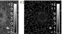
Figure 1.: PSF fitting: a) numerical PSF (star from frame); b) residuals $(GaussianPSF-numericalPSF)/\sqrt{GaussianPSF}$; c) residuals $(filteredPSF-numericalPSF)/\sqrt{filteredPSF}$

3.3. Image reconstruction for QSO 2237+0305

Working with CCD-frames one has a pixel grid naturally introduced in the image frame and deals with discrete functions in (1). So it is necessary to consider the finite difference approximation of the smoothing function:

$$M^{\alpha}[a_{k},g_{ij}]=\sum_{p,q=1}^{N}\frac{1}{\sigma_{pq}^{2}}\left\{\sum_{i,j=1}^{N}\left\{t_{p-i,q-j}\left(\sum_{k=1}^{4}a_{k}\delta_{i-b_{k},j-c_{k}}+g_{ij}\right)\right\}-u_{pq}\right\}^{2}+\alpha\Omega[g_{ij}]$$ (12)

Here the variables are the coordinates and the intensities of the quasar components and the pixel values of the background galaxy.

Image reconstruction on $L_{2}$

The regularization on $L_{2}$ set of functions represents the simplest sort of Tikhonov’s method. Written for the pixel grid the stabilizer:

$$\Omega[\hat{g}_{ij}]=\sum\limits_{i,j=1}^{N}\hat{g}_{ij}^{2}$$ (13)

Here $\hat{g}=g-g_{sersic}$. The parameters of the Sersic model were obtained at preliminary stage using the least-squares method. For the minimization of the smoothing function (12) the conjugate-gradient method was used. Figure 2 shows the results of the image reconstruction. The map of residuals was calculated as follows: $(model_{ij}-cross_{ij})/{\sigma_{ij}}$. Figure 3 shows the astrometry results.

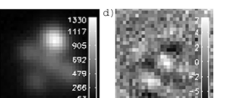
Figure 2.: Reconstruction on $L_{2}$: a) Einstein Cross data; b) solution on $L_{2}$ (logarithmic scale); c) solution convolved with PSF; d) residuals

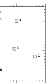
Figure 3.: Astrometry for $L_{2}$-reconstruction

Image reconstruction on $W_{22}$

The discrete expression for the stabilizer is:

$$\begin{array}[]{c}\Omega[\hat{g}_{ij}]=\sum\limits_{i,j=1}^{N}\hat{g}_{ij}^{2}+\sum\limits_{i=2}^{N-1}\sum\limits_{j=1}^{N}(\hat{g}_{i+1,j}-2\hat{g}_{i,j}+\hat{g}_{i-1,j})^{2}+\\ \\ \sum\limits_{i=1}^{N-1}\sum\limits_{j=1}^{N-1}2(\hat{g}_{i+1,j+1}-\hat{g}_{i+1,j}-\hat{g}_{i,j+1}+\hat{g}_{i,j})^{2}+\sum\limits_{i=1}^{N}\sum\limits_{j=2}^{N-1}(\hat{g}_{i,j+1}-2\hat{g}_{i,j}+\hat{g}_{i,j-1})^{2}\end{array}$$

Figure 4 shows the results of the image reconstruction with the regularizing algorithm based on the $W_{22}$ set of functions.

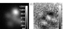
Figure 4.: Reconstruction on $W_{22}$: a) the Einstein Cross data; b) solution on $W_{22}$ (logarithmic scale); c) solution convolved with PSF; d) residuals

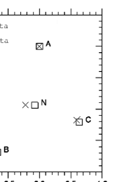
Figure 5.: Astrometry for $W_{22}$-reconstruction

Image reconstruction on $\nu[B]$

The regularization technique with the use of bounded total variation functions is applicable if there are reasons to assume that the unknown solution has discontinuities or rapid variations. The discrete expression for stabilizer reads:

$$\Omega[z]=\sum_{i,j=1}^{N-1}f_{\epsilon}(g_{i+1,j+1}-g_{i+1,j}-g_{i,j+1}+g_{i,j})$$

where $f_{\epsilon}(t)=\sqrt{t^{2}+\left(\frac{\epsilon}{N^{2}}\right)}$. The results of the image restoration are presented on Figure 6.

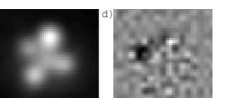
Figure 6.: Reconstruction on the $\nu[B]$: a) Einstein Cross data; b) solution on $\nu[B]$; c) solution convolved with PSF; d) residuals

4. Conclusions

The application of the Tikhonov regularization to the image reconstruction of gravitational lens systems seems to be an effective way of tackling some of the common problems shared by conventional deconvolution algorithms. We have considered several modifications of the regularization method. The illustrative example of the Einstein Cross lens system was used to compare different versions of the algorithm. Although the results look quite encouraging the further work needs to be done to select the appropriate stabilizer function and to produce the pipe-line version of the software.

Acknowledgments.

The work was partially supported by the Russian Foundation for Basic Research (grants 02-01-00044 and 01-02-16800).

References

Belokurov, V.A., Shimanovskaya, E.V., Sazhin, M.V., Yagola, A.G., Artamonov, B.P., Shalyapin, V.N. & Khamitov, I. 2001, Astronomy Reports, 45, 759 (Translated from Astronomicheskii Zhurnal, 78, 876)

Leonov, A.S. 1999. Siberian Journal of Numerical Mathematics, 2, 257

Magain, P., Courbin, F. & Sohy, S. 1998 ApJ, 494, 472

Tikhonov, A.N., Goncharsky, A.V., Stepanov, V.V. & Yagola, A.G. 1995, Numerical methods for the solution of ill-posed problems (Dordrecht: Kluwer Academic Press)

Yagola, A. & Dorofeev, K. 2000 in Fields Institute Communications Vol. 25, Operator Theory and Its Applications, ed. A. G. Ramm, P. N. Shivakumar & A. V. Strauss (Providence, RI: American Mathematical Society), 543