cosmological density fluctuations and gravity waves: a covariant approach to gauge-invariant non-linear perturbation theory

Abstract

We present a new approach to gauge-invariant cosmological perturbations at second order, which is also covariant. We examine two cases in particular for a dust Friedman-Lemaître-Robertson-Walker model of any curvature: we investigate gravity waves generated from clustering matter, that is, induced tensor modes from scalar modes; and we discuss the generation of density fluctuations induced by gravity waves – scalar modes from tensor perturbations. We derive a linear system of evolution equations for second-order gauge-invariant variables which characterise fully the induced modes of interest, with a source formed from variables quadratic in first-order quantities; these we transform into fully-fledged second-order gauge-invariant variables. Both the invariantly defined variables and the key evolution equations are considerably simpler than similar gauge-invariant results derived by other methods. By finding analytical solutions, we demonstrate that non-linear effects can significantly amplify or dampen modes present in standard linearised cosmological perturbation theory, thereby providing an important source of potential error in, and refinement of, the standard model. Moreover, these effects can dominate at late times, and on super-Hubble scales.

I introduction

The standard model of cosmology is built using perturbations of the homogeneous and isotropic Friedman-Lemaître-Robertson-Walker (FLRW) models. These perturbations have, with a few exceptions, been limited to first-order thus far; at first-order, the generic large-scale features of the universe can be accounted for. However, there are good reasons for investigating higher-order perturbations as a refinement of the accuracy of this model. The unprecedented precision of present and upcoming cosmic microwave background (CMB) measurements, such as WMAP and Planck, are reaching levels where non-linear effects may play an important role, especially in any non-Gaussianity present. Indeed, it is rapidly becoming an important area of research to try to predict possible imprints of quantum gravity effects in the CMB; but this can only properly succeed if we also fully understand the range of classical non-linear effects which may produce very similar fluctuations. Non-linear effects may also play an important role in inflation as in the stochastic approach to inflation, which partly includes second-order back-reaction effects GLMM , and also from a fully second-order approach ABMR2 .

Another reason to consider second-order perturbations is that there is no way, within linear theory, to decide when the perturbations have become too large for the theory to handle – i.e., when non-linearities should be taken into account. The reason is that, while it would seem sensible to compare the magnitudes of linearised objects to some invariant background variable, such as the energy density, say, this does not always work, a simple example being gravitational waves in flat space. The study of cosmology is not yet at an advanced enough stage for fully non-linear numerical predictions, as is the case for many astrophysical situations, so second-order perturbation theory is the tool which must be developed for this.

For these reasons, second-order cosmological perturbation theory is beginning to be investigated, following work in the sixties by Tomita tomita who first investigated the second-order terms from scalar modes. For example, other authors have considered second-order perturbations of a flat dust FLRW models, both with MTB and without MMB a cosmological constant. Inflation has also been considered at second order ABMR2 , providing the prediction of the bispectrum of perturbations from inflation. Meanwhile, the evolution of the curvature perturbation on super-Hubble scales after inflation has been shown to be constant at second order MW ; BCLM . More recently, it has been shown that second-order effects can lead to detectable non-Gaussianity in the CMB BMR1 ; BMR2 , as well as polarization MHM . In this paper we complement these results by demonstrating that second-order effects can dominate at late times and on super-Hubble scales over first-order modes.

A crucial aspect of relativistic perturbation theory is the mapping, or gauge choice, between the (fictitious) background and the perturbed spacetime; many perturbation approaches are not invariant with respect to this mapping (see SW ; BS for a comprehensive discussion of this). In terms of coordinates, objects are typically not invariant under infinitesimal coordinate changes. This means that objects and modes specified in one gauge do not always correspond to objects and modes in another, making the interpretation of variables, and the physical situation, difficult. In fact, a gauge-dependent object is not observable BS , which follows from the principle of general covariance. It is therefore important to have a method of describing perturbations using variables which are invariant under gauge transformations. A gauge-invariant object at first-order is a quantity which vanishes (or is constant) in the background; this is the Stewart-Walker Lemma SW . This gauge problem was first solved in cosmology by Bardeen bardeen by providing a full set of gauge-invariant quantities with which to describe the perturbed spacetime. Bardeen’s variables are formed from gauge-invariant (GI) linear combinations of gauge-dependent variables, given in a particular coordinate system; but this prescription can make their interpretation difficult.

This situation has been clarified more recently by the covariant and gauge-invariant perturbation approach of Ellis, Bruni, and others EB ; BDE , using the covariant 1+3 approach EvE . Its strength in cosmological applications lies in the fact that it is well adapted to the system it is describing: all essential information can be captured in a set of (1+3) covariant variables (defined with respect to a preferred timelike observer congruence $u^{a}$), that have an immediate physical and geometrical significance. These variables satisfy a set of evolution and constraint equations, derived from Einstein’s field equations, and the Bianchi and Ricci identities, which form a closed system of equations when an equation of state for the matter is chosen. The covariant and gauge-invariant linearisation procedure is easy and transparent: it consists of deciding which variables are ‘first order’ (or ‘of order $\epsilon$’) and those which are ‘zeroth order’ – i.e., those which do not vanish in the background, which is usually a FLRW model. Products of first-order quantities can then be ignored in the equations. The key point of the approach is that it deals with physically or geometrically relevant quantities, such as the fractional density gradient, ${\cal D}_{a}=a{\mathrm{D}}_{a}\mu/\mu$ (where $a$ is the scale factor, $\mu$ is the gauge-dependent energy density in the perturbed spacetime, and ${\mathrm{D}}_{a}$ is the derivative operator in the observers’ rest space), and the comoving spatial expansion gradient ${\cal Z}_{a}=a{\mathrm{D}}_{a}\theta$ (where $\theta$ is the gauge-dependent expansion), being the most important for scalar perturbations, while the electric and magnetic parts of the Weyl tensor, $E_{ab}$ and $H_{ab}$, respectively, represent the non-local parts of the gravitational field, and describe, amongst other things, the propagation of gravitational waves. All 3-vectors and projected, symmetric, trace-free tensors in this approach, are automatically GI because of the symmetry of the background.

The gauge problem at second-order is quite a challenge: gauge transformations at second-order for second-order variables are huge in general – often as complicated as the evolution equations themselves (see e.g., MMB ; BS ; ABMR2 ). This is a problem far greater than in linear theory in terms of extracting the physics of non-linear effects, simply because it is far harder to intuit the physics by considering a selection of different gauges; the equations are just too complicated, and the range of possible gauges vast. So even choosing a specific gauge at first and second order, one has no guarantee that one has fully understood the problem. The key problem is that for an object to be gauge-invariant at second-order it must vanish in the background and at first-order (or be constant) BS . This problem has hints of a solution in the recent work of Nakamura nakamura , using the methods given in BS , in which a general formalism for deriving GI quantities at second-order, assuming the existence of a method at first-order, is given. Thus it is possible that a fully gauge-invariant second-order theory may be presented in the near future using Bardeen’s method for constructing first-order GI quantities together with Nakamura’s approach. There has been recent progress along these lines; ABMR2 have given a gauge-invariant definition of the comoving curvature at second-order for scalar perturbations. Nevertheless, it is likely that when such a theory is found it will be very difficult to understand exactly what everything means, especially as the construction is not unique, although it will likely be crucial for numerical prediction of observable quantities such as the CMB power spectrum.

In this paper we discuss an alternative route to second-order gauge-invariant perturbations in cosmology following the covariant route initiated in EB . The covariant 1+3 approach is a good method for perturbation theory simply because it is manifestly covariant; many of the usual gauge-problems arise as a result of coordinate transformations at each order. Once we have a complete set of GI variables, then we know that they are observable BS , and correspond to physical or geometrical quantities.

Using a zeroth-order background of a dust FLRW model with zero cosmological constant, we discuss ‘mode-crossing’ perturbations; that is, perturbations at second order generated from an ‘orthogonal mode’ at first order – second-order tensor modes generated by first-order scalar modes (Section III.1), and viceversa (Section III.2). We define a complete set of second-order gauge-invariant quantities which fully describe the induced modes, and convert all products of first-order quantities appearing in the second-order equations into new second-order variables, thus making the equations explicitly GI at second order, in a manner very similar to CMBD . This simplifies the presentation of the equations by converting them into a linear system of DE’s, a procedure which also simplifies their solution. In the case of first-order tensor modes, this system is infinite dimensional reflecting the coupling of modes of each wavelength feeding into the induced scalar modes. The standard zeroth-order harmonic functions can be used on second-order variables to remove the tensorial nature of the equations, and remove spatial gradients so converting the system into odes which may then be easily integrated. We explicitly integrate both cases under investigation to show that scalar-mode coupling effects may play an important role at both early and late times, and on small and large scales.

II first-order perturbation: the covariant formulation

The 1+3 approach relies upon the introduction of a family of observers travelling on a four-velocity $u^{a}$, with which all geometrical and physical objects and operators – essentially the Riemann curvature tensor and the covariant derivative – are decomposed into invariant parts; scalars along $u^{a}$ and scalars, 3-vectors, and projected, symmetric and trace-free (PSTF) tensors orthogonal to $u^{a}$, as well as an evolution derivative along $u^{a}$ and a spatial derivative orthogonal to it. The Einstein field equations are supplemented by the Ricci identities for $u^{a}$ and the Bianchi identities, forming an complete set of first-order differential equations. We refer to EvE for details and references; we also follow their notation and sign conventions.

Perturbations at first-order around a FLRW background are relatively straightforward: define the first-order gauge-invariant (FOGI) variables corresponding to the spatial fluctuations in the energy density and expansion:

$$X_{a} = {\mathrm{D}}_{a}\mu,$$ (1)

$$Z_{a} = {\mathrm{D}}_{a}\theta.$$ (2)

These are FOGI simply because they vanish in the exact FLRW background SW ; BS . We shall not use the more physically motivated variables ${\cal D}_{a}=a{\mathrm{D}}_{a}\mu/\mu$ and ${\cal Z}_{a}=a{\mathrm{D}}_{a}\theta$, as these tend to make the equations more complicated to derive at second-order. Ignoring rotational perturbations the set of FOGI equations consists of the evolution equations

$$\dot{X}_{a} = -{\textstyle\frac{4}{3}}\theta X_{a}-\mu Z_{a},$$ (3)

$$\dot{Z}_{a} = -\theta Z_{a}-{\textstyle\frac{1}{2}}X_{a},$$ (4)

$$\dot{\sigma}_{ab} = -{\textstyle\frac{2}{3}}\theta\sigma_{ab}-E_{ab},$$ (5)

$$\dot{E}_{ab}-\hskip 0.9pt{\mathsf{curl}\hskip 2.0pt}H_{ab} = -{\textstyle\frac{1}{2}}\mu\sigma_{ab}-\theta E_{ab},$$ (6)

$$\dot{H}_{ab}+\hskip 0.9pt{\mathsf{curl}\hskip 2.0pt}E_{ab} = -\theta H_{ab};$$ (7)

and the constraints

$$0 = {\textstyle\frac{1}{3}}X_{a}-\hskip 0.9pt{\mathsf{div}\hskip 2.0pt}E_{a},$$ (8)

$$0 = {\textstyle\frac{2}{3}}Z_{a}-\hskip 0.9pt{\mathsf{div}\hskip 2.0pt}\sigma_{a},$$ (9)

$$0 = \hskip 0.9pt{\mathsf{div}\hskip 2.0pt}H_{a},$$ (10)

$$0 = H_{ab}-\hskip 0.9pt{\mathsf{curl}\hskip 2.0pt}\sigma_{ab},$$ (11)

$$0 = \hskip 0.9pt{\mathsf{curl}\hskip 2.0pt}X_{a},$$ (12)

$$0 = \hskip 0.9pt{\mathsf{curl}\hskip 2.0pt}Z_{a}.$$ (13)

The whole system of equations is governed entirely by the shear, which obeys the covariant wave-like equation:

$$\ddot{\sigma}_{ab}+\hskip 0.9pt{\mathsf{curl}\hskip 2.0pt}\hskip 0.9pt{\mathsf{curl}\hskip 2.0pt}\sigma_{ab}+{\textstyle\frac{5}{3}}\theta\dot{\sigma}_{ab}+\left({\textstyle\frac{4}{9}}\theta^{2}-{\textstyle\frac{5}{6}}\mu\right)\sigma_{ab}=0.$$ (14)

Each other object is determined by solutions of this equation – no further integration of the equations is required after the solution for the shear is found. Indeed it is useful to use $\{\sigma_{ab},\dot{\sigma}_{ab}\}$ as the ‘basis vector’ for the full solution, as we shall do later. While each variable in the problem may be shown to satisfy a wave-like equation of some sort, these do not necessarily close; in particular, the wave equation for $E_{ab}$ in the case of gravity wave propagation has a source term from the shear chal ; DBE .

Because the background is homogeneous and isotropic, each FOGI vector may be uniquely split into a curl-free and divergence-free part, usually referred to as scalar and vector parts respectively, which we write as

$$V_{a}={V_{\hskip-0.8pt\mathrel{\vbox{\hbox{\tiny\ooalign{\raise 1.5pt\hbox{{S}}}}}}}}_{a}+{V_{\hskip-0.8pt\mathrel{\vbox{\hbox{\tiny\ooalign{\raise 1.5pt\hbox{{V}}}}}}}}_{a}~{}~{}~{}\mbox{where}~{}~{}~{}\hskip 0.9pt{\mathsf{curl}\hskip 2.0pt}{V_{\hskip-0.8pt\mathrel{\vbox{\hbox{\tiny\ooalign{\raise 1.5pt\hbox{{S}}}}}}}}_{a}=0~{}~{}~{}\mbox{and}~{}~{}~{}\hskip 0.9pt{\mathsf{div}\hskip 2.0pt}{V_{\hskip-0.8pt\mathrel{\vbox{\hbox{\tiny\ooalign{\raise 1.5pt\hbox{{V}}}}}}}}=0.$$ (15)

Similarly, any tensor may be invariantly split into scalar, vector and tensor parts:

$$T_{ab}={T_{\hskip-0.8pt\mathrel{\vbox{\hbox{\tiny\ooalign{\raise 1.5pt\hbox{{S}}}}}}}}_{ab}+{T_{\hskip-0.8pt\mathrel{\vbox{\hbox{\tiny\ooalign{\raise 1.5pt\hbox{{V}}}}}}}}_{ab}+{T_{\hskip-0.8pt\mathrel{\vbox{\hbox{\tiny\ooalign{\raise 1.5pt\hbox{{T}}}}}}}}_{ab}~{}~{}~{}\mbox{where}~{}~{}~{}\hskip 0.9pt{\mathsf{curl}\hskip 2.0pt}{T_{\hskip-0.8pt\mathrel{\vbox{\hbox{\tiny\ooalign{\raise 1.5pt\hbox{{S}}}}}}}}_{ab}=0,~{}~{}~{}\hskip 0.9pt{\mathsf{div}\hskip 2.0pt}\hskip 0.9pt{\mathsf{div}\hskip 2.0pt}{T_{\hskip-0.8pt\mathrel{\vbox{\hbox{\tiny\ooalign{\raise 1.5pt\hbox{{V}}}}}}}}=0,~{}~{}~{}\mbox{and}~{}~{}~{}\hskip 0.9pt{\mathsf{div}\hskip 2.0pt}{T_{\hskip-0.8pt\mathrel{\vbox{\hbox{\tiny\ooalign{\raise 1.5pt\hbox{{T}}}}}}}}_{a}=0.$$ (16)

In the equations we can separately equate scalar, vector and tensor parts. As we are ignoring rotation, all vector parts are zero.

Each FOGI vector consists of only the scalar part and is curl-free; so

$$X^{a}={X_{\hskip-0.8pt\mathrel{\vbox{\hbox{\tiny\ooalign{\raise 1.5pt\hbox{{S}}}}}}}}^{a},$$ (17)

similarly for $Z^{a}$. Each tensor consists of a scalar and a tensor part, which describe clustering matter and gravity waves respectively. Thus the equations can still be manipulated further: splitting the shear into its curl free and divergence free parts gives us an oscillatory equation for the scalar part, which tells us the increase in shear found as matter clusters:

$$\ddot{\sigma_{\hskip-0.8pt\mathrel{\vbox{\hbox{\tiny\ooalign{\raise 1.5pt\hbox{{S}}}}}}}}_{ab}+{\textstyle\frac{5}{3}}\theta\dot{\sigma_{\hskip-0.8pt\mathrel{\vbox{\hbox{\tiny\ooalign{\raise 1.5pt\hbox{{S}}}}}}}}_{ab}+\left({\textstyle\frac{4}{9}}\theta^{2}-{\textstyle\frac{5}{6}}\mu\right){\sigma_{\hskip-0.8pt\mathrel{\vbox{\hbox{\tiny\ooalign{\raise 1.5pt\hbox{{S}}}}}}}}_{ab}=0,$$ (18)

and a wave equation for the tensor part, which is the equation governing gravity waves in an expanding dust universe:

$$\ddot{\sigma_{\hskip-0.8pt\mathrel{\vbox{\hbox{\tiny\ooalign{\raise 1.5pt\hbox{{T}}}}}}}}_{ab}-{\mathrm{D}}^{2}{\sigma_{\hskip-0.8pt\mathrel{\vbox{\hbox{\tiny\ooalign{\raise 1.5pt\hbox{{T}}}}}}}}_{ab}+{\textstyle\frac{5}{3}}\theta\dot{\sigma_{\hskip-0.8pt\mathrel{\vbox{\hbox{\tiny\ooalign{\raise 1.5pt\hbox{{T}}}}}}}}_{ab}+\left({\textstyle\frac{1}{9}}\theta^{2}+{\textstyle\frac{1}{6}}\mu\right){\sigma_{\hskip-0.8pt\mathrel{\vbox{\hbox{\tiny\ooalign{\raise 1.5pt\hbox{{T}}}}}}}}_{ab}=0,$$ (19)

which may be shown using the identity for a FOGI tensor:

$$\hskip 0.9pt{\mathsf{curl}\hskip 2.0pt}\hskip 0.9pt{\mathsf{curl}\hskip 2.0pt}T_{ab}=-{\mathrm{D}}^{2}T_{ab}+{\textstyle\frac{3}{2}}{\mathrm{D}}_{\langle a}\hskip 0.9pt{\mathsf{div}\hskip 2.0pt}T_{b\rangle}+\left(\mu-{\textstyle\frac{1}{3}}\theta^{2}\right)T_{ab}.$$ (20)

The other two tensors can be similarly split. Because the magnetic Weyl curvature is the curl of the shear, the scalar part of it vanishes at this order.

We shall use Eqs. (18) and (19) to form the source for second-order perturbations.

III second-order perturbation

Lets consider non-linear perturbations up to second order in the shear, ignoring rotation and fluid modes at both first and second order, but keeping both scalar and tensor modes. The shear ‘wave’ equation becomes

$$\ddot{\sigma}_{ab}+\hskip 0.9pt{\mathsf{curl}\hskip 2.0pt}\hskip 0.9pt{\mathsf{curl}\hskip 2.0pt}\sigma_{ab}+{\textstyle\frac{5}{3}}\theta\dot{\sigma}_{ab}+\left({\textstyle\frac{4}{9}}\theta^{2}-{\textstyle\frac{5}{6}}\mu\right)\sigma_{ab}=\sigma_{c\langle a}\dot{\sigma}_{b\rangle}^{~{}~{}c}+\theta\sigma_{c\langle a}\sigma_{b\rangle}^{~{}~{}c},$$ (21)

where the ‘curl-curl’ operator now has the quadratic contributions when converting to the Laplacian:

$$\hskip 0.9pt{\mathsf{curl}\hskip 2.0pt}\hskip 0.9pt{\mathsf{curl}\hskip 2.0pt}T_{ab}=-{\mathrm{D}}^{2}T_{ab}+{\textstyle\frac{3}{2}}{\mathrm{D}}_{\langle a}\hskip 0.9pt{\mathsf{div}\hskip 2.0pt}T_{b\rangle}+\left(\mu-{\textstyle\frac{1}{3}}\theta^{2}\right)T_{ab}+3E_{c\langle a}T_{b\rangle}^{~{}~{}c}-\theta\sigma_{c\langle a}T_{b\rangle}^{~{}~{}c}.$$ (22)

In deriving Eq. (21) we have substituted for the Weyl curvature in terms of the shear, given by Eqs. (5) and (11). We have neglected terms ${\cal O}(\sigma^{3})$ (and derivatives of), which is a consistent covariant linearisation procedure to second order. There are some important things to note about Eq. (21):

1. It is not actually second order in the usual perturbative sense. The shear appearing in the quadratic shear terms on the rhs should not be the same as that on the left; on the left we have a mixture of first and second-order quantities, but on the right, the terms are made up of products of first-order variables. Integrating Eq. (21) without explicitly taking into account this distinction will give a different solution than explicitly making it so [by using solutions of Eq. (14) for the terms on the right].

2. It is not gauge-invariant. The mixture of first and second-order quantities on the left is really the core of the gauge problem: the ‘first-order bits’ don’t cancel out upon application of Eq. (14) because the derivative operators in each of the two equations are not the same. In the second-order equation there are derivative operators of order one hanging around; but solution of the linear problem does not tell us what these are. Hence, the equation can’t be integrated.

We shall now convert Eq. (21) into a gauge-invariant equation at second order in the two cases we have mentioned.

III.1 GRAVITY WAVES FROM DENSITY FLUCTUATIONS

Consider the case where we excite only the scalar modes at linear order, which describe density perturbations. These modes are covariantly characterised at linear order by the GI condition

$$\hskip 0.9pt{\mathsf{curl}\hskip 2.0pt}\sigma_{ab}=0.$$ (23)

Hence, we may define the variable

$$\Sigma_{ab}=\hskip 0.9pt{\mathsf{curl}\hskip 2.0pt}{\sigma}_{ab}$$ (24)

which is second-order and gauge-invariant up to and including second-order (SOGI), as it vanishes at all lower orders BS ; this variable forms the core of the analysis of gravity waves generated by density fluctuations. In fact, it is just the magnetic part of the Weyl tensor if rotational modes are ignored (as may be seen from the $\hskip 0.9pt{\mathsf{curl}\hskip 2.0pt}\sigma_{ab}$ constraint); nevertheless, it is a distinction worth keeping, as this would not usually be the case. Taking the curl of Eq. (21), or taking the time derivative of the magnetic Weyl evolution equation results in the equation for $\Sigma_{ab}$:

$$\ddot{\Sigma}_{ab}+\hskip 0.9pt{\mathsf{curl}\hskip 2.0pt}\hskip 0.9pt{\mathsf{curl}\hskip 2.0pt}\Sigma_{ab}+{\textstyle\frac{7}{3}}\theta\dot{\Sigma}_{ab}+\left(\theta^{2}-\mu\right)\Sigma_{ab}={\cal S}_{ab}$$ (25)

where the source term is given by

$${\cal S}_{ab} = \epsilon_{cd\langle a}\bigl{\{}-{\textstyle\frac{5}{2}}\dot{\sigma}_{b\rangle}^{~{}~{}d}\hskip 0.9pt{\mathsf{div}\hskip 2.0pt}\sigma^{c}-{\textstyle\frac{5}{2}}\sigma_{b\rangle}^{~{}~{}d}\hskip 0.9pt{\mathsf{div}\hskip 2.0pt}\dot{\sigma}^{c}-{\textstyle\frac{9}{3}}\theta\sigma_{b\rangle}^{~{}~{}d}\hskip 0.9pt{\mathsf{div}\hskip 2.0pt}\sigma^{c}$$ (26)

$$-\dot{\sigma}^{ec}{\mathrm{D}}_{|e|}\sigma_{b\rangle}^{~{}~{}d}-2\sigma^{ec}{\mathrm{D}}_{|e|}\dot{\sigma}_{b\rangle}^{~{}~{}d}+{\textstyle\frac{1}{2}}\sigma^{de}{\mathrm{D}}^{c}\dot{\sigma}_{b\rangle e}+{\textstyle\frac{1}{2}}\dot{\sigma}^{de}{\mathrm{D}}^{c}\sigma_{b\rangle e}$$

$$+{\textstyle\frac{1}{2}}\sigma^{~{}~{}e}_{b\rangle}{\mathrm{D}}^{c}\dot{\sigma}_{e}^{~{}d}+{\textstyle\frac{1}{2}}\dot{\sigma}^{~{}~{}e}_{b\rangle}{\mathrm{D}}^{c}\sigma_{e}^{~{}d}+\theta{\mathrm{D}}^{c}\left(\sigma_{b\rangle e}\sigma^{de}\right)\bigr{\}}.$$

This source term is considerably more untidy than that of the gauge-dependent equation for the shear, Eq. (21) because of the extra terms which arise from successive applications of the commutation relation

$$\left(\hskip 0.9pt{\mathsf{curl}\hskip 2.0pt}T_{ab}\right)^{{}^{\mathbf{{}_{\cdot}}}}-\hskip 0.9pt{\mathsf{curl}\hskip 2.0pt}\dot{T}_{ab}=-{\textstyle\frac{1}{3}}\theta\hskip 0.9pt{\mathsf{curl}\hskip 2.0pt}T_{ab}-\epsilon_{cd\langle a}\sigma^{ec}{\mathrm{D}}_{|e|}T_{b\rangle}^{~{}~{}d},$$ (27)

which holds for this case.

The second-order equation (25) is not yet properly SOGI because the rhs contains terms which are FOGI, although the rhs as a whole is second-order, and ${\cal S}_{ab}$ is a SOGI tensor. To make the source explicitly composed of SOGI quantities, we define the SOGI variables:

$$\psi_{1ab} = \epsilon_{cd\langle a}\left(\hskip 0.9pt{\mathsf{div}\hskip 2.0pt}\sigma^{c}\right)\sigma_{b\rangle}^{~{}~{}d},$$ (28)

$$\psi_{2ab} = \epsilon_{cd\langle a}\left(\hskip 0.9pt{\mathsf{div}\hskip 2.0pt}\sigma^{c}\right)\dot{\sigma}_{b\rangle}^{~{}~{}d},$$ (29)

$$\psi_{3ab} = \epsilon_{cd\langle a}\left(\hskip 0.9pt{\mathsf{div}\hskip 2.0pt}\dot{\sigma}^{c}\right)\sigma_{b\rangle}^{~{}~{}d},$$ (30)

$$\psi_{4ab} = \epsilon_{cd\langle a}\left(\hskip 0.9pt{\mathsf{div}\hskip 2.0pt}\dot{\sigma}^{c}\right)\dot{\sigma}_{b\rangle}^{~{}~{}d};.$$ (31)

It is straightforward to show that, to second order, these variables satisfy the closed system of evolution equations

$$\dot{\mbox{\boldmath$\mathrm{\psi}$}}_{ab}={\mbox{\boldmath$\mathrm{\Psi\psi}$}}_{ab},$$ (32)

where ${\mbox{\boldmath$\mathrm{\psi}$}}_{ab}=\left(\psi_{1ab},\psi_{2ab},\psi_{3ab},\psi_{4ab}\right)$, and the scalar-scalar coupling matrix is given by

$${\mbox{\boldmath$\mathrm{\Psi}$}}=\left(\begin{array}[]{cccc}-{\textstyle\frac{1}{3}}\theta&1&1&0\\ -{\textstyle\frac{4}{9}}\theta^{2}+{\textstyle\frac{5}{6}}\mu{}{}&-2\theta&0&1\\ -{\textstyle\frac{4}{9}}\theta^{2}+{\textstyle\frac{5}{6}}\mu{}{}&0&-2\theta&1\\ 0&-{\textstyle\frac{4}{9}}\theta^{2}+{\textstyle\frac{5}{6}}\mu{}{}&-{\textstyle\frac{4}{9}}\theta^{2}+{\textstyle\frac{5}{6}}\mu{}{}&-{\textstyle\frac{11}{3}}\theta\end{array}\right),$$ (33)

which is derived using Eq. (18). Similarly, we may define the variables

$$\phi_{1ab} = \epsilon_{cd\langle a}(\hskip 0.9pt{\mathsf{dis}\hskip 2.0pt}\sigma^{c}_{~{}b\rangle e})\sigma^{de},$$ (34)

$$\phi_{2ab} = \epsilon_{cd\langle a}(\hskip 0.9pt{\mathsf{dis}\hskip 2.0pt}\sigma^{c}_{~{}b\rangle e})\dot{\sigma}^{de},$$ (35)

$$\phi_{3ab} = \epsilon_{cd\langle a}(\hskip 0.9pt{\mathsf{dis}\hskip 2.0pt}\dot{\sigma}^{c}_{~{}b\rangle e})\sigma^{de},$$ (36)

$$\phi_{4ab} = \epsilon_{cd\langle a}(\hskip 0.9pt{\mathsf{dis}\hskip 2.0pt}\dot{\sigma}^{c}_{~{}b\rangle e})\dot{\sigma}^{de},$$ (37)

where we have defined the distortion of $\sigma_{ab}$ as

$$\hskip 0.9pt{\mathsf{dis}\hskip 2.0pt}\sigma_{cab}={\mathrm{D}}_{\langle c}\sigma_{ab\rangle},$$ (38)

which is the remaining invariantly defined part of the spatial derivative of a PSTF tensor which is not part of the divergence or curl MES . It is clear that these variables, ${\mbox{\boldmath$\mathrm{\phi}$}}_{ab}$, obey the same evolution equation as ${\mbox{\boldmath$\mathrm{\psi}$}}_{ab}$, given by Eq. (32). By performing a complete 1+3 split of the derivatives of the shear in the source of Eq. (25) to write them in terms of the divergence and distortion only, we may write our source term in terms of these SOGI variables:

$${\cal S}_{ab} = -{\textstyle\frac{22}{5}}\theta\psi_{1ab}-{\textstyle\frac{27}{20}}\psi_{2ab}+{\textstyle\frac{3}{20}}\psi_{3ab}+\theta\phi_{1ab}+{\textstyle\frac{3}{2}}\phi_{2ab}+{\textstyle\frac{5}{2}}\phi_{3ab}.$$ (39)

We now have a complete closed linear system of differential equations which may be expanded in the usual background harmonics, and integrated straightforwardly (especially numerically) once initial data is prescribed. By taking various spatial gradients of these eight variables it can be shown that there are some (differential) constraints which must be satisfied amongst these variables, which serve to constrain initial data, but we shall not pursue this further here (see SMEL for details of where these come from). Note that we have managed to deal with all the complicated scalar-scalar coupling without recourse to harmonics.

The mode-mode coupling variables, ${\mbox{\boldmath$\mathrm{\psi}$}}_{ab},{\mbox{\boldmath$\mathrm{\phi}$}}_{ab}$ do several things in aiding the solution to Eq (21) at second-order: they transform Eq. (25) into a genuinely second-order equation in the perturbative sense because in calculating their evolution equations we neglected terms ${\cal O}(\sigma^{3})$, and made the final distinction between the variables on the lhs and those on the right; they turn Eq. (25) into an explicitly SOGI equation consisting only of SOGI variables; and finally they turn the system of equations which must be solved into a system of linear differential equations, which are much easier to integrate numerically, and analyse by other techniques, than systems which are not linear.

III.1.1 the induced tensor modes

The mode coupling which provides the source for the second order perturbation, although being products of scalar mode variables, induces tensor modes at second order (and, in more general situations, rotational modes), seen by the fact that $\hskip 0.9pt{\mathsf{curl}\hskip 2.0pt}{\cal S}_{ab}\neq 0$. This mode-mixing is perhaps one of the most interesting parts of non-linear perturbation theory; as we show here, for example, gravity waves may be generated – or reduced – purely from the effects of linear clustering of matter. The second-order scalar modes which $\Sigma_{ab}$ tells us about, however, are not genuine second order effects: for scalar modes, $\hskip 0.9pt{\mathsf{div}\hskip 2.0pt}\Sigma_{a}\neq 0$, and is in fact just a combination of quadratic first-order variables, as may be seen through the $\hskip 0.9pt{\mathsf{div}\hskip 2.0pt}H_{a}$ constraint. It is interesting to note that

$$\hskip 0.9pt{\mathsf{div}\hskip 2.0pt}\Sigma_{a}=\epsilon_{abc}\sigma^{bd}\dot{\sigma}^{c}_{~{}d}=\sum_{k,k^{\prime}}\sigma_{(k)}\dot{\sigma}_{(k^{\prime})}\underbrace{\epsilon_{abc}Q_{(k)}^{bd}{Q_{(k^{\prime})}}^{c}_{~{}d}}_{=0~{}\mbox{when}~{}k=k^{\prime}},$$ (40)

using standard harmonics chal ; EvE , so coupling between modes of differing wavelength do not give rise to tensor modes at second order, for which $\hskip 0.9pt{\mathsf{div}\hskip 2.0pt}\Sigma_{a}=0=\hskip 0.9pt{\mathsf{div}\hskip 2.0pt}H_{a}$. This is a reflection of the integrability conditions discussed in SMEL , which suggests that $\hskip 0.9pt{\mathsf{div}\hskip 2.0pt}H_{a}=0$ may not be as restrictive in perturbative models as it is in the fully non-linear case.

The second order tensor modes, on the other hand, are covariantly characterised by $\hskip 0.9pt{\mathsf{div}\hskip 2.0pt}\Sigma_{a}=0$, for which we have the genuine wave equation:

$${{{\ddot{\Sigma}}{{}_{\hskip-0.8pt\mathrel{\vbox{\hbox{\tiny\ooalign{\raise 1.5pt\hbox{{T}}}}}}}}}}_{ab}-{\mathrm{D}}^{2}{\Sigma_{\hskip-0.8pt\mathrel{\vbox{\hbox{\tiny\ooalign{\raise 1.5pt\hbox{{T}}}}}}}}_{ab}+{\textstyle\frac{7}{3}}\theta{\dot{\Sigma}{{}_{\hskip-0.8pt\mathrel{\vbox{\hbox{\tiny\ooalign{\raise 1.5pt\hbox{{T}}}}}}}}}_{ab}+{{\textstyle\frac{2}{3}}\theta^{2}}{\Sigma_{\hskip-0.8pt\mathrel{\vbox{\hbox{\tiny\ooalign{\raise 1.5pt\hbox{{T}}}}}}}}_{ab}={\cal S}{{}_{\hskip-0.8pt\mathrel{\vbox{\hbox{\tiny\ooalign{\raise 1.5pt\hbox{{T}}}}}}}}_{ab},$$ (41)

upon using Eq. (22) in Eq. (25). Harmonic functions, defined as usual in the background (any changes would be ${\cal O}(3)$), may now be introduced, and the equations integrated in time; we discuss this in the case of a flat background below.

Now, gravity waves are waves in the Weyl curvature which induce waves in the shear (non-local waves which travel at the speed of light and thus can’t be removed by a change of observers), so in order to fully understand gravitational radiation induced by density fluctuations, we must relate $\Sigma_{ab}$ to the Weyl curvature. This simply involves creating SOGI variables for the Weyl curvature. The magnetic part is easy, as we have $H_{ab}=\Sigma_{ab}$ in the absence of rotation, while for the electric part of the Weyl tensor we may define

$$\mathscr{E}_{ab}=\hskip 0.9pt{\mathsf{curl}\hskip 2.0pt}E_{ab}=-\dot{\Sigma}_{ab}-\theta\Sigma_{ab}+{\textstyle\frac{6}{5}}\psi_{1ab},$$ (42)

which completes the solution for the induced tensor modes.

In the case of a flat background, the equations are particularly easy to integrate (see chal for details on solving the homogeneous part of Eq. (41) in a non-flat background): we have the scale factor $a=a_{0}t^{2/3}$ (we set $a_{0}=1$), implying $\theta=2/t$ and $\mu={\textstyle\frac{1}{3}}\theta^{2}$; integrating Eq. (32) for ${\mbox{\boldmath$\mathrm{\psi}$}}_{ab}$ and ${\mbox{\boldmath$\mathrm{\phi}$}}_{ab}$, we find that the source has three components:

$${\cal S}_{ab}=\alpha_{ab}t^{-7/3}+\beta_{ab}t^{-4}+\gamma_{ab}t^{-17/3},$$ (43)

where the last term is the largest at early times (which has the time dependence of $a^{-1}\sigma\dot{\sigma}$). The tensors $\alpha_{ab},~{}\beta_{ab}$ and $\gamma_{ab}$ are constant in time and are a combination of the initial conditions of ${\mbox{\boldmath$\mathrm{\psi}$}}_{ab}$ and ${\mbox{\boldmath$\mathrm{\phi}$}}_{ab}$; the details of this need not concern us here. Using standard tensor harmonics BDE ; chal removes the tensorial nature and spatial dependence of the wave equation (41), and replaces the covariant Laplacian with a harmonic index, ${\mathrm{D}}^{2}\mapsto-k^{2}/a^{2}$, the full solution being a sum over harmonic modes. The analytic solution to Eq. (41) may be easily obtained:

$$\Sigma^{(k)}=\Sigma_{1}^{(k)}+\Sigma_{2}^{(k)}+\alpha^{(k)}k^{-2}t^{-1}+\beta^{(k)}k^{-2}t^{-8/3}+\gamma^{(k)}\times{\mbox{mess}}$$ (44)

where the two solutions to the homogeneous part are

$$\Sigma_{1}^{(k)} = S_{1}^{(k)}t^{-8/3}\left[\left(3x^{2}-1\right)\cos 3x-3x\sin 3x\right]$$ (45)

$$\Sigma_{2}^{(k)} = S_{2}^{(k)}t^{-8/3}\left[\left(3x^{2}-1\right)\sin 3x+3x\cos 3x\right]$$ (46)

where $x=kt^{1/3}$ and $S_{1}^{(k)},S_{2}^{(k)}$ are constants. The ‘mess’ from the $\gamma_{ab}$ term dominates the solution at early times and on super-Hubble scales, when $t\ll 1$ and $x\ll 1$ respectively:

$$\Sigma^{(k)}\sim{\textstyle\frac{3}{8}}\gamma^{(k)}t^{-11/3}\left[1-{\textstyle\frac{3}{4}}x\right]+{\cal O}({t^{-8/3}}),$$ (47)

with the next term arising from the homogeneous solution. Meanwhile, at late times we have a new power law behaviour dominating from the scalar mode interaction

$$\Sigma^{(k)}\sim k^{-2}\alpha^{(k)}t^{-1}+3k^{2}t^{-2}\left\{S_{2}^{(k)}\sin 3x-\left(S_{1}+{\textstyle\frac{81}{256}}k^{3}\pi\gamma^{(k)}\right)\cos 3x\right\}+{\cal O}(t^{-7/3}),$$ (48)

while we see that on small scales ($k\gg 1$) at late times the oscillatory behaviour is also dominated by the scalar mode interaction. Thus, in many regions of interest the terms arising from the scalar mode coupling dominate the solution.

In Fig. 1 we show some solution curves for $\Sigma^{(k)}$ for a flat model both with and without the non-linear source. This shows that the effect of including the scalar-scalar interaction in the generation of gravity waves may increase or decrease the amplitude and power of the induced tensor perturbations for a given wavelength, possibly quite significantly. This may have implications for the spectrum of tensor modes in the cosmic microwave background (see e.g., chal ; MM97 for details of calculating the CMB power spectrum from the solutions given here).

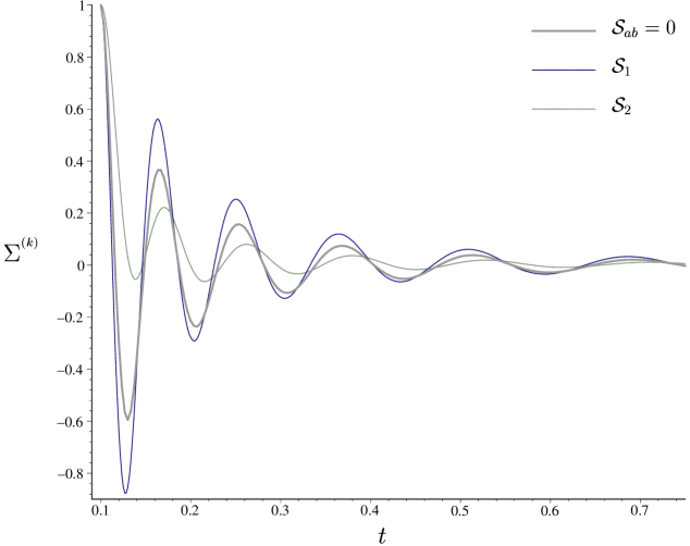
Figure 1: The induced gravity waves from non-linear density fluctuations for a flat background. Here we have shown the harmonic component of $\Sigma_{ab}$, $\Sigma^{(k)}$, corresponding to $k/a_{0}=25$ in three situations, all of which have initial conditions such that $\Sigma^{(k)}=1$ and $\dot{\Sigma}^{(k)}=0$ at $t=0.1$ (in arbitrary units). The thick grey curve represents the oscillatory decay of gravity waves with no source present, as predicted from linear theory. To contrast with that we have shown two different cases: curve ${\cal S}_{1}$ has parameters from the source term $\alpha^{(k)}=0,~{}\beta^{(k)}=0.8,~{}\gamma^{(k)}=-.03$, which shows considerable amplification of the gravity waves over the linear case, while curve ${\cal S}_{2}$ has $\alpha^{(k)}=1,~{}\beta^{(k)}=0,~{}\gamma^{(k)}=.02$, which shows significant damping.

III.2 DENSITY FLUCTUATIONS FROM GRAVITY WAVES

We shall now look at the reverse situation from the previous section, and consider the case where only tensor perturbations are excited at first order. To second order we shall still neglect rotation and fluid modes for simplicity of exposition, and study the induced density fluctuations, characterised by the scalar modes.

Pure tensor modes are covariantly characterised by the FOGI condition

$$\hskip 0.9pt{\mathsf{div}\hskip 2.0pt}\sigma_{a}=0$$ (49)

from which it follows that the divergence of the two Weyl curvature tensors must vanish also. Thus, at second order, we use the SOGI variable

$$\Delta_{a}=\hskip 0.9pt{\mathsf{div}\hskip 2.0pt}\sigma_{a}$$ (50)

as our key variable. From the $\hskip 0.9pt{\mathsf{div}\hskip 2.0pt}H_{a}$-constraint and the non-linear commutation relation

$$\hskip 0.9pt{\mathsf{div}\hskip 2.0pt}\hskip 0.9pt{\mathsf{curl}\hskip 2.0pt}T_{a}-{\textstyle\frac{1}{2}}\hskip 0.9pt{\mathsf{curl}\hskip 2.0pt}\hskip 0.9pt{\mathsf{div}\hskip 2.0pt}T_{a}=\epsilon_{abc}E^{bd}T^{c}_{~{}d}-{\textstyle\frac{1}{3}}\theta\epsilon_{abc}\sigma^{bd}T^{c}_{~{}d},$$ (51)

we find that $\hskip 0.9pt{\mathsf{curl}\hskip 2.0pt}\Delta_{a}=0$ because we’re ignoring rotation – so $\Delta_{a}$ contains only scalar modes. Our wave-like equation for $\sigma_{ab}$, Eq. (25), becomes, upon taking its divergence,

$$\ddot{\Delta}_{a}+{\textstyle\frac{7}{3}}\theta\dot{\Delta}_{a}+\left(\theta^{2}-\mu\right)\Delta_{a}={\cal T}_{a}$$ (52)

where the source arising from tensor-tensor coupling is, neglecting terms ${\cal O}(\sigma^{3})$ and ${\cal O}(\sigma\times\Delta)$,

$${\cal T}_{a}=-{\textstyle\frac{2}{3}}\theta{\mathrm{D}}_{a}\left(\sigma^{bc}\sigma_{bc}\right)-{\textstyle\frac{4}{3}}{\mathrm{D}}_{a}\left(\sigma_{bc}\dot{\sigma}^{bc}\right),$$ (53)

which is remarkably simple, despite several applications of the commutation relation Eq. (51) and

$$\left(\hskip 0.9pt{\mathsf{div}\hskip 2.0pt}T_{a}\right)^{{}^{\mathbf{{}_{\cdot}}}}-\hskip 0.9pt{\mathsf{div}\hskip 2.0pt}\dot{T}_{a}=-{\textstyle\frac{1}{3}}\theta\hskip 0.9pt{\mathsf{div}\hskip 2.0pt}T_{a}-\sigma^{bc}{\mathrm{D}}_{b}T_{ac}+\epsilon_{abc}H^{bd}T^{c}_{~{}d}.$$ (54)

We have again substituted for the Weyl curvature in terms of the shear.

As in the previous case, we may make the source for Eq. (52) explicitly SOGI by introducing a set of SOGI variables; variables which are constructed from quadratic FOGI variables. However, the presence of the Laplacian in the wave equation for the tensor modes at first-order means that we need an infinite set of these variables; a mode of one particular wavelength at first-order couples with all higher wavelength modes at second order. One can approach this in two ways: explicitly split the first-order solution into a sum over tensor harmonics; when inserted into the source term ${\cal T}_{a}$ we have an infinite sum (over $k$ and $k^{\prime}$) over terms of the form $\sigma^{(k)}\sigma^{(k^{\prime})}Q_{\hskip-0.8pt\mathrel{\vbox{\hbox{\tiny\ooalign{\raise 1.5pt\hbox{{T}}}}}}}^{(k)}Q_{\hskip-0.8pt\mathrel{\vbox{\hbox{\tiny\ooalign{\raise 1.5pt\hbox{{T}}}}}}}^{(k^{\prime})}$, each of which may be expanded as an infinite sum over tensor harmonics. Or, one can covariantly define an infinite set of SOGI quadratic variables, without expanding the first-order solution in harmonics. Both methods are more or less the same when the tensor harmonics form a complete set of basis functions over which any (smooth) solution of the first-order wave equation (19) may be expanded. However, there are certain situations in which the first-order solution may not be completely given as a sum over harmonic modes – black hole perturbation theory being perhaps the most widely known case nollert . Therefore we will explore the second route, although the first may be more suitable for many applications.

We define the variables

$$\psi_{1a}^{(m,n)} = a^{2n+2m+1}{\mathrm{D}}_{a}\left[{\mathrm{D}}^{(2m)}\sigma_{bc}{\mathrm{D}}^{(2n)}\sigma^{bc}\right],$$

$$\psi_{2a}^{(m,n)} = a^{2n+2m+1}{\mathrm{D}}_{a}\left[{\mathrm{D}}^{(2m)}\dot{\sigma}_{bc}{\mathrm{D}}^{(2n)}\sigma^{bc}\right],$$

$$\psi_{3a}^{(m,n)} = a^{2n+2m+1}{\mathrm{D}}_{a}\left[{\mathrm{D}}^{(2m)}\sigma_{bc}{\mathrm{D}}^{(2n)}\dot{\sigma}^{bc}\right],$$

$$\psi_{4a}^{(m,n)} = a^{2n+2m+1}{\mathrm{D}}_{a}\left[{\mathrm{D}}^{(2m)}\dot{\sigma}_{bc}{\mathrm{D}}^{(2n)}\dot{\sigma}^{bc}\right],$$ (55)

where the indices $m,n$ are positive integers (including zero), and ${\mathrm{D}}^{(2n)}$ represents the Laplacian operating $n$-times. Note that $\psi_{1}$ and $\psi_{4}$ are symmetric on the $m$ and $n$ indices, while $\psi_{2a}^{(m,n)}=\psi_{3a}^{(n,m)}$ – these forming a set of constraints. The variables evolve, to second order, as

$$\dot{\mbox{\boldmath$\mathrm{\psi}$}}_{a}^{(m,n)}={\mbox{\boldmath$\mathrm{\Psi}$}}{\mbox{\boldmath$\mathrm{\psi}$}}_{a}^{(m,n)}+{\mbox{\boldmath$\mathrm{\lambda}$}}{\mbox{\boldmath$\mathrm{\psi}$}}_{a}^{(m+1,n)}+{\mbox{\boldmath$\mathrm{\chi}$}}{\mbox{\boldmath$\mathrm{\psi}$}}_{a}^{(m,n+1)}$$ (56)

where the tensor-tensor coupling matrix is given by

$${\mbox{\boldmath$\mathrm{\Psi}$}}=\left(\begin{array}[]{cccc}0&1&1&0\\ -{\textstyle\frac{1}{9}}\theta^{2}-{\textstyle\frac{1}{6}}\mu{}{}&-{\textstyle\frac{5}{3}}\theta&0&1\\ -{\textstyle\frac{1}{9}}\theta^{2}-{\textstyle\frac{1}{6}}\mu{}{}&0&-{\textstyle\frac{5}{3}}\theta&1\\ 0&-{\textstyle\frac{1}{9}}\theta^{2}-{\textstyle\frac{1}{6}}\mu{}{}&-{\textstyle\frac{1}{9}}\theta^{2}-{\textstyle\frac{1}{6}}\mu{}{}&-{\textstyle\frac{10}{3}}\theta\end{array}\right),$$ (57)

while the cascading matrices are

$${\mbox{\boldmath$\mathrm{\lambda}$}}=\left(\begin{array}[]{cccc}\cdot&\cdot&\cdot&\cdot\\ a^{-2}&\cdot&\cdot&\cdot\\ \cdot&\cdot&\cdot&\cdot\\ \cdot&\cdot&a^{-2}&\cdot\end{array}\right),~{}~{}~{}~{}~{}~{}~{}~{}~{}{\mbox{\boldmath$\mathrm{\chi}$}}=\left(\begin{array}[]{cccc}\cdot&\cdot&\cdot&~{}\cdot\\ \cdot&\cdot&\cdot&~{}\cdot\\ a^{-2}&\cdot&\cdot&~{}\cdot\\ \cdot&a^{-2}&\cdot&~{}\cdot\end{array}\right),$$ (58)

which couple modes of differing wavelength and feed them into the source for the scalar modes. We also require the set of variables

$$\phi_{1a}^{(m,n)} = a^{2n+2m+1}{\mathrm{D}}^{b}\left[{\mathrm{D}}^{(2m)}\sigma_{c\langle a}{\mathrm{D}}^{(2n)}\sigma_{b\rangle}^{~{}~{}c}\right],$$

$$\phi_{2a}^{(m,n)} = a^{2n+2m+1}{\mathrm{D}}^{b}\left[{\mathrm{D}}^{(2m)}\dot{\sigma}_{c\langle a}{\mathrm{D}}^{(2n)}\sigma_{b\rangle}^{~{}~{}c}\right],$$

$$\phi_{3a}^{(m,n)} = a^{2n+2m+1}{\mathrm{D}}^{b}\left[{\mathrm{D}}^{(2m)}\sigma_{c\langle a}{\mathrm{D}}^{(2n)}\dot{\sigma}_{b\rangle}^{~{}~{}c}\right],$$

$$\phi_{4a}^{(m,n)} = a^{2n+2m+1}{\mathrm{D}}^{b}\left[{\mathrm{D}}^{(2m)}\dot{\sigma}_{c\langle a}{\mathrm{D}}^{(2n)}\dot{\sigma}_{b\rangle}^{~{}~{}c}\right],$$ (59)

where is is clear that these variables ${\mbox{\boldmath$\mathrm{\phi}$}}_{a}^{(m,n)}$ obey exactly the same evolution and constraint equations as ${\mbox{\boldmath$\mathrm{\psi}$}}_{a}^{(m,n)}$.

Our source now becomes explicitly SOGI, so that the full evolution equation for induced scalar perturbations from gravity waves becomes very simple:

$$\ddot{\Delta}_{a}+{\textstyle\frac{7}{3}}\theta\dot{\Delta}_{a}+\left(\theta^{2}-\mu\right)\Delta_{a}=-{\textstyle\frac{2}{3}}\theta a^{-1}\psi_{1a}^{(0,0)}-{\textstyle\frac{4}{3}}a^{-1}\psi_{2a}^{(0,0)}$$ (60)

We now have a SOGI linear system of pure evolution equations, which may be integrated in a straightforward manner (although the infinite-dimensionality of the system may pose a few problems; this would typically be dealt with with a short wavelength cutoff). There will also be a system of constraint equations between all the ${\mbox{\boldmath$\mathrm{\phi}$}}_{a}^{(m,n)}$ and ${\mbox{\boldmath$\mathrm{\psi}$}}_{a}^{(m,n)}$ which are derivable from their definition; these would serve to constrain initial data when integrating the full system of equations (or, if the system of equations were analysed in tensor harmonics, would provide a system of algebraic equations which could then be solved, giving a smaller system of evolution equations to integrate).

The complete solution for scalar modes is given when Eq. (60) is integrated: the spatial gradient of the expansion is given by the div-shear constraint

$$Z^{a}={\textstyle\frac{3}{2}}\Delta^{a}$$ (61)

while the gradient of the energy density is a little more complicated:

$$X_{a}=-3\dot{\Delta}_{a}-3\theta\Delta_{a}+2a^{-1}\phi_{1a}^{(0,0)}+a^{-1}\psi_{1a}^{(0,0)}$$ (62)

follows from the $\hskip 0.9pt{\mathsf{div}\hskip 2.0pt}E_{a}$ constraint.

We may once again integrate our key equation (60) in a flat background. As an illustration, consider only super-Hubble tensor modes, and set $m=n=0$. The source term may be found by integrating Eq. (56), and has the same time dependence as the source in the previous case, Eq. (43). The solution for $\Delta_{a}$ is

$$\Delta_{a}=T_{1a}~{}t^{-1}+T_{2a}~{}t^{-8/3}+\underbrace{{\textstyle\frac{9}{14}}\alpha_{a}~{}t^{-1/3}-{\textstyle\frac{3}{2}}\beta_{a}~{}t^{-2}+{\textstyle\frac{3}{8}}\gamma_{a}~{}t^{-11/3}}_{\mbox{\sc{\small induced modes}}},$$ (63)

which shows that the tensor mode coupling dominates at both early and late times, and, in fact, contains a growing mode ($\Delta_{a}/\theta\sim\alpha a$).

At late times density perturbations are the key for structure formation in the observable universe, and a relativistic analysis must be used for scales approaching the Hubble length. Density perturbations may be directly related to the growth rate of clustering matter EEM . As tensor modes may alter the behaviour of clustering matter, evidence may be found in variables such as the bias parameter.

IV conclusions

Understanding non-linear effects in cosmology will likely play a pivotal role in cosmology in coming years, as observations pin down the overall properties of the universe ever more tightly. Most of the problems preventing a systematic study of non-linear relativistic effects are mathematical: fully non-linear relativistic simulations are beyond the horizon in cosmology at present, leaving perturbation theory as our main probe. But non-linear perturbation theory is not particulary simple as gauge problems and large equations make it quite untidy. In this paper we have considered for the first time the 1+3 covariant approach to gauge-invariant non-linear perturbation theory.

The main problem the 1+3 covariant approach has at second order is intricately related to the gauge-problem: while second-order equations, such as Eq (21), can be written down – by crossing off all the third order terms – they can’t in general be integrated. This is because the derivative operators, through the commutation relations, contain lots of first order stuff, which the covariant approach does not solve for at first-order (it only solves for physical variables, not operators, in contrast with the metric approach). In order to integrate the second-order equations therefore, derivative operators (dot and ${\mathrm{D}}$) must operate only on variables which vanish at first and zeroth order – SOGI variables, in other words. We created these SOGI variables in two ways: by appropriate derivatives of first-order quantities which vanish at first-order – exactly the same trick used to create FOGI variables from zeroth-order scalars; and from explicit products of FOGI quantities.

The GI approach we develop here has the advantage of producing a relatively simple linear system of odes, which is easy to integrate. By integrating the SOGI equations, we have found that non-linear effects may well play an important role at both early and late times. Indeed in both cases we examined we found that second-order modes will dominate the perturbation spectrum at late times, which is a consequence of the fact that second-order modes arise partly as an integrated effect, and can’t always be neglected by assumption. In addition, tensor modes generated by non-linear effects may play an key role on super-Hubble scales. This analysis suggests that linear perturbation theory may not be a sufficiently accurate tool to understand some subtle dynamical aspects of the universe, but further investigation is required to find out exactly what these are.

- (1) Gangui, A., Lucchin, F., Matarrese, S. and Mollerach, S., Astrophys. J. 430 447 (1994)
- (2) Acquaviva, V. Bartolo, N.,. Matrarrese, S., and Riotto, A. Nuc. Phys. B 667 119 (2003)
- (3) Tomita, K. Prog. Theor. Phys. 37 831 (1967)
- (4) Mena, F. C., Tavakol, R. and Buni, M. Int. J. Mod. Phys. A 17 4239 (2002)
- (5) Matarrese, S., Mollerach, S. and Bruni, M. Phys. Rev. D 58 043504 (1998)
- (6) Malik, K. A. and Wands, D. astro-ph/0307055 (2003)
- (7) Bartolo, N., Corasaniti, P-S., Liddle, A. R., Malquarti, M. astro-ph/0311503 (2003)
- (8) Bartolo, N., Matarrese, S. and Riotto, A. astro-ph/0308088 (2003)
- (9) Bartolo, N., Matarrese, S. and Riotto, A. astro-ph/0309692 (2003)
- (10) Mollerach, S., Harari, D. and Matarrese, S. astro-ph/0310711 (2003)
- (11) Stewart, J.M. and Walker, M. Proc. R. Soc. London A 431 49 (1974)
- (12) Bruni, M., Matarrese, S., Mollerach, S. and Sonego, S., Class. Quantum Grav. 14 2585 (1997); Bruni, M. and Sonego, S., Class. Quantum Grav., 16 L29 (1999); Sopuerta, C. F., Bruni, M., and Gaultieri, L., gr-qc/0306027 (2003)
- (13) Bardeen, J. Phys. Rev. D 22 1882 (1980)
- (14) Ellis, G.F.R. and Bruni, M. Phys Rev. D 40 1804 (1989)
- (15) Bruni, M., Dunsby, P. K. S., and Ellis, G. F. R., Astrophys. J. 395, 34 (1992)
- (16) Clarkson, C. A., Marklund M., Betschart, G. and Dunsby, P. K. S. astro-ph/0310323 (2003)
- (17) G. F. R. Ellis and H. van Elst, in M. Lachieze-Rey (ed.), Theoretical and Observational Cosmology, NATO Science Series, Kluwer Academic Publishers (1998) gr-qc/9812046v4
- (18) Nakamura, K., Prog. Theor. Phys. 110 723 (2003)
- (19) Challinor, A., Class Quantum Grav. 17 871 (2000)
- (20) Mollerach, S. and Matarrese, S., Phys. Rev. D 56 4494 (1997)
- (21) Dunsby, P. K. S., Bassett, B. A. C. C. and Ellis, G. F. R., Class. Quantum Grav. 14 (1997)
- (22) Maartens, R., Ellis, G. F. R., and Siklos, S. T. C., Class. Quantum Grav. 14 1927 (1997)
- (23) Sopuerta, C. F., Maartens, R., Ellis, G. F. R. and Lesame, W. M. gr-qc/9809085 (1999)
- (24) Bennett, et. al., Astrophys. J. Suppl. 148 1 (2003); Tegmark, M. et al., astro-ph/0310723 (2003)
- (25) Nollert, HP. Class. Quantum Grav. 16 R159 (1999); Kokkotas, K.D. and Schmidt, B.G., Living Rev. Relativity, 2 2 (1999)
- (26) Ellis, G. F. R., van Elst, H. and Maartens, R. Class.Quant.Grav. 18 5115 (2001)