Mapping small-scale temperature and abundance structures in the core of the Perseus cluster

Abstract

We report further results from a 191 ks Chandra observation of the core of the Perseus cluster, Abell 426. The emission-weighted temperature and abundance structure is mapped detail. There are temperature variations down to $\sim 1\rm\thinspace kpc$ in the brightest regions. Globally, the strongest X-ray surface brightness features appear to be caused by temperature changes. Density and temperature changes conspire to give approximate azimuthal balance in pressure showing that the gas is in hydrostatic equilibrium. Si, S, Ar, Ca, Fe and Ni abundance profiles rise inward from about 100 kpc, peaking at about 30–40 kpc. Most of these abundances drop inwards of the peak, but Ne shows a central peak, all of which may be explained by resonance scattering. There is no evidence for a widespread additional cooler temperature component in the cluster with a temperature greater than a factor of two from the local temperature. There is however evidence for a widespread hard component which may be nonthermal. The temperature and abundance of gas in the cluster is observed to be correlated in a manner similar to that found between clusters.

1 Introduction

The Perseus cluster, Abell 426, is the brightest cluster of galaxies in the sky in the X-ray band. The most prominent features in the core of the cluster are the cavities in the X-ray emitting gas (Böhringer et al 1993), associated with the bubbles blown by the central source 3C 84 (Pedlar et al 1990). The coolest X-ray gas in the cluster lies on the rims of these lobes (Fabian et al 2000, 2003a). A swirl of cool gas occupies the inner 70 kpc radius of the cluster (Churazov et al 2000; Fabian et al 2000; Schmidt, Fabian & Sanders 2002; Churazov et al 2003a; Fabian et al 2003a), winding around the core in an anti-clockwise direction. The X-ray emission contains a number of quasi-periodic fluctuations in emission, which are interpreted as sound waves propagating in the intracluster medium (ICM), driven by the active nucleus (Fabian et al 2003a). In addition there appears to be a weak shock to the NE of the core, about 10 kpc from the bubble rim. The abundance in the cluster rises towards the centre, peaking around $0.7\hbox{$\thinspace\mathrm{Z}_{\odot}$}$ about 40-50 kpc from the core, and dropping back down in the centre (Schmidt et al 2002; Churazov et al 2003a).

We previously observed the Perseus cluster with Chandra (Fabian et al 2000; Schmidt et al 2002) for about 25 ks. The initial results from a much longer 191.2 ks Chandra observation were reported in Fabian et al (2003a), showing evidence for the presence of shocks and ripples in the core of the cluster. Here we present further results from this observation, in particular the temperature and abundance structures in this object, and tests for the presence of multiphase gas. As this is the deepest Chandra observation of a bright nearby diffuse object, our results are affected by systematic uncertainties which are not visible in shorter observations. We do not discuss the high-velocity system (HVS) in depth here (see Gillmon, Sanders & Fabian 2003), nor the relationship between the H$\alpha$ nebulosity and the X-ray emission (see Fabian et al 2003b).

The Perseus cluster is at a redshift of 0.0183. We assume that $H_{0}=70\hbox{$\hbox{$\rm\thinspace km\rm\thinspace s^{-1}\,$}\rm\thinspace Mpc^{-1}$}$; therefore 1 kpc corresponds to about 2.7 arcsec.

2 Data preparation

The two datasets were combined into a single dataset of exposure 191.2 ks as in Fabian et al (2003a). This is a valid since the two datasets were taken at essentially the same roll angle. We made a number of checks whilst analysing the data to check that there are no systematic uncertainties introduced by the merging procedure. The calibration products created using the merged dataset were identical in the quality of the fits to those generated from the individual datasets. No flaring was visible in a lightcurve made from events away from the centre of the cluster.

The merged events file was corrected for time-dependent gain shift using the Summer 2003 version of the corr_tgain utility (Vikhlinin 2003) and the corrgain2002-05-01.fits correction file. The data were then reprocessed using the acisD2000-08-12gainN0003.fits gain file, recalculating the PI values. PHA and position randomisation was enabled.

Unless mentioned otherwise, data presented here were grouped to include a minimum of 20 counts per spectral bin. Response files and ancillary-response files were generated using the mkwarf and mkrmf ciao tools, weighting the areas of the CCD in response by using the number of counts between 0.5 and 7 keV. The FEF file used for response generation was acisD2000-01-29fef_phaN0003.fits. The ancillary-response matrices were corrected for the degradation in the low energy response (Marshall et al 2003) using the corrarf routine (Vikhlinin 2002) to apply the acisabs absorption correction (Chartas & Getman 2002). Abundances were measured assuming the abundance ratios of Anders & Grevesse (1989). xspec version 11.2.0 (Arnaud 1996) was used to fit the spectra. The mekal (Mewe, Gronenschild & van den Oord 1985; Liedahl, Osterheld & Goldstein 1995) spectral model used here is the default one available in that version of xspec. The apec (Smith et al 2001) spectral model we used was version 1.3.1.

3 Systematic uncertainties

This paper is based on the longest set of Chandra observations of a nearby diffuse source. The total number of good events from the observation is $1.9\times 10^{7}$. With this unprecedented dataset we can create many high signal-to-noise spectra. Owing to the hard work of the calibration team, models fit the data with residuals of less than 10 per cent over the whole usable spectral range. However, the high quality of the data means that the tiny fractional residuals yield a poor quality of fit (reduced-$\chi^{2}\sim 2-3$).

It is therefore difficult to know whether small features in a spectral model are fitting systematic residuals or real features in the data, when the spectrum has high signal-to-noise. Results in the paper must be taken with this caveat, although we attempt to ensure that random errors exceed systematic errors. We hope that all the results will be confirmed as the calibration improves. Relative trends will be more reliable than individual results, although a systematic residual may vary as a function of the underlying emission or position on the detector.

The systematic uncertainties may be illustrated with the spectrum in Fig. 1. The plot shows a mekal model fit with absorption to the spectrum from an approximately triangular region, to the South and South East of the ACIS-S3 CCD, around $200-300$ arcsec from the core of the cluster. The temperature, absorption, and abundance were allowed to vary in the fit which extended between 1 and 7 keV. The abundance ratios were fixed to solar values.

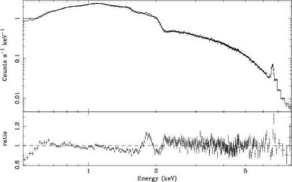
Figure 1: Fit of mekal model between 1 and 7 keV to a spectrum from the outer region of the ACIS-S3 CCD. The data were rebinned for display to have a minimum significance of $20\sigma$ per point, rebinning up to 20 channels.

At energies less than 0.6 keV the model overestimates the flux from the object. At 0.4 keV the model predicts twice as much flux as is observed. Extra absorption (at least assuming solar abundance for the absorber) does not improve the fit. We experimented using a different correction for the low energy degradation, contamarf. The results were very similar to using acisabs, except the column density increased everywhere by about $2\times 10^{20}\hbox{$\rm\thinspace cm^{-2}\,$}$.

In addition to the problems at low energy, there is a large residual around 2 keV, where the effective area of the mirror abruptly changes. This residual can be removed by adding a Gaussian near the edge. mekal or apec models cannot fit this residual if individual abundances are allowed to vary. There may also be another calibration problem starting near 1 keV, and increasing to 2 keV. It is unclear how large this effect is, as changing Ni and Mg abundances can allow the models to fit the data up to 1.8 keV, depending on the quality of the data. The residual can be fitted with a wide Gaussian, but the width of the Gaussian depends on the model fitted.

To investigate whether the residuals are new problems, or whether they exist in older data, we extracted spectra from the same region from this dataset and those used by Fabian et al (2000) and Schmidt et al (2002). The region used was a $\sim 200$ arcsec box to the South of the nucleus. There are three Chandra datasets: the one published in Fabian et al (2000) and Schmidt et al (2002) [OBS-ID 503], another just published in Schmidt et al (2002) [OBS-ID 1513], and the merged dataset we present here. In Fig. 2 we show the ratios of the data to a best fit mekal model (fitted to each dataset between 0.7 and 6 keV). The datasets were reprocessed with the latest gain files, major background flares were removed from the 503 dataset, and blank sky background spectra were used (processing these in the same way as the original dataset). Ancillary responses were corrected with corrarf.

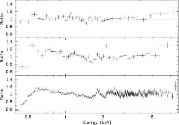
Figure 2: Ratios of models to data from identical regions for three different Chandra datasets. Top dataset was taken on 1999-11-28 (published in Fabian et al 2000, Schmidt et al 2002). Middle dataset was taken on 2001-01-29 (published in Schmidt et al 2002). Bottom dataset is our new merged dataset. The points were rebinned for display to have a minimum significance of $20\sigma$ per point, rebinning up to 20 channels.

The plot shows that the ratios to the model we see from this dataset are consistent with those from the 1513 dataset, especially around 2 keV and below 0.6 keV. The 1513 dataset shows a hard energy excess, probably as we did not make a careful enough removal of background flares for this discussion. The ratios are compatible with the 503 dataset except in the lowest energy bin.

Our main analysis technique is to split the data up into a number of independent spatial regions for separate spectral analysis (following Sanders & Fabian 2002; Schmidt et al 2002). Depending on the average quality of each spectrum, and the model we fit, we vary the procedure as described below.

If the number of counts in each spectrum is small (less than $\sim 9\times 10^{4}$) then we fit the whole energy range 0.6 to 8 keV. The data below 0.6 keV are unusable due to the drop-off in flux. The residuals around 1.8 keV are no worse than in previous observations of this object, and probably in observations of other objects with Chandra.

If the spectra we are fitting contain many counts ($\gtrsim 9\times 10^{4}$), then we exclude the region from 1.3 to 2.3 keV. This energy range was excluded from bins with $S/N\gtrsim 300$. It is a rather severe treatment of the data, but a correction of the response in this region requires knowledge of which residuals are real and which are systematic. Excluding this band means the majority of the spectra when fitted produce a reduced-$\chi^{2}$ less than 1.2, even for large spatial regions. It is important to now that much of this paper concerns the spatial distribution of temperatures, abundances etc. Provided that the systematic uncertainties have little spatial variation, the features and trends in our resulting maps will be real, although there may be small effects in the absolute values.

4 X-ray image

We show in Fig. 3 (top) a full-band image of the cluster (detailed images of the central region of the image can be seen in Fabian et al 2003a). The data were extracted using 0.25 arcsec bin (0.5 pixel bins), corrected with an exposure map, and rebinned using the bin-accretion algorithm of Cappellari & Copin (2003) with a signal to noise ratio ($S/N$) of $\sim 17$ in each bin (about 290 counts). The image was then smoothed using the natgrid natural-neighbour interpolation library. To highlight the azimuthal variation of the surface brightness, we show a ‘deprojected image’ of the same region in Fig. 3 (bottom), created by subtracting from each pixel the projected contribution from shells outside that pixel.

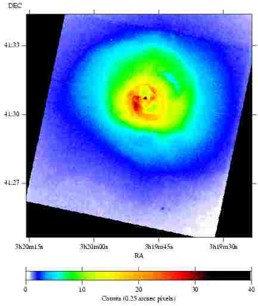
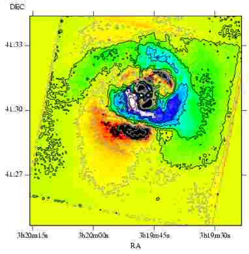
Figure 3: (Top) Full-band image of the cluster. Image was binned to have $S/N\sim 17$ in each bin, then smoothed with the natgrid natural-neighbour interpolation library. (Bottom) ‘Deprojected image’ of the core of the cluster. Areas with excess counts are shown in white (with 7 black contours, spaced with square-root scaling between 1.2 and 35 excess counts per 0.49 arcsec pixel), and areas with a deficit of counts are black (with 5 white contours, spaced linearly between -10 and -0.5 counts per pixel). The image was smoothed with a 4-pixel width Gaussian.

5 Projected temperature structure

Fig. 4 shows a detailed image of the emission-weighted projected temperature structure of the cluster (see also Fig. 6 in Fabian et al 2003a for a smoothed version).

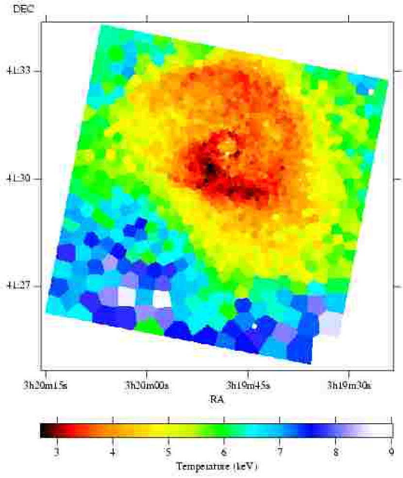
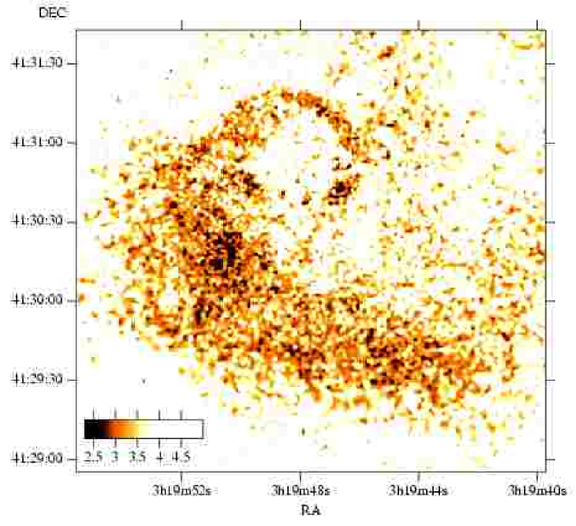
Figure 4: (Top) Projected emission-weighted temperature map of the core of the cluster, generated from fitting spectra from the $S/N\sim 100$ map. The uncertainties increase from 3-4 per cent in the centre, to 8-9 per cent in the hottest regions. (Bottom) Detail from the central region of the cluster, created from the $S/N\sim 19$ map, and smoothed with a Gaussian of 0.49 arcsec.

The data were binned spatially into 1422 regions using the bin-accretion algorithm of Cappellari & Copin (2003), with $S/N\sim 100$ ($\sim 10,000$ counts between 0.5 and 7.5 keV). The generated spectra were fit with a single-temperature mekal model absorbed by a phabs model (Balucinska-Church & McCammon 1992), between 0.6 and 8 keV, with variable absorption, abundance and temperature in each bin, fixing the redshift to the appropriate value. The results are shown plotted in Fig. 4 (top). Obvious point sources were excluded (See Table 1), shown as white circles in the temperature map (these sources have been cut out from all the maps showing the results of spectral fitting in this paper).

RA (J2000)	Dec (J2000)	Radius (arcmin)
03:19:26.79	+41:32:25.7	0.082
03:19:33.76	+41:29:56.2	0.0246
03:19:37.31	+41:29:59.1	0.0246
03:19:43.97	+41:33:04.6	0.0328
03:19:44.10	+41:25:53.7	0.0738
03:19:48.09	+41:31:01.7	0.0246
03:19:48.17	+41:30:42.5	0.041
03:19:56.11	+41:33:15.5	0.0328
03:20:01.45	+41:31:27.2	0.0328

Table 1: Excluded point sources, sorted by RA.

We created a version of the map with higher spatial resolution, the central region shown in Fig. 4 (bottom). The temperatures in this map have large uncertainties, but it shows the morphology well. To create the high resolution map, the data were again spatially binned with $S/N\sim 19$ ($\sim 360$ counts per spectrum between 0.5 and 7.5 keV), producing 37,811 spatial regions, from which spectra were extracted. Each spectrum was fit with the same model, but using a fixed abundance and absorption with the appropriate values obtained from the $S/N\sim 100$ map, only allowing the temperature and normalisation to vary (This is similar to the procedure used by Schmidt et al 2002). The spectra were fit using $C$ statistics (Cash 1979) rather than $\chi^{2}$ statistics, a fit statistic more appropriate in the low signal-to-noise regime. We fit the spectra between 0.6 and 5 keV. Instead of calculating individual responses and backgrounds for each spectrum, we used the appropriate ones corresponding to the nearest $S/N\sim 100$ bin.

There is a considerable level of apparent structure in the temperature distribution. For instance there are number of cooler clumps in the region of bright emission to the south-east and south of the innermost southern radio lobe. If we fit the spectrum of the largest cool clump at (03:19:50.8, +41:30:13) then we obtain a temperature of $2.4\pm 0.2$ keV. There are also some hot features in the outer part of the cluster, for example there is a $\sim 20$ arcsec radius region near (03:20:03.4, +41:26:59) consisting of a clump of hot bins. The best fitting temperature of that region is $9.0\pm 0.55$ keV. An additional clump near (03:19:37.9, +41:25:37) has a best fitting temperature of $10.3^{+1.5}_{-1.4}$ keV. Comparing the temperature structure against the locations of galaxies, there appear to be a number of galaxies which appear to lie along the low temperature swirl around the core. Many of the smallest scale (few arcsec) structures seen in the detailed temperature map (Fig. 4 [bottom]) are likely to be noise, but coherent structures seen in the X-ray surface brightness maps from the brightest part of the cluster suggests there are likely to be temperature variations on this scale. Examination of maps with intermediate resolution reveals structures cooler than their surroundings by $\sim 0.6$ keV on scales of $\sim 2.5$ arcsec (1 kpc).

In Fig. 5 we show the radial and angular plots of the temperatures obtained from the larger scale $S/N\sim 100$ fits. The plot highlights the cool rims around the regions associated with the radio lobes, the fairly flat, cool region of emission to the south of the core, and the temperature increasing in the outer parts. Also the wave-like ripples in the temperature structure caused by the cool swirl are visible as a function of angle.

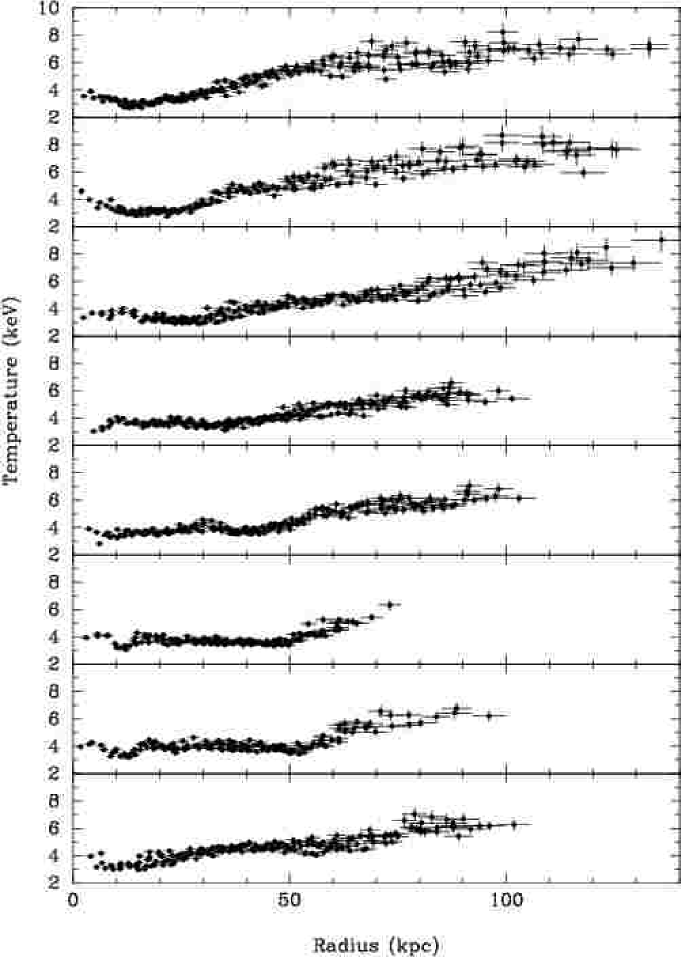
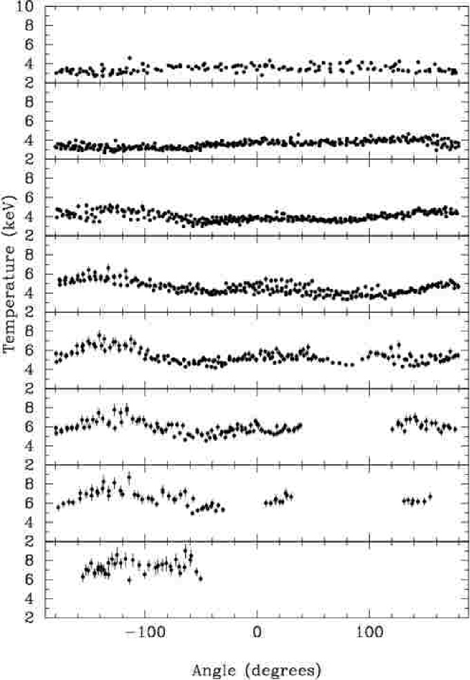
Figure 5: Left: temperature of each spatial bin in the $S/N\sim 100$ temperature map as a function of radius (kpc), divided up into eight annular sectors at multiples of $45^{\circ}$. The panels progress in a anti-clockwise direction, with the first panel spanning between East and South-East. The horizontal error bars indicated the RMS radius of the pixels in each bin, the vertical error bars indicate the $1\sigma$ uncertainty on the temperature. Right: temperature of each spatial bin as a function of angle (measured anti-clockwise with $0^{\circ}$ as the West), divided into eight radial annuli. The top panel shows the first annulus (inner 15 kpc), moving out by 15 kpc for each subsequent panel. The final panel also shows all remaining points.

5.1 Absorption structure

Looking for the signature of absorption in the dataset is a difficult process. The first problem is the calibration problems below 0.6 keV, the second the variation of the degradation of the low energy response with position. It is thought this degradation is caused by build-up of material on the filter in front of the detector (Marshall et al 2003), and is more prevalent in those regions where the filter is cooler. We show the variation of the best-fitting hydrogen absorption (assuming solar absorber) as a function of position in Fig. 6, binning spectra spatially with $S/N\sim 100$. This map does not include any correction for the spatial dependence of the QE degradation, but does include corrarf correction for the average effect. This map was produced by the same set of spectral fits as the temperature map plotted in Fig. 4 (top), and smoothed with natgrid.

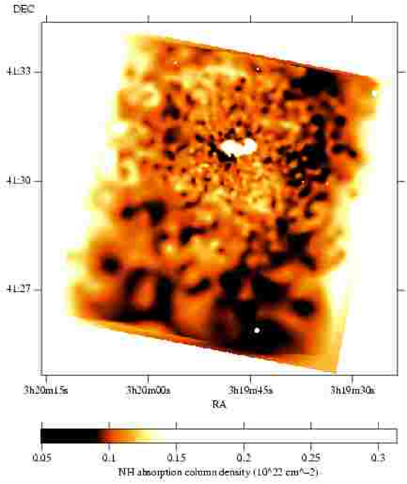
Figure 6: Map of $N_{H}$ (galactic plus intrinsic plus instrumentational), derived using bins with $S/N\sim 100$. The data were smoothed with natgrid.

The Galactic column density towards the Perseus cluster is uncertain as it lies at low galactic latitude. The value obtained from Dickey & Lockman (1990) is $N_{H}\sim 1.5\times 10^{21}\hbox{$\rm\thinspace cm^{-2}\,$}$. Most of the values we measure are below that. The values in our absorption map are $\sim 2\times 10^{20}\hbox{$\rm\thinspace cm^{-2}\,$}$ greater systematically if we use the contamarf correction rather than corrarf.

The east-west absorption feature near the centre of the cluster is associated with the high-velocity system (HVS), which we discuss separately in Gillmon et al (2003). Along the east and west edges of the CCD are regions of high absorption, which may be where there is build-up of material on the detector. The level of absorption appears to decrease from the E-W edges to minima about $1/4$ and $3/4$ of the distance along the edge, but then there is an increase of absorption again towards the centre. There are enhancements especially to the edges of the cool swirling region at the centre, in particular near (03:19:53.8 +41:32:50) and (03:19:43.7 +41:29:26). In addition there is an enhancement below the position of the southern outermost radio lobe. It appears that where gas is cooler we see more absorption.

It is very difficult to say for certain that the features we see are real. The absorption map produced seems fairly independent of spectral model and the signal to noise of the spatial binning; variable abundance and variable abundance cooling flow models produce similar maps. The effect may however be an artifact of the QE degradation or another calibration problem, but it is interesting to note that the features in the absorption map correspond to features in the cluster, although this would be the case if the spectral model is incorrect. We stress that the QE degradation is position dependent.

5.2 Velocity structure

Dupke & Bregman (2001) pioneered the use of ASCA GIS spectra to measure velocities in the Perseus cluster. The region of the cluster we can probe with this observation is much smaller, so we cannot compare our results with theirs.

Our initial attempts to measure the velocity structure were thwarted by a systematic caused by the response matrix energy binning. The redshift distribution was discretised into values separated by the response matrix energy bin size. To avoid this problem we used a width of 0.5 eV in the response matrices used in this section, rather than the usual value of 10 eV. In addition early versions of the correction of the time dependence of the gain did not completely correct the problem, due to a bug in mkrmf. In this section we use the November 2003 release of corr_tgain rather than the Summer 2003 release.

We extracted spectra from bins with $S/N\sim 500$ (about $2.5\times 10^{5}$ counts). The spectra were fitted using a mekal model between 3 and 8 keV, with the temperature, abundance, normalisation and redshift free parameters. We used $C$ statistics on unbinned spectra. This spectral region was used as the Fe-K lines are the best indicators of velocity structure, as the centroid of the Fe-L complex is more difficult to determine and its spectral region is contaminated by emission from other elements.

The mean redshift found was $0.0169\pm 0.0001$ (Fig. 7 [top]), with a standard deviation, $\sigma_{z}$, of $7.7\times 10^{-4}$, which is close to the mean error on each redshift, $6.6\times 10^{-4}$. $\sigma_{z}$ corresponds to a velocity of $230\hbox{$\rm\thinspace km\rm\thinspace s^{-1}\,$}$. The distribution of velocities is compatible with there being a single component. The smallest scale we are sensitive to is $\sim 30$ arcsec (12 kpc). However, with higher signal to noise ($S/N\sim 700$, about $4.9\times 10^{5}$ counts), we appear to find significant structure in the redshift map (Fig. 8). The bins marked $A$ and $B$ are moving towards us with respect to regions $C$ and $D$. The relative velocity of the two pairs is $\sim 570\hbox{$\rm\thinspace km\rm\thinspace s^{-1}\,$}$. The linear structure is reminiscent of a galactic rotation curve, but could also be due to the radio jets from the centre (although there is no simple agreement with the configuration of the jets).

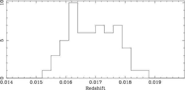
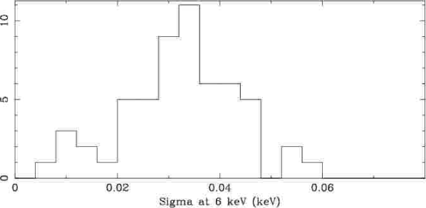
Figure 7: (Top) Distribution of the best-fitting redshifts in each bin. The mean 1$\sigma$ error on each value is $6.6\times 10^{-4}$. (Bottom) Distribution of the gsmooth smoothing $\sigma$, measured at 6 keV. The mean error on each value is $\sim 0.01\rm\thinspace keV$.

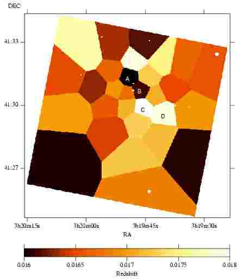
Figure 8: Redshift distribution generated from a $S/N\sim 700$ map. Typical errors are $\sim 0.0005$. The bins marked $A$, $B$, $C$ and $D$ have redshifts of $0.0160\pm 0.0004$, $0.0161\pm 0.0003$, $0.0180\pm 0.0005$ and $0.0179\pm 0.0003$, respectively.

In addition to this simple analysis, we fitted the same mekal model convolved with a Gaussian (the gsmooth model in xspec with an energy power index of 1), to test for a velocity spread on the Fe-K lines. Neither the apec nor mekal models include thermal broadening effects on the emission lines. If there is no turbulence, a 4 keV plasma will show a broadening of $\sim 2.6$ eV for the Fe-K lines. Unexpectedly, we found a significant extra line width in the spectra from most bins (Fig. 7 [bottom]), with a mean of $32.2\pm 0.1$ eV at 6 keV, corresponding to $1600\hbox{$\rm\thinspace km\rm\thinspace s^{-1}\,$}$. The $1\sigma$ error on each value was $\sim 10$ eV. To demonstrate the strength of the signal we show a spectrum in Fig. 9 from one of the bins fitted with a model without smoothing. The residuals in the wings of the line are easily visible. We also checked that apec models gave similar deviations. We note that this result may be instrumental, for example due to charge transfer inefficiency of the detector.

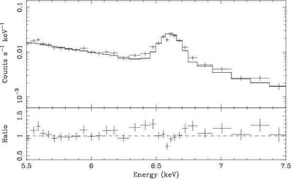
Figure 9: Detail around the Fe-K lines to demonstrate that a mekal model is too narrow to fit the data without smoothing. The data have been rebinned to have a signal-to-noise of 10 in each bin, grouping together a maximum of 30 channels.

We note that the mean redshift found is not the nominal redshift of the cluster. The offset corresponds to a velocity of $420\hbox{$\rm\thinspace km\rm\thinspace s^{-1}\,$}$. It is possible that this may be caused by a systematic gain shift, although we have corrected the gain in the data using corr_tgain.

6 Abundance structure

6.1 Fixing abundances at solar ratios

Fig. 10 shows an emission-weighted abundance map produced by fitting a single temperature model (the same model as in Section 5) to spectra extracted from a $S/N\sim 150$ binned map. We did not allow redshifts to vary here, but we do in Section 6.2. The abundances were measured assuming solar abundance ratios, although the elemental abundance we are most sensitive to is Fe. The abundance map shows a substantial amount of structure. The overall pattern is that the abundance appears to rise to a peak around 100 arcsec (37 kpc) to the NW and 60 arcsec to the SE. There is an abundance enhancement in the outer SW part of the map. Inside this radius the abundance drops down, especially to the W side of the cluster.

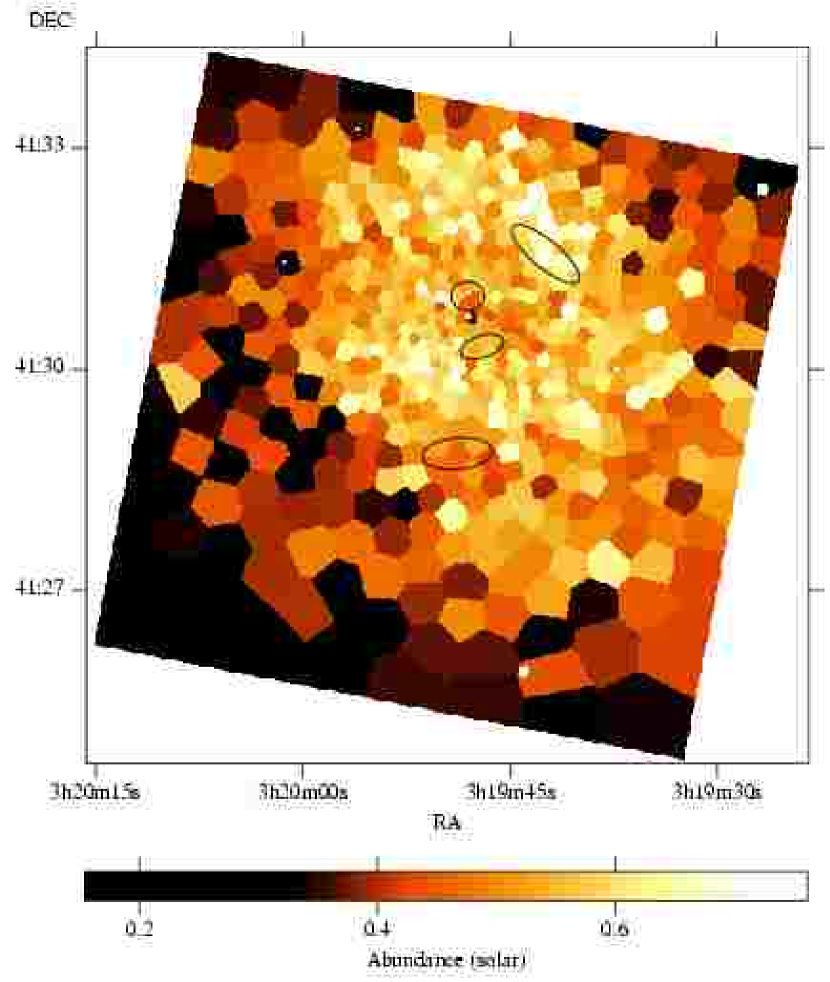
Figure 10: Map of abundance using bins with $S/N\sim 150$. The uncertainties on the abundances rise from about $0.04$ in the centre to about $0.08\hbox{$\thinspace\mathrm{Z}_{\odot}$}$ in the outer regions. The ellipses mark the approximate positions of the radio lobes.

The morphology of the abundance map follows the temperature map (Fig. 4) closely. Those regions with low temperatures generally have high abundances. We can quantify this somewhat by plotting the abundance of bins against their temperature, which is shown in Fig. 11. The uncertainties on the temperatures and abundances for a particular bin are correlated, but the correlation is that uncertainties in abundance increase with increasing uncertainties in temperature, which is the opposite sense to the trend in the best-fitting values. By faking a dataset with the same emission-weighted temperature distribution as the real cluster (measured from a $S/N\sim 225$ map), but with a constant abundance of $0.5\hbox{$\thinspace\mathrm{Z}_{\odot}$}$ everywhere, and repeating the analysis, we verified there was no significant systematic effect we could find to account for this trend. There is a minor systematic effect in the procedure, with a decrease of $0.05\hbox{$\thinspace\mathrm{Z}_{\odot}$}$ over the temperature range observed.

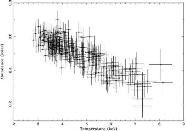
Figure 11: Plot of abundance against temperature for each bin, generated from a $S/N\sim 225$ map. The same relation exists for the $S/N\sim 150$ map, but with larger uncertainties.

There are a number of high-abundance ‘clumps’, for example at (03:19:40.9 +41:31.21) where $Z=0.68\pm 0.05\hbox{$\thinspace\mathrm{Z}_{\odot}$}$, (03:19:49.3 +41:29:59) where $Z=0.67\pm 0.04\hbox{$\thinspace\mathrm{Z}_{\odot}$}$. and (03:19:34.6 +41:29:51) where $Z=0.70\pm 0.05\hbox{$\thinspace\mathrm{Z}_{\odot}$}$ (its surrounds are at $0.47\pm 0.02\hbox{$\thinspace\mathrm{Z}_{\odot}$}$). Many of these regions have scales of around 20 arcsec. The existence of small-scale inhomogeneities in the abundance distribution was hinted at by Schmidt et al (2002). There is also a low abundance linear ($Z\sim 0.5\hbox{$\thinspace\mathrm{Z}_{\odot}$}$) feature from the core to at least 60 arcsec WSW (this is more easily visible using high $S/N$ binning: see Fig. 14).

One high abundance peak is associated with the position of the outer NW radio lobe. The material just within the radius of the lobe has a mean abundance of $\sim 0.53\pm 0.01\hbox{$\thinspace\mathrm{Z}_{\odot}$}$, whilst the material at the radius of the lobe or just beyond has an abundance of $0.62\pm 0.015\hbox{$\thinspace\mathrm{Z}_{\odot}$}$. There may also be an enhancement in abundance corresponding with the position of the inner SW radio lobe. The gas along the line of sight of the inner NE lobe does not have an obvious enhancement, but the material further away in radius is enhanced. There is some enhanced abundance gas lying outside the outer S radio lobe.

In Fig. 12 we plot the abundance as a function of radius and angle. The plots, in particular the abundance as a function of angle, highlights that the metals are not uniformly distributed. The abundance dips and peaks by magnitudes of up to $0.1-0.2\hbox{$\thinspace\mathrm{Z}_{\odot}$}$.

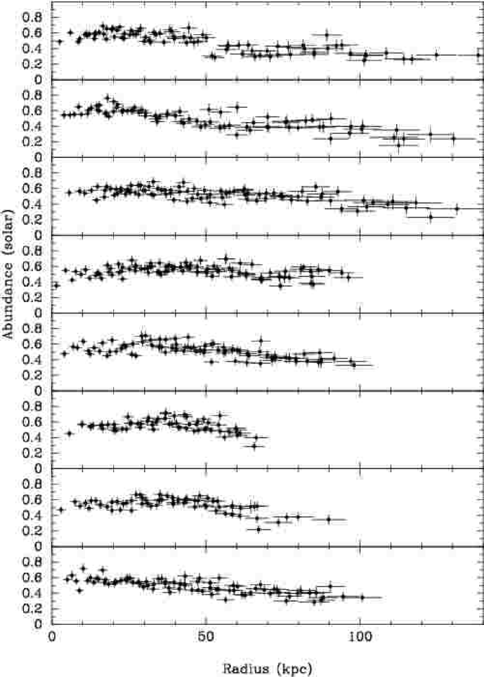
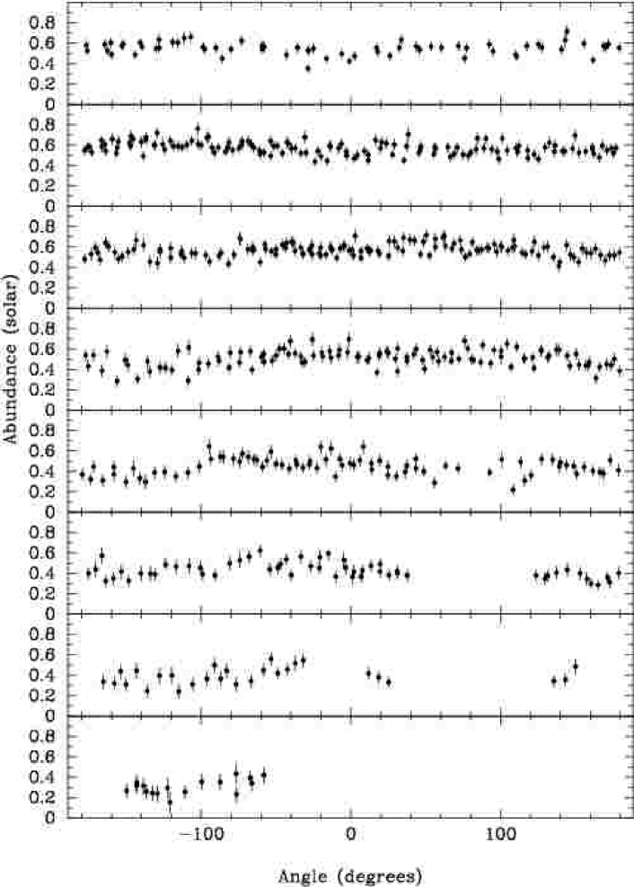
Figure 12: Radial and annular abundance profiles for each bin in an abundance map generated from a $S/N\sim 150$ binned image. See Fig. 5 for an explanation of the coordinate system.

The abundances we measure may be subject to further systematic errors. The gas in the cluster may be optically thick to resonantly scattered lines (e.g. Gilfanov, Sunyaev & Churazov 1987), however Dupke & Arnaud (2001), Churazov et al (2003b), Gastaldello & Molendi (2003) observe no evidence for resonant scattering in this cluster. Another effect is known as ‘Fe-bias’ (Buote 2000), where one underestimates the abundance of the emitting gas if it consists of more than one phase. However we test for the presence of multiple components in Section 7, and allow for projection effects in Section 8.

6.2 Allowing individual abundances to vary

By fitting a vmekal or vapec model to the spectra extracted from each bin we can make maps of individual elemental abundances. To demonstrate the excellent signal-to-noise of the data, we show in Fig. 13 the contributions to a spectrum by the various metals (We note that residuals are also seen in Fig. 13 where emission lines due to Ti and Cr are expected, but only Cr has a plausible strength). By excluding the energy range 1.3–2.3 and below 0.6 keV (where we are most uncertain about the calibration) the fits are not sensitive to Mg or Si abundances. The elements we fit for are Fe, Ar, Ca, Ne, O, Ni and S. Other abundances remain frozen at solar values. Excluding effects such as resonant scattering and Fe-bias, the Fe abundance is the most secure. O abundances could be problematic as O emission lines lie close to 0.6 keV, and could be affected by systematics errors near that limit. Ni and S abundances have larger uncertainties than could be obtained from the full energy range, as some of their lines are in the 1.3-2.3 keV region.

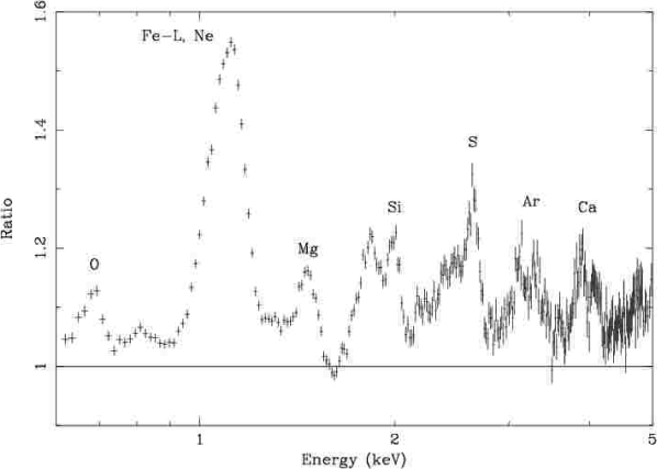
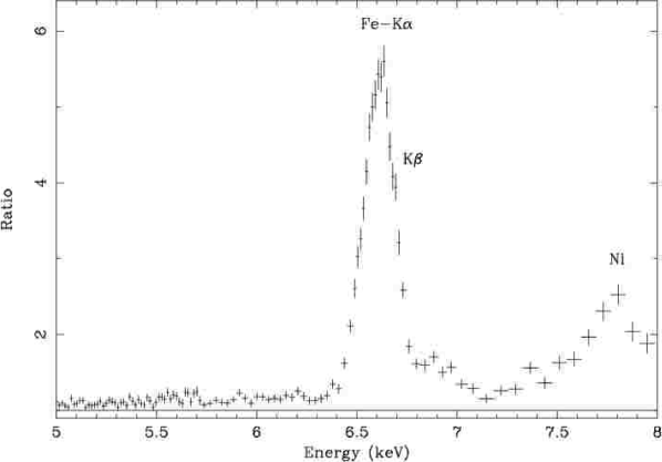
Figure 13: Ratio of a best fitting vmekal model (after setting the O, Ne, Mg, Si, S, Ar, Ca, Fe and Ni abundances to zero) to a spectrum extracted from an annulus from radius 130 to 200 arcsec (26 kpc wide). Visible are O, Fe-L, Mg, Si, S, Ar, Ca, Fe-K and Ni lines. Both the hydrogenic and helium-like lines of S, Ar and Ca are seen.

We plot the Fe, Ni, and Ne abundances obtained from a vmekal fit to data extracted from a $S/N\sim 300$ map in Fig. 14 (top row). We also created maps of O, Ca, Ar and S abundances, which we do not show here. When fitting the data the temperature, absorption, abundances and redshift of the gas were allowed to be free. The redshift was allowed to vary as the best fitting redshift is not the nominal redshift of the cluster. We also tested the approach fitting the data with fixed redshift, and using $C$ statistics instead, yielding very similar results to those presented here.

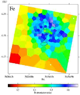
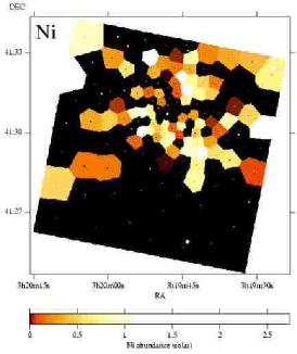
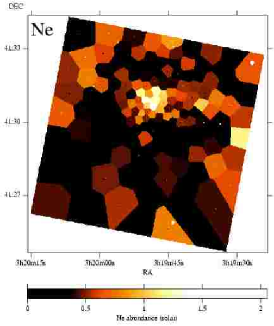
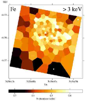
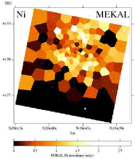
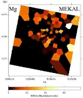
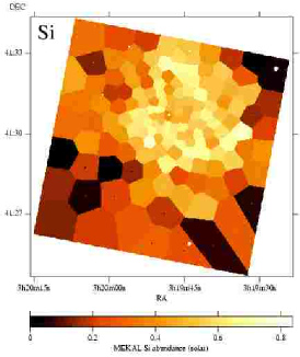
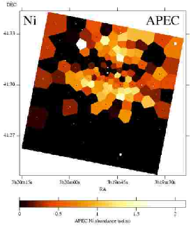
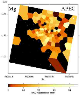
Figure 14: Maps generated by fitting spectra with $S/N\sim 300$. (Top Row) Fe, Ni and Ne maps, generated by fitting a vmekal model excluding the energy range 1.3-2.3 keV. (Centre Left) Fe-K map, generated by fitting spectra above 3 keV. (Centre Centre, Centre Right, Bottom Left) Ni, Mg and Si maps created by fitting vmekal models to 0.6-8 keV. (Bottom Centre, Bottom Right) Ni and Mg maps from fitting vapec models to 0.6-8 keV. The boxes within each bin mark the $1\sigma$ uncertainties.

The Fe abundance map shows a very similar pattern to the overall abundance map (Fig. 10), highlighting the apparently low abundance extension to the W, the abundance peak near the outer NW radio lobe and to the SE, and the drop in abundance to the centre.

The Ni map indicates there is very little evidence of Ni enrichment in the S of the cluster; the black areas on the map are all upper-limits. Around the core of the cluster there is a ring-like feature of high abundance. Near the core the Ni abundance is apparently zero again.

The Ne abundance shows a simpler pattern. The abundance rises towards the centre. Most of the bins at the centre have supersolar Ne abundances. There are a number of features, though, that appear significant. There is a low abundance feature to the SE of the core (centred near 03:19:58.4, +41:30:09), and another to the bottom SE of the map.

The other abundance maps have less-clear patterns to them. The Ca abundance appears to be quite patchy. Binning up the data further identifies an arc of high abundance and low statistical significance to the W and S of the cluster, about 90 arcsec from the nucleus. The Ar abundance map is similarly patchy, with a high abundance to the NW. The O abundance map has a rather strange morphology. There are a number of low and high abundance regions, some apparently linear in shape. The O abundance appears low near the core. The odd O abundance pattern suggests it is the result of a systematic error, particularly as its emission lines lie at low energy.

We overplotted the abundance maps with positions of cluster members. Curiously the locations where Ni is enhanced appears to coincide with the positions of galaxies in the cluster. It is difficult, however, to justify this physically as the galaxies (except for NGC 1275) are probably moving rapidly and so there should be little significant enrichment to their current surroundings. A galaxy is likely to only remain in one of the bins for $\sim 10^{7}$ yr.

We fitted the abundances at the position of the outer NW radio lobe and within that region, yielding the values in Table 2. It appears the projected abundances of O, Ar, Ca, Fe and Ni are smaller within the lobe, whilst Ne is larger (as expected from the maps above). There is no trend in S abundance.

Element	O	Ne	S	Ar	Ca	Fe	Ni
Within	$0.37\pm 0.06$	$0.70\pm 0.07$	$0.61\pm 0.05$	$0.35\pm 0.12$	$0.25\pm 0.12$	$0.54\pm 0.01$	$<0.14$ (1$\sigma$)
Without	$0.53\pm 0.08$	$0.31\pm 0.08$	$0.60\pm 0.06$	$0.95\pm 0.15$	$0.81\pm 0.16$	$0.62\pm 0.015$	$0.54\pm 0.28$

Table 2: Abundances just within the position of the outer NW radio lobe, and at the position of the lobe and just beyond.

In addition to the fits to the energy range 0.6-1.3, 2.3-8 keV, we fit the data in other energy bands. In Fig. 14 (centre left) we show an Fe-K map, created by fitting the data above 3 keV with Fe, Ar, Ca and Ni free. The map is similar to the one based on Fe-L and Fe-K lines but there are some differences. The abundances are higher by about $0.05\hbox{$\thinspace\mathrm{Z}_{\odot}$}$ in the outer regions to the S, lower towards the centre (by about $0.04\hbox{$\thinspace\mathrm{Z}_{\odot}$}$), except to the W of the nucleus where the abundances are higher (by $\sim 0.03\hbox{$\thinspace\mathrm{Z}_{\odot}$}$). To the W of the nucleus the low-abundance feature is not as prominent.

We also computed maps for Mg, Si and Ni, using the full band between 0.6 and 8 keV and ignoring the systematic effects. Since we do not understand the nature of these residuals the maps must be treated with caution. We show the vmekal Si map in Fig. 14 (bottom left). The vapec map is similar. The Si abundance follows the Fe abundance closely, rising to a peak away from the nucleus and dropping down at the centre. We show separate vmekal and vapec maps for Mg and Ni as there are substantial differences between the models. vapec has stronger Mg than vmekal, but weaker Ni.

7 Multiple temperature component analysis

As we mentioned in Section 6.1, if we use the incorrect number of temperature components in our fits it may lead to an underestimate of the abundance. It may be the case that in the centre of the cluster, where there is most likely to be multiphase gas, the abundance is being underestimated. In particular the solar, Fe and Ni abundance drops seen in Fig. 10 and Fig. 14 may be systematic effects. We therefore have attempted to fit multiple temperature components to the extracted spectra.

If there are multiple phases, and assuming they are in pressure equilibrium, an expression giving the volume-filling-fraction (VFF; see equation 1 of Sanders & Fabian 2002 for the two-phase version) of the $i$th phase ($f_{i}$) is given by

$$f_{i}=\frac{K_{i}\>T_{i}^{2}}{\sum_{j}K_{j}\>T_{j}^{2}},$$ (1)

where $K_{i}$ is the normalisation of the $i$th phase (proportional to its emission measure), and $T_{i}$ is its temperature.

We fitted a model made up of a number of fixed temperature components with variable normalisations, tying their abundances together. The temperature components started with one at 0.5 keV, increasing in temperature by factors of two until 16 keV. This approach has the advantage that we can test for the presence of gas close to a particular temperature. In addition the temperatures of a component do not jump to very high or low values in the fit depending on initial fit parameters; in our model the normalisation of a component simply drops to zero if there is no gas near that particular temperature. If the gas is single-phase but not at the temperature of one of our components, then we will detect it at the temperature of the neighbouring components.

We also fit a model consisting of a temperature component, its temperature free in the fit, and components at fixed fractions of that temperature ($1/2$, $1/4$ and $1/8$). The results from this alternative model appear to be consistent with those from this model.

In Fig. 15 is shown the VFF of each temperature component in each bin. The 0.5 keV map shows a diffuse very low VFF component covering the image. There is some enhancement towards the centre of the cluster. It is possible this is a real effect, but this map is sensitive to the calibration at low energies and could be plagued by systematic errors. At 1 keV, there are only upper limits in most bins, except in the very core and in a band running in a NE-SW direction in the SE of the image. At 2 keV there is a great deal of gas. Most of this gas follows the morphology as the cool gas in the single-phase temperature map (Fig. 4). Looking at the 4 keV map, most of that gas with a high VFF occupies the region of the low-temperature swirl, but there is a large clump to the SW of the nucleus. In addition there is a diffuse halo of hotter gas outside of the inner core, corresponding to what we would expect from the mean temperature of the gas there. When we reach 8 keV, we only see gas in the outer parts of the cluster, except for a W-E band to the N of the nucleus, corresponding in position with the high-velocity system. The 16 keV map is rather unusual in that it shows a region of hot emission around the core, but not so much in the outer regions where the mean temperature is hottest, or to the S of the nucleus where it is coolest.

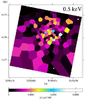
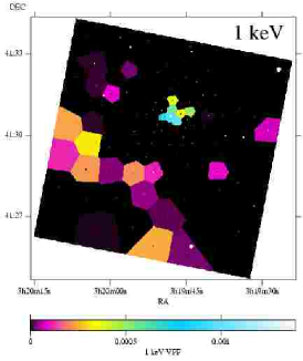
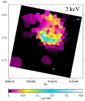
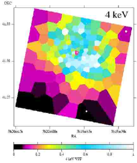
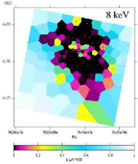
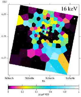
Figure 15: Volume-filling-fractions of components starting at 0.5 keV, and increasing in temperature by factors of two. The maps were generated by fitting spectra extracted from a $S/N\sim 300$ map with a vmekal model with multiple temperature components. The boxes within each bin mark the $1\sigma$ uncertainties on the VFF, assuming there is only uncertainty on the normalisation of that component.

We also repeated the analysis on a faked dataset. The faked dataset was generated from real $S/N\sim 225$ projected temperature, abundance, normalisation and absorption maps, faking a spectrum using xspec for each detector pixel, and populating an events file with the events necessary to create each detector pixel spectrum. The faked data has a single temperature component at all location, and includes no projection effects. The 0.5 keV faked map shows some points at the values observed in the real data, but the majority of bins have smaller VFFs than the real data. The 1 keV faked map shows no concentration of VFFs at the centre. The 2 and 4 keV maps are similar to their real counterparts. The 8 keV map resembles the real map, but does not have the band of high VFFs running across the N of the nucleus. The 16 keV map shows a few random points with significant VFFs, and does not show similar structures to those seen in the real data.

If we examine the Fe abundance obtained by a multiple component fit, the Fe abundance still declines in the centre, and along the low abundance SW extension from the core. We can divide the Fe abundance map with the single-component map (Fig. 14), the result of which is shown in Fig. 16. It appears that introducing multiple temperature components does not increase the abundance over much of the central region, except in the innermost few bins. If we fit the data with the temperature components separated by a ratio of 1.5 instead of 2 then we do not see a significant change the abundance map. We also do not see a difference using the alternative model that consists of a free upper fitted temperature with fractional temperatures below that.

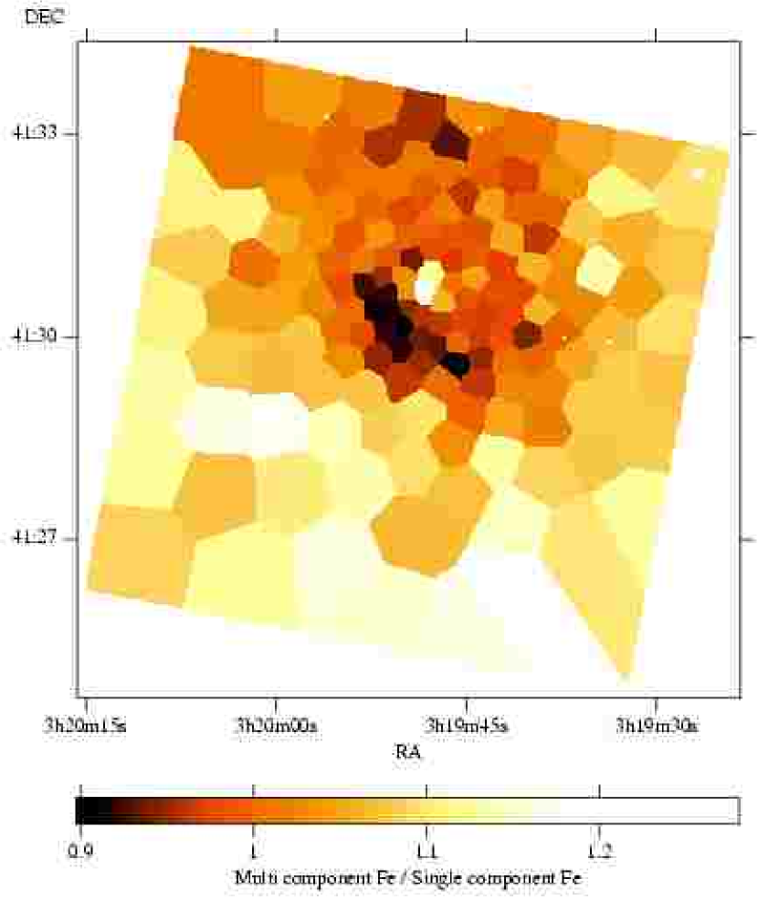
Figure 16: Ratio of the multiple component Fe abundance to the single component Fe abundance

7.1 Cooling flow model

We can fit an isobaric cooling flow model (Fabian 1994; Johnstone et al 1992) in which the gas is cooling from an upper temperature ($kT_{\mathrm{upper}}$) to a lower temperature ($kT_{\mathrm{lower}}$), at a certain rate ($\dot{M}$). The cooling flow model we use is based on the vmekal spectral model, with variable abundances. We excluded the range 1.3-2.3 keV in the spectral fitting. Fig. 17 shows $kT_{\mathrm{lower}}$, $kT_{\mathrm{upper}}$ and $\dot{M}$.

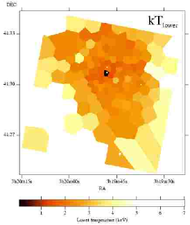
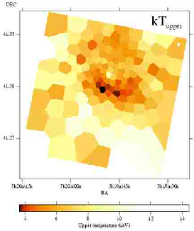
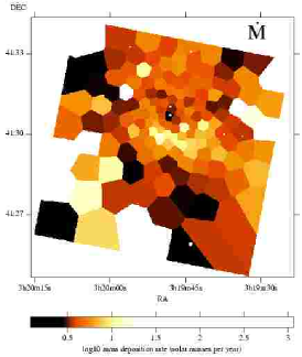
Figure 17: Results of fitting cooling flow model to the spectra extracted from the $S/N\sim 300$ bins. Left panel is the lower temperature of the cooling flow, the middle panel is the upper temperature, and the right panel is the mass deposition rate in each bin.

Those regions where $kT_{\mathrm{upper}}$ is close to $kT_{\mathrm{lower}}$ at the edges of the image should be ignored, as the mass deposition rate is meaningless. The $kT_{\mathrm{lower}}$ distribution is fairly flat over the core of the cluster, but lowest near the central source. The $kT_{\mathrm{upper}}$ distribution is lowest where the projected temperature is lowest. The most significant mass deposition rates are where the projected temperature is lowest. If we sum the total mass deposition rate where the projected temperature is lowest, we find $\dot{M}\sim 255\hbox{$\hbox{$\rm\thinspace M_{\odot}$}\rm\thinspace yr^{-1}\,$}$. However $kT_{\mathrm{lower}}$ is 2 to 2.5 keV over much of this region, in agreement with the results of on the lack of low energy gas seen in other clusters (e.g. Peterson et al 2001, 2003).

8 Accounting for projection

The above analyses do not take projection effects into account. In order to account for projection, we have to assume some symmetry. The maps in the previous sections show that the cluster is not symmetric in its core, and so it is not possible to perfectly account for projection effects. To account for the variation as a function of angle, we divided the cluster into a number of sectors.

We divided each sector into a regular set of partial-annuli, and performed spectral fitting accounting for projection effects using the xspec projct model. The spectra were fit from the outermost annulus inwards, fitting the parameters for an annulus, and freezing its parameters when fitting interior annuli. Annuli were fit without including in the fit the data from any interior annuli. We fit the absorption for each shell as Fig. 6 reveals that there is a large deal of systematic variation and possibly intrinsic variation. The value of $N_{H}$ from this projection model may not mean very much if the absorption is intrinsic to the object.

This procedure has the advantage that parts of the cluster which do not fit correctly assuming spherical symmetry or for which our spectral model does not fit the data well, do not affect the parameters of exterior annuli. It has the disadvantage that the statistical weight of interior annuli does not feed into the fitting of a spectrum. Additionally, the uncertainties we calculate using the usual $\Delta\chi^{2}$ approach do not include the uncertainties on the parameters for exterior annuli. A result of our approach may be oscillatory profiles, where a parameter is underfit on one annulus, and subsequently overfit on the next innermost annulus. Indeed the results from outermost annuli must be taken with caution as the projection model does not know what volume the gas emitting in the shell occupies, as we do not account for projection to the edge of the cluster. Our analysis will fail for regions where spherical symmetry within a sector cannot be assumed.

8.1 Simple single-temperature model

Firstly we conducted a simple mekal fit accounting for projection, to fit for the temperature, absorption and abundance. In Fig. 18 is shown the temperature of each sector, its electron density, the mean radiative cooling time, and its entropy. Sectors occupied by the radio lobes or where the projection model failed are not shown. The electron density was calculated from the emission measure of the model in each partial annulus. The mean radiative cooling time was found by taking the ratio of the thermal energy of the gas to its luminosity, and the entropy was calculated using the relation $S=kT\>n_{e}^{-2/3}$. By multiplying the temperature of each sector by its electron density we created a pressure map, shown in Fig. 19 (Left). To convert the electron pressure to total pressure, multiply by a factor of 1.9. The azimuthal symmetry seen in this map, with for example no ‘swirl’ evident, argues against significant non-hydrostatic pressure sources such as bulk motions. If we compute the ratio of the standard-deviation to the mean of the pressure in the annulus where the low temperature swirl is most prominent (sector 8 from the centre), we find a spread of 6.7 per cent. This is much less than the spread of the density (14 per cent) or of the temperature (15 per cent). As inspection of Fig. 21 reveals, local offsets in the temperature are anti-correlated with local offsets in density. The low temperature swirl does not therefore indicate recent bulk motion in the gas (although the denser gas must presumably sink). A detailed temperature map of the core is shown in Fig. 20. The radii of the sectors used were matched to the radii of the rims and other features.

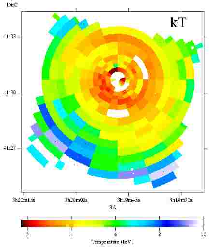
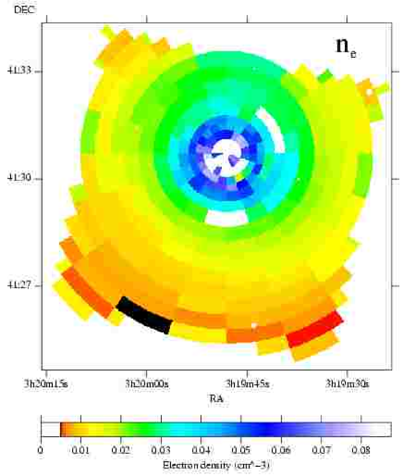
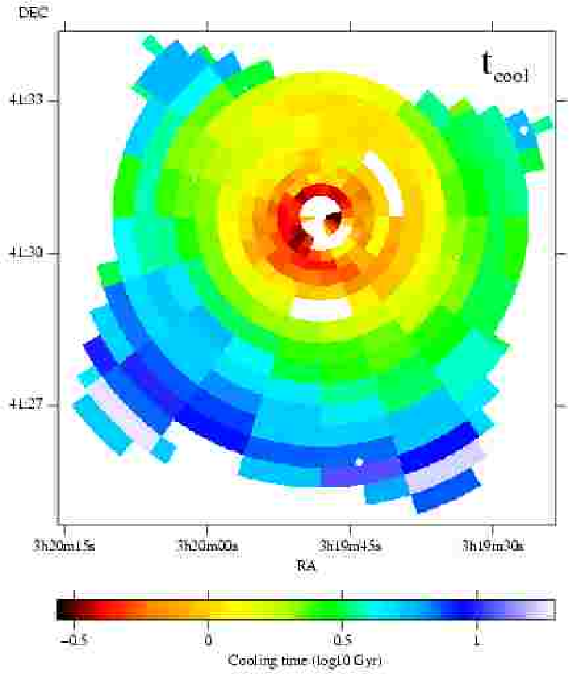
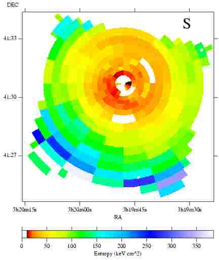
Figure 18: Temperature, density, cooling time and entropy plots, generated by fitting spectra in twenty sectors, accounting for projection effects. The boxes within each bin on the temperature plot mark the $1\sigma$ uncertainties. Sectors in which the radio lobes are located or projection effects failed are not shown. These values are plotted in Fig. 21.

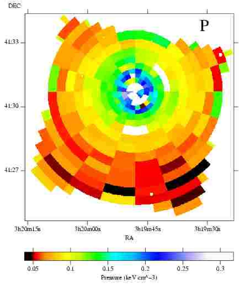
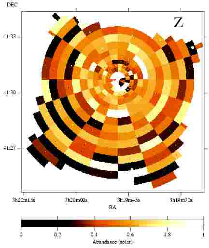
Figure 19: (Left) Pressure map of the cluster, accounting for projection. (Right) Abundances of sectors. The boxes within each sector mark the $1\sigma$ uncertainties.

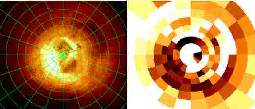
Figure 20: (Left) Regions used in the projection analysis on an intensity image of the centre of the core. (Right) A temperature map of the same sectors, from $\sim 2$ keV in black to $\sim 4$ keV or more in white (or where the spherical symmetry assumption fails).

Fig. 5 shows that we do not see temperatures below 3 keV in the projected temperature analysis. Accounting for projection, we see some temperatures below 2 keV on the N edge of the radio lobe. In the innermost 40 arcsec of the cluster the analysis accounting for projection effects fails and the temperatures become unconstrained. This is because there is too little emission than expected from projection alone. Therefore there is more emission from gas on the plane of the sky than along the line-of-sight, and the structures we observe are not spherically symmetric.

Accounting for projection by assuming spherical symmetry also appears to fail in the outer NW radio lobe, which we discuss separately in Section 9. However, for much of the cluster the morphology of temperature follows the morphology of the projected temperature map closely (Fig. 4).

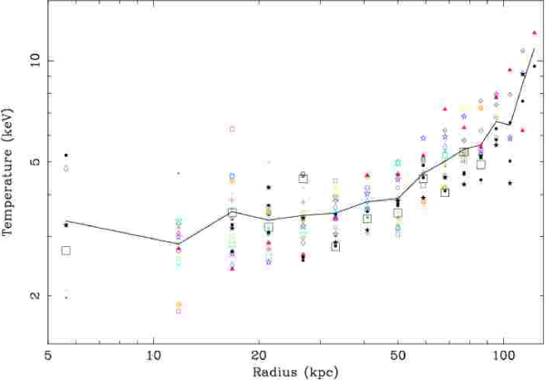
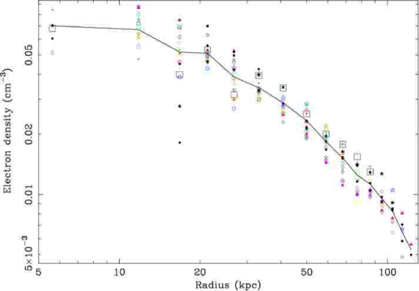
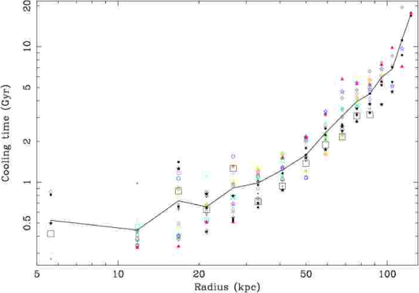
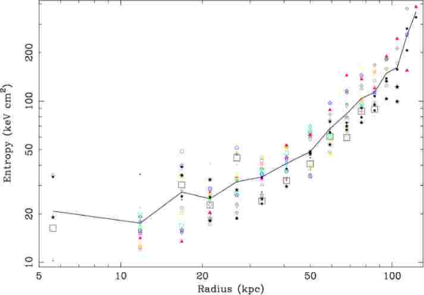
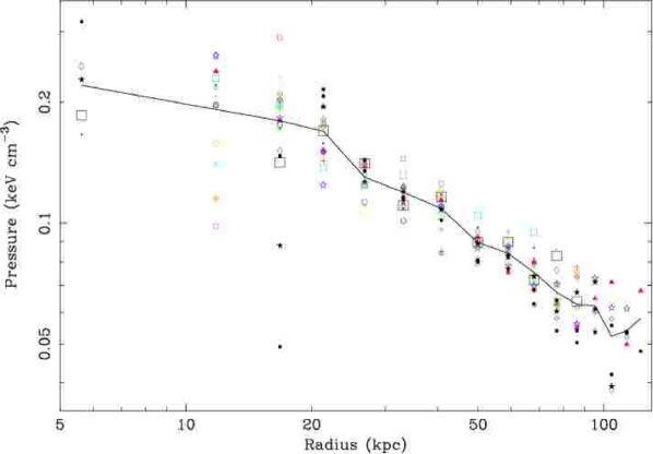
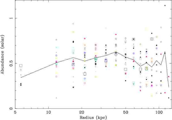
Figure 21: Combined radial profiles of the values in Fig. 18 and Fig. 19. Each sector is marked by its own unique plot symbol. The mean profiles are shown by the lines. The outermost points in each sector are not plotted. The radii shown are the mean radii for individual sectors.

In Fig. 21 are shown radial plots containing the values for all of the sectors. The values in each sector generally vary smoothly from annulus to annulus, except in the centre and at the position of the outer NW radio lobe. In addition, although there is variation from sector to sector, the sectors appear to follow the same trends. There are some regions for which the entropy appears to increase inwards away from the lobes and the cold rims (e.g. 230 arcsec from the core to the SE), suggesting there are convectively unstable volumes in the core. In these plots we do not plot the outermost sectors as the density is overestimated as we cannot subtract the contribution from gas that lies outside that sector, nor do we plot points were the projection model fails.

We can plot the temperatures of individual bins against their entropies (Fig. 22 [top]). The distribution is well fit with the relation $S=1.5(kT)^{2.5}$, with $S$ in $\rm\thinspace keV\rm\thinspace cm^{2}\,$ and $kT$ in keV. There appear to be separate clumps of points in the plot which are separate in temperature.

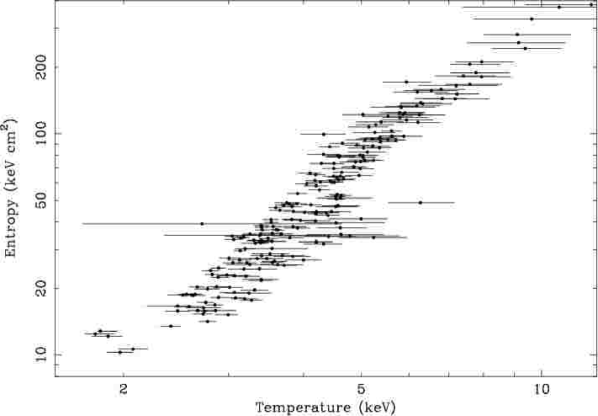
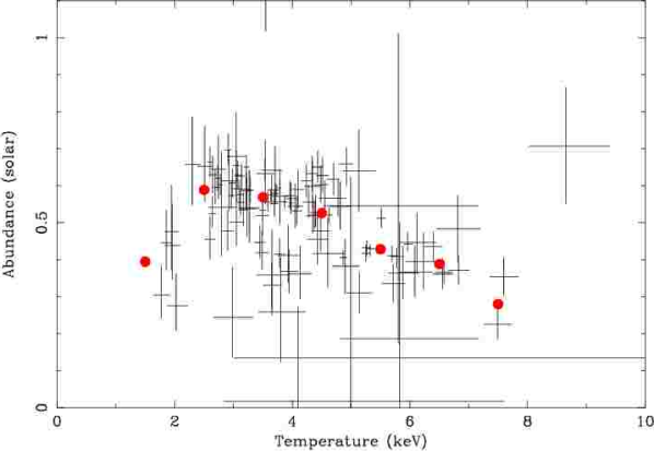
Figure 22: (Top) Entropy of the partial-annuli in Fig. 18 plotted against the temperature. Outer annuli, and sectors occupied by the radio lobes or where projection failed were excluded. (Bottom) Abundance of each partial-annulus plotted against its temperature. The solid points mark the weighted mean abundance in 1 keV bins between 1 and 8 keV. Fewer radial sectors were used to create this plot than in the rest of this section, reducing the uncertainties on the abundance measurements.

In Fig. 19 (right) we plot the abundances of each of the sectors. There is a reasonable correspondence with the projected abundance map in Fig. 10. The abundance profile peaks away from the centre like the projected abundance (Fig. 21), although the points are more noisy. We can also plot the abundance of sectors against their temperature (Fig. 22 [bottom]) to test the projected relation in Fig. 11. Although the abundances have larger uncertainties, when they are averaged in temperature bins, we see a similar relation to Fig. 11, but with a dip in abundance at low temperatures.

It is physically interesting to plot the quantity of gas present as a function of temperature, which we can compare to what would be expected from a standard cooling flow, and as a function of abundance. Fig. 23 shows these distributions, calculated using the temperatures, densities and abundances from Fig. 21. Sectors in which the emission measures were consistent with being zero were ignored in this analysis. On the temperature-mass plot we plot a line representing the amount of mass we would expect as a function of temperature in an isobaric cooling flow, with the mass deposition rate $\dot{M}=300\hbox{$\hbox{$\rm\thinspace M_{\odot}$}\rm\thinspace yr^{-1}\,$}$, the pressure $P=n_{e}T=5\times 10^{5}\hbox{$\rm\thinspace K\rm\thinspace cm^{-3}\,$}$, and abundance $0.4\hbox{$\thinspace\mathrm{Z}_{\odot}$}$. The amount of mass in a temperature interval, $\Delta M\propto\dot{M}/(P\Lambda)$. Increasing the abundance or pressure (which can be functions of temperature) will decrease the mass in a temperature interval.

Gas is fairly uniformly distributed by mass over a factor of 3 range in temperature, from 2.5 to 8 keV, with little gas detected below 2 keV. The shape of this observed distribution is the essence of the ‘cooling flow problem’ (Peterson et al. 2003; Fabian 2003).

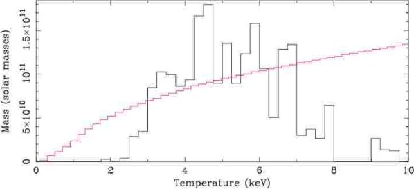
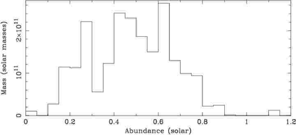
Figure 23: The gas mass as a function of temperature (summed in 0.25 keV bins), and as a function of abundance (in $0.05\hbox{$\thinspace\mathrm{Z}_{\odot}$}$ bins), computed from Fig. 18 and Fig. 19 (right). The dotted line on the temperature plot shows the distribution as expected in a cooling flow with $\dot{M}=300\hbox{$\hbox{$\rm\thinspace M_{\odot}$}\rm\thinspace yr^{-1}\,$}$, $P=5\times 10^{5}\hbox{$\rm\thinspace K\rm\thinspace cm^{-3}\,$}$ and $Z=0.4\hbox{$\thinspace\mathrm{Z}_{\odot}$}$.

8.2 Fitting individual abundances

We fit vmekal models with variable abundances to the spectra extracted from partial-annuli, accounting for projection, and using the whole band 0.6 to 8 keV. We divided the cluster up into only four equal sectors, starting the first sector $25^{\circ}$ to the NW from the N. The model was fit to the whole band, and the O, Ne, Mg, Si, S, Ar, Ca, Fe and Ni abundances were thawed. The Ni, Mg, Si and S abundances may be contaminated with the residuals near 2 keV. Fig. 24 shows the elemental abundance profiles, produced by taking the best fitting values in the four sectors, and computing a weighted mean of the values. This procedure was done to allow for the variation in temperature in each sector. The uncertainties of each point are the uncertainties on the weighted mean. The uncertainties on the best fitting abundances were symmetrised using the RMS uncertainty. Any sectors where the temperature was compatible with less than 1 or greater than 14 keV were excluded. The Ni and Mg results using a vapec model are also shown. Ni abundances are substantially smaller using this model. The Fe plot also shows a profile only using the Fe-K lines. The central values should be taken with caution as the deprojection analysis appears to fail in three of the four sectors.

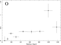
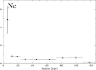
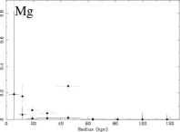
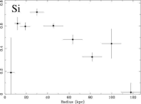
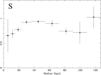
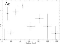
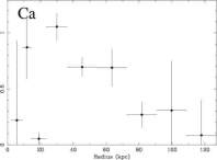
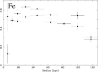
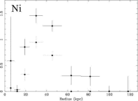
Figure 24: Average abundance profile in the four sectors, produced by fitting the full 0.6-8 keV band with a vmekal model accounting for projection. The values are the weighted mean of the four sectors (symmetrising uncertainties on the sectors and excluding any sectors where the temperature is undefined) The uncertainties on the points are the uncertainty on the mean. The dotted points on the Ni and Mg plots show the results using a vapec model, and the dotted points on the Fe plot show the Fe-K abundances.

The fact that the Si, S, Ar, Ca, Fe and Ni profiles all drop in the centre of the cluster strongly suggest that ‘Fe-bias’ is not the cause of the decrease.

8.3 Multiple temperature components

A simple test for the presence of multiple temperature components is to add a component at one half of a fitted temperature. It is difficult to distinguish a temperature component less than a factor of two away. In Fig. 25 we show the probability that the improvement in $\chi^{2}$ obtained in adding a second component is purely due to chance. The plot was generated by fitting a single temperature model to each annulus, accounting for projection, measuring $\chi^{2}$ of the fit, and then adding a second component, and again measuring $\chi^{2}$. Then the F-statistic was generated and used to find the probability. Annuli outside the annulus being fitted always have two components, so the probability is purely measured in the annulus.

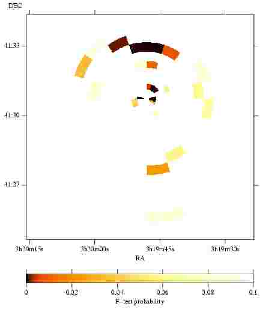
Figure 25: F-test probability of improvement of $\chi^{2}$ given by second component being by chance.

We find that there is not a substantial improvement of $\chi^{2}$ given by multiple temperature fits, except on the N rim of the radio lobe (which is spatially narrower than the bin used), and to the W of the nucleus.

We also repeated the multiple temperature component analysis of Section 7 accounting for projection in six sectors. The results from the two sets of analyses appear to be quite similar, so we do not show the versions accounting for projection here. In the 0.5 keV plot there is a low level of gas over much of the core, but more at the centre. In the 1 keV plot there is little evidence for gas at that temperature, except right in the core and in the outer regions. At 2 and 4 keV, the cool swirl we see in the projected map is seen again. At 8 keV the outer parts of the core are visible, and there is some apparent presence of gas near the centre. At 16 keV there are some differences between the projected map and the map we present here. Accounting for projection, we do not see gas near 16 keV as extensively distributed to the N of core, but we do see it to the S in the outer regions. If we examine the abundances produced using this analysis, the Ni and Fe abundances still appear to drop towards the centre in several sectors.

Additionally, if we perform the same analysis as in Section 8.2 but adding a second temperature component at half of the fitted temperature, none of the profiles look substantially different to the single temperature results.

9 Radio lobes

We examined the X-ray emission in detail from the features associated with the radio lobes, using the projct model in xspec to account for projection effects. Spectra were extracted from sectors moving out from the radio lobes. We examined the inner SW, NE, and outer S and NW radio lobes. Early work on the filling factor of the holes using the 25 ks dataset was reported by Schmidt et al (2002).

We found that this simple deprojection analysis failed. There was too little emission from the inner SW, NE and outer NE lobe regions than would be expected from the projected emission of overlying gas, assuming spherical symmetry in the sectors. Fig. 26 shows the projected spectrum of the inner SW radio lobe (points). The upper line in the plot is the expected projected emission from the region if the lobe itself were void. Since we found less emission than we excepted from projection, there is an enhancement outside the lobes on the plane of the sky which is not present along the line of sight. This effect may simply be due to the radio lobes displacing the hot gas outward, so leading to excess emission beyond the lobes. To account for this difference, we fit the deficit in emission in the SW lobe with a thermal spectrum, resulting as the reduced prediction shown as the lower line in Fig. 26. The temperature of the thermal component is $\sim 3$ keV. In contrast, there is more soft emission in the outer S lobe than would be expected by projection. Taking into account these soft components, we find little evidence for any emission from the radio lobes themselves.

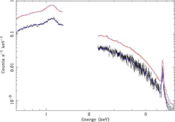
Figure 26: The points show a spectrum extracted from the inner SW radio lobe. The upper line shows a model for the spectrum assuming there is no emission from the radio lobe, and the only contribution is projected emission (assuming spherical symmetry in a sector). The lower line shows the same model, but reduced by a mekal component to account for the excess emission on the plane of the sky.

The radio spectral index in the region of the SW lobe is about unity (Fabian et al 2002) and the 330 MHz radio luminosity about $3\times 10^{39}\hbox{$\rm\thinspace erg\rm\thinspace s^{-1}\,$}$ from the maps of Pedlar et al (1990). This is considerably smaller than our limit for deprojected power-law X-ray emission with the same spectral index of about $2\times 10^{43}\hbox{$\rm\thinspace erg\rm\thinspace s^{-1}\,$}$ (once the 3 keV soft component is taken into account). The radio to X-ray luminosities should be roughly in the ratio of the energy density in the magnetic field to that in the cosmic microwave background (assumed to be source of target photons for inverse Compton scattering). This gives a lower limit on the magnetic field of $B>10^{-7}$ G, much less than the likely field of $10^{-5}$ G (Fabian et al 2002). Reworking this result using the formulae of Harris & Grindlay (1979) gives a limit about 1.5 times smaller. This means that our current X-ray observations are far from detecting the inverse Compton emission, mainly due to the brightness of the thermal gas.

10 Discussion

10.1 Temperature structure

The high resolution images of the projected emission-weighted temperature in Section 5, illustrate that there is a considerable wealth of temperature structure in the cluster. There is a factor of 4.3 in projected temperature between the coolest gas we observe (2.4 keV) to the hottest (10.3 keV). If we take the coolest blob and use a neighbouring region as a background spectrum, the best fitting temperature is $1.45^{+0.28}_{-0.06}$ keV. This is comparable with the temperature of the X-ray emission associated with the H$\alpha$ filaments (Fabian et al 2003b).

Accounting for projection effects (Fig. 21), we observe the gas near the nucleus goes down to $\sim 1.8\rm\thinspace keV$ (although spherical symmetry assumptions fail very close to the central object). The shortest radiative cooling time we measure in this analysis is around 0.18 Gyr (although if we underestimated the abundance of material in the core, this period will be shorter).

Looking at the results from the multiple temperature component analysis (Fig. 15), then there may be some gas, especially near the core, at temperatures near 0.5 keV with a low VFF. There may be a significant amount of gas near 1 keV around the nucleus too. Surprisingly, the gas at 0.5 keV appears to take up more volume than that at 1 keV. These results, particularly the surprising 0.5 keV map, depend on there not being significant systematics there. Once the response below 0.6 keV is more accurately determined we will be able to confirm whether gas is at these temperatures. If there is gas at low temperatures then this may indicate there could be gas cooling, but at rates reduced from earlier studies.

Another surprising result from fitting multiple temperature components is the existence of a band of gas near 8 keV to the N of the nucleus. Some of the band coincides with the position of the HVS, but it is more extensive. It would be surprising if this were shocked gas from the HVS given its VFF and extent. Although we do have limited spatial resolution, some of the band appears coincident with the weak shock identified to the NE (Fabian et al 2003a). The remainder of this gas appears to be within this radius, so it is possible we are observing post-shocked gas.

The 16 keV map is difficult to interpret. It is not uniform, so is unlikely to be due to incomplete background subtraction. In addition there is no indication of emission where the gas is the hottest, especially to the SE corner of the map. It may still be a background effect if there are other significant systematics, but reassuringly the count rate in a 10 to 12 keV band agrees with the rate in the blank-sky observation we have used for background spectra to 2 per cent. The most probable explanation is that there is diffuse non-thermal emission over the cluster core. The morphology of this emission is not matched to the radio lobes, although at the location of the radio lobes there appears to be emission. If this is non-thermal emission, rather than some sort of unidentified systematic uncertainty, then it could be due to a different population of particles to those producing the radio lobes. It may, for instance, be associated with the radio mini halo in the Perseus core (Pedlar 1990; see also Fabian & Kembhavi 1982; Gitti, Brunetti & Setti 2002). The radio mini halo does have some morphological resemblance to the region where the 16 keV component is strongest. The presence of a hard component over the inner region of the Perseus cluster and other nearby clusters had also been indicated by previous ASCA observations (Allen et al 2001).

In Fig. 27 we show the individual temperature component contributions to a multi-component fit of the entire ACIS-S3 spectrum. If we replace the 16 keV component with a more physically relevant power-law component (which incidentally gives a better fit to the spectrum), then the best-fitting power-law index is 1.3, and its luminosity is $3.3\times 10^{43}\hbox{$\rm\thinspace erg\rm\thinspace s^{-1}\,$}$ in the 1 to 10 keV band. This luminosity is around three times greater than the luminosity of the nucleus as reported by Churazov et al (2003a; agreeing with the luminosity calculated from our moderately piled-up spectrum of the central source). The $\chi^{2}$ of the fit reduces by around 200 with a hard component present. Future X-ray missions, such as ASTRO-E2, will be able to easily detect this hard-component if it is not due to background effects.

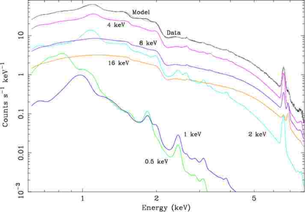
Figure 27: The contributions of the temperature components to the muli-temperature model, which is shown in grey. The model was fitted to the total ACIS-S3 spectrum, which is plotted in black beneath the total model. The spectrum contains $1.5\times 10^{7}$ counts.

10.2 Absorption structure

A basic interpretation of Fig. 6 would indicate there could be evidence of absorbing material associated with the coolest gas. Unfortunately this may be a result of either instrument calibration, and the low energy QE degradation.

10.3 Abundance structure

The metallicity of the cores of cooling flow clusters has long been known to differ from the outer parts of the same clusters. An iron metallicity gradient is often observed (Fukazawa et al 1994; Allen & Fabian 1998; Irwin & Bregman 2001; De Grandi & Molendi 2001). Chandra data sometimes reveals that it drops again in the centre (Sanders & Fabian 2002; Johnstone et al 2002; Schmidt et al 2002; Blanton, Sarazin & McNamara 2003). The behaviour of the abundances of other elements is not straightforward (e.g. Tamura et al 2001; Finoguenov et al 2002; Ettori et al 2002), with oxygen showing little change across the core and nickel showing a strong excess (Dupke & Arnaud 2001).

A general picture was established of Type II supernovae dominating the bulk of the gas (especially the outer gas) and the central abundance peak being dominated by Type Ia supernovae. The details of the observations do not however fit completely with such a simple picture and consideration has been made of an early population of hypernovae contributing to all the gas (e.g. Loewenstein 2001) and of there being different classes of Type Ia events (see Baumgartner et al 2003 and Loewenstein 2003 for an overall discussion of all supernova types). Other issues that could be relevant here are an ‘Fe bias’ due to the gas really being multiphase but treated as single-phase (Buote & Fabian 1998; Buote 1999), rapid cooling of metal-rich regions (Fabian et al 2001; Morris & Fabian 2003), sedimentation of metals (Fabian & Pringle 1977; Gilfanov & Syunyaev 1984), resonance-line scattering (Gilfanov et al 1987), gas flows (Fabian 2003) and photoionization by the central active nucleus.

We find in Perseus that O and Mg (perhaps our most unreliable measurements) show no central peak whereas Fe, Si, S, Ca and Ni show an off-centre peak. Ne is the only element which peaks at the centre. Ni reaches the highest metallicity which is plausibly an indication of strong Type Ia enhancement from the central galaxy NGC 1275. The peaks in Si and S may indicate that the Type Ia events produce significant quantities of Si and S, although a combination of Type Ia and II may be more relevant. Given that the spectrum of the body of NGC 1275 is, despite being a giant elliptical, of spectral type A, then a steady occurrence of supernovae are expected, of both Type Ia and II (SN 1968A in NGC 1275 was of Type I; Barbon, Cappellaro & Turatto 1989; Meusinger & Brunzendorf 1996; Capetti 2002). The central Ne peak unexpected, but it should be noted that the Ne-K lines occur within the band containing the Fe-L lines so some spectral confusion could occur if the temperature structure of the gas is not simple. (Ettori et al 2002 find a broad central Ne peak in A 1795.)

The abundances and radial trends we find, ignoring Mg, are very similar to those found in M87 (Finoguenov et al 2002; Gastaldello & Molendi 2002; Matsushita, Finoguenov & Böhringer 2003). Si however is more abundant in M87, peaking at a value about twice that found here in Perseus. The overall agreement is impressive given that the temperatures in Perseus are 2.5 – 3 times those at the same radius in M87. The ratio S/Si is about 1.5 in Perseus but less than one in M87. Matsushita et al (2003) argue for a significant Si contribution from SN Ia.

The excess mass of iron in the inner 70 kpc of the Perseus cluster is about $2\times 10^{8}\hbox{$\rm\thinspace M_{\odot}$}$. Excess here means exceeding a metallicity of 0.4. The similar mass for M87 is $7\times 10^{7}\hbox{$\rm\thinspace M_{\odot}$}$. The 2MASS total $J$ magnitudes of the two galaxies indicate that NGC 1275 is about 1.6 times the stellar mass of M87, whereas the excess iron masses differ by a factor of three. The overall difference may be due to continued supernova activity in NGC 1275.

Resonance scattering (Gilfanov et al 1987) has been ruled out for the bulk of the Fe-K line emission in the Perseus cluster by studies of the Fe-K$\alpha$/K$\beta$ ratio with XMM-Newton (Churazov et al 2003b; Gastaldello & Molendi 2003). Mild motions of the intracluster medium can account for this. Nevertheless, it is possible that the central emission and some of the L-shell lines are still thick to resonance scattering.

This could account for the central differences in Fe-K and Fe-L abundance measurements and indeed for the general drop in central abundances. The central Ne peak may be an indication that resonance scattering is affecting the Fe-L emission at the centre, in the following manner. The expected Ne X emission (12.2A) coincides with non-resonant L-shell emission from FeXXIII and FeXXII. If the Fe-L resonance lines from FeXXIV and FeXXIII (at 10.6, 11, 11.4 and 11.8A) are significantly scattered near the centre then we fit an artificially low iron abundance to that region. Emission at 12.2A is then wrongly attributed to Ne. In other words, the present evidence supports a resonance scattering interpretation of the apparent central drop in metal abundances from many species. The apparent peak in Ne is due to Fe-L not Ne. Spectral fitting of projected spectra in the central regions show that this hypothesis is tenable. We shall pursue these issues in detail elsewhere.

Finally, we note the similarity of our mean abundance-temperature values (Fig. 22 [bottom]) of the gas in the core of the Perseus cluster with those of the large ASCA sample studied by Baumgartner et al (2003; their Fig. 2). They eliminated the brightest clusters from this plot and also were usually measuring the whole observed cluster. This suggests a universal $Z-kT$ relation which would be very puzzling. However, the Centaurus cluster and M87 have profiles which, although of similar shape, are both stronger and shifted to lower temperatures. There is not therefore a fixed universal profile, although the peaked shape seems to be universal. An overall summary is that most cluster gas which is above 6 keV has a metallicity below about 0.3, whereas most gas at 3 keV has a metallicity (iron) of 0.4 or higher. At the lowest temperatures observed the metallicity drops to 0.2 or less. We do not understand this result.

11 Conclusions

We have studied a 191 ks Chandra image of the core of the Perseus cluster for small-scale temperature and abundance structures. The obvious X-ray surface brightness features are seen to be due to temperature variations, with corresponding density variations ensuring approximate azimuthal pressure balance. Such variations are seen on scales down to above 2.5 arcsec ($\sim 1$ kpc) in the brightest regions.

We have made extensive searches for multi-temperature gas components. There is little evidence in the deprojected spectra for any widespread components at a temperature more than a factor of two away from the local temperature. There is some evidence for a widespread hot component (at 16 keV) in the projected data. This emission could alternatively be due to an extended nonthermal component. The solution to the cooling flow problem in the Perseus cluster must produce a fairly uniform mass distribution of gas from 2.5 to 8 keV, with little gas below 2 keV.

The abundances of Si, S, Ar, Ca, Fe and Ni rise inward from about 100 kpc, peaking at about 30–40 kpc. Most of these abundances level out or drop again inward of the peak. The extent of the drop is unclear, but it is plausibly explained by resonance scattering. O and Mg are more uniform across the core and Ne shows a central peak. The overall abundance pattern is similar to that found by others using XMM-Newton data of M87 in the Virgo cluster, except that S/Si exceeds unity in the Perseus cluster core. The abundance peaks are likely due to Type Ia supernovae in the central galaxy, NGC 1275.

References

- [1] Allen S.W., Fabian A.C., 1998, MNRAS, 297, L63
- [2] Allen S.W., Fabian A.C., Johnstone R.M., Arnaud K.A., Nulsen P.E.J., 2001, MNRAS, 322, 589
- [3] Anders E., Grevesse N., 1989, Geochimica et Cosmochimica Acta, 53, 197
- [4] Arnaud, K.A., 1996, Astronomical Data Analysis Software and Systems V, eds. Jacoby G. and Barnes J., p17, ASP Conf. Series volume 101
- [5] Balucinska-Church M., McCammon D., 1992, ApJ, 400, 699
- [6] Barbon R., Cappellaro E., Turatto M., 1989, A&AS, 81, 421
- [7] Baumgartner W.H., Loewenstein M., Horner D.J., Mushotzky R.F., 2003, ApJ, submitted, astro-ph/0309166
- [8] Blanton E.L., Sarazin C.L., McNamara B.R., 2003, ApJ, 585, 227
- [9] Böhringer H., Voges W., Fabian A.C., Edge A.C., Neumann D.M., 1993, MNRAS, 264, L25
- [10] Buote D.A., Fabian A.C., 1998, MNRAS, 296, 977
- [11] Buote D.A., 1999, MNRAS, 309, 685
- [12] Buote D.A., 2000, ApJ, 539, 172
- [13] Cappellari M., Copin Y., 2003, MNRAS, 342, 345
- [14] Capetti A., 2002, ApJ, 574, L25
- [15] Cash W., 1979, ApJ, 228, 939
- [16] Chartas G., Getman K., 2002, http://www.astro.psu.edu/users/chartas/xcontdir/xcont.html
- [17] Churazov E., Forman W., Jones C., Böhringer H., 2000, A&A, 356, 788
- [18] Churazov E., Forman W., Jones C., Böhringer H., 2003a, ApJ, 590, 225
- [19] Churazov E., Forman W., Jones C., Sunyaev R., Böhringer H., 2003b, ApJ, in press, astro-ph/0309427
- [20] De Grandi S., Molendi S., 2001, ApJ, 551, 153
- [21] Dickey J.M., Lockman F.J., 1990, ARA&A, 28, 215
- [22] Dupke R.A., Arnaud K.A., 2001, ApJ, 548, 141
- [23] Dupke R.A., Bregman J.N., 2001, ApJ, 547, 705
- [24] Ettori S., Fabian A.C., Allen S.W., Johnstone R.M., 2002, MNRAS, 331, 635
- [25] Fabian A.C., Pringle J.E., 1977, MNRAS, 181, 5
- [26] Fabian A.C., Kembhavi A., 1982, in Proc IAU Symp 97,, eds D.S. Heeschen, C.M. Wade, Reidel Dordrecht p453
- [27] Fabian A.C., 1994, A&AR, 32, 277
- [28] Fabian A.C., Mushotzky R.F., Nulsen P.E.J., Peterson J.R., 2001, MNRAS, 321, L20
- [29] Fabian A.C., Celotti A., Blundell K.M., Kassim N.E., Perley R.A., 2002, MNRAS, 331, 369
- [30] Fabian A.C., Sanders J.S., Ettori S., Taylor G.B., Allen S.W., Crawford C.S., Iwasawa K., Johnstone R.M., Ogle P.M., 2000, MNRAS, 318, L65
- [31] Fabian A.C., Sanders J.S., Allen S.W., Crawford C.S., Iwasawa K., Johnstone R.M., Schmidt R.W., Taylor G.B., 2003a, MNRAS, 344, L43
- [32] Fabian A.C., Sanders J.S., Crawford C.S., Conselice C.J., Gallagher III J.S., Wyse R.F.G., 2003b, MNRAS, 344, L48
- [33] Fabian A.C., 2003, MNRAS, 344, L27
- [34] Finoguenov A., Matsushita K., Böhringer H., Ikebe Y., Arnaud M., 2002, A&A, 381, 21
- [35] Fukazawa Y., Ohashi T., Fabian A.C., Canizares C.R., Ikebe Y., Makishima K., Mushotzky R.F., Yamashita K., 1994, PASJ, 46, L55
- [36] Gastaldello F., Molendi S., 2002, ApJ, 572, 160
- [37] Gastaldello F., Molendi S., 2003, ApJ, in press, astro-ph/0309582
- [38] Gilfanov M.R., Syunyaev R.A., 1984, Soviet Astr. Lett., 10, 137
- [39] Gilfanov M.R., Syunyaev R.A., Churazov E.M., 1987, Soviet Astr. Lett., 13, 233
- [40] Gillmon K., Sanders J.S., Fabian A.C., 2003, MNRAS, in press
- [41] Gitti M., Brunetti G., Setti G., 2002, A&A, 386, 456
- [42] Harris D.E., Grindlay J.E., 1979, MNRAS, 188, 25
- [43] Irwin J.A., Bregman J.N., 2001, ApJ, 546, 150
- [44] Johnstone R.M., Fabian A.C., Edge A.C., Thomas P.A., 1992, MNRAS, 255, 431
- [45] Johnstone R.M., Allen S.W., Fabian A.C., Sanders J.S., 2002, MNRAS, 336, 299
- [46] Liedahl D.A., Osterheld A.L., Goldstein W.H., 1995, ApJ, 438, L115
- [47] Loewenstein M., 2001, ApJ, 557, 573
- [48] Loewenstein M., 2003, to appear in Carnegie Observatories Astrophysics Series, Vol. 4: Origin and Evolution of the Elements, ed. A. McWilliam, M. Rauch, CUP, astro-ph/0310557
- [49] Marshall H.L., Tennant A., Grant C.E., Hitchcock A.P., O’Dell S., Plucinsky P.P., 2003, proc. SPIE, in press, astro-ph/0308332
- [50] Matsushita K., Finoguenov A., Böhringer H., 2003, A&A, 401, 443
- [51] Meusinger H., Brunzendorf J., 1996, proc. ‘Röntgenstrahlung from the Universe’, eds. Zimmermann, H.U.; Trümper, J.; and Yorke, H.; MPE Report 263, p. 599-600
- [52] Mewe R., Gronenschild E.H.B.M., van den Oord G.H.J., 1985, A&AS, 62, 197
- [53] Morris R.G., Fabian A.C., 2003, MNRAS, 338, 824
- [54] Pedlar A., Ghataure H.S., Davies R.D., Harrison B.A., Perley R., Crane P.C., Unger S.W., 1990, MNRAS, 246, 477
- [55] Peterson J.R. et al., 2001, A&A, 365, L104
- [56] Peterson J.R., Kahn S.M., Paerels F.B.S., Kaastra J.S., Tamura T., Bleeker J.A.M., Ferrigno C., Jernigan J.G., 2003, ApJ, 590, 207
- [57] Sanders J.S., Fabian A.C., 2002, MNRAS, 331, 273
- [58] Schmidt R.W., Fabian A.C., Sanders J.S., 2002, MNRAS, 337, 71
- [59] Smith R.K., Brickhouse N.S., Liedahl D.A., Raymond J.C., 2001, ApJ, 556, L91
- [60] Tamura T., Bleeker J.A.M., Kaastra J.S., Ferrigno C., Molendi S., 2001, A&A, 379, 107
- [61] Vikhlinin A., 2002, http://hea-www.harvard.edu/alexey/corrarf/
- [62] Vikhlinin A., 2003, http://asc.harvard.edu/cont-soft/software/corr_tgain.1.0.html