IRFM $T_{\mathrm{eff}}$ calibrations for cluster and field giants in the Vilnius, Geneva, $RI_{\mathrm{(C)}}$ and DDO photometric systems

Based on a large sample of disk and halo giant stars, for which accurate effective temperatures derived through the InfraRed Flux Method (IRFM) exist, a calibration of the temperature scale in the Vilnius, Geneva, $RI_{\mathrm{(C)}}$ and DDO photometric systems is performed. We provide calibration formulae for the metallicity dependent $T_{\mathrm{eff}}$ vs color relations as well as grids of intrinsic colors and compare them with other calibrations. Photometry, atmospheric parameters and reddening corrections for the stars of the sample have been updated with respect to the original sources in order to reduce the dispersion of the fits. Application of our results to Arcturus leads to an effective temperature in excellent agreement with the value derived from its angular diameter and integrated flux. The effects of gravity on these $T_{\mathrm{eff}}$ vs color relations are also explored by taking into account our previous results for dwarf stars.

1 Introduction

In a previous paper (Meléndez & Ramírez melendez03 (2003), Paper I) we derived $T_{\mathrm{eff}}:$ color $:\mathrm{[Fe/H]}$ relations for dwarf stars in the Vilnius, Geneva, $RI_{\mathrm{(C)}}$ and DDO systems from the Alonso et al. (1996a ) sample. This time, we have performed a similar extension for giants by using the corresponding Alonso et al. (1999a ) sample. We have chosen this sample in order to maintain the homogeneity of the calibrations, the effective temperatures of all of the stars in both samples (dwarfs and giants) have been obtained in a single implementation of the InfraRed Flux Method (IRFM) by Alonso and coworkers.

In addition to their primary importance as fundamental relations, these empirical $T_{\mathrm{eff}}$ calibrations are extremely useful for several purposes. Applications include chemical abundance studies (e.g. Smith et al. smith02 (2002), Kraft & Ivans kraft03 (2003)), the transformation of theoretical HR diagrams into their observational counterparts, i.e. color-magnitude planes (e.g. Girardi et al. girardi02 (2002)) and the test of synthetic spectra and colors (e.g. Bell bell97 (1997)). When used along with other studies, combined results may have implications in galactic chemical evolution, population synthesis and cosmology.

A noteworthy feature of our work and that of Alonso et al. (1996b , 1999b ) is the inclusion of Population II stars in the calibrations. They allow to extend the ranges of applicability of the formulae, which in turn become useful also for metal-poor stars. In order to achieve this goal, a large number of cluster giants has been included in the sample adopted for the present work. Even though for a given photometric system observations are usually available for only 2 or 3 clusters, the number of stars contributed by each of them is considerable and thus deserved to be included.

When comparing temperature scales of main sequence stars with those corresponding to giants, small but systematic differences arise. Theoretical calculations can easily take into account these variations with the $\log g$ value. In empirical studies, however, it is only after a considerable number of stars has been studied and their properties properly averaged that gravity effects become clear. Detailed, careful inspection of gravity effects on colors may improve our understanding of the physics behind stellar spectra formation.

The present work is distributed as follows: Sect. 2 describes the data adopted, in Sect. 3 we discuss some properties of the general calibration formula employed, perform the calibrations and apply them to Arcturus. Comparison of our work with previously published calibrations is presented in Sect. 4 while intrinsic colors of giant stars and the effects of gravity on the temperature scale are discussed in Sect. 5. We finally summarize our results in Sect. 6.

2 Photometry and atmospheric parameters adopted

Colors adopted in this work were obtained from the General Catalogue of Photometric Data (GCDP, Mermilliod et al. mermilliod97 (1997)), as in Paper I. Nevertheless, due to the lack of $RI_{\mathrm{(C)}}$ photometry for giants, colors obtained by applying transformation equations to Kron-Eggen and Washington photometry were also adopted, as explained in Sect. 3.3.

The reddening corrections $E(B-V)$ are given in the work of Alonso et al. (1999a ). For most of the stars in globular clusters, however, these values have been updated following Kraft & Ivans (kraft03 (2003), KI03). Although reddening ratios $E(\mathrm{color})/E(B-V)$ for medium and broad band systems generally depend on spectral type, their variations with luminosity class for our interval of interest (F5-K5) amount to a maximum of 0.05 and so only relevant values have been changed with respect to the values adopted for dwarfs. Thus, for giants we have taken $E(Z-V)/E(B-V)=0.30$ and $E(Y-Z)/E(B-V)=0.54$ (Straižys straizys95 (1995)). The reddening ratio $E(B_{1}-B_{2})/E(B-V)=0.35$ (Cramer cramer99 (1999)) was also necessary to obtain intrinsic $t$ parameters in the Geneva system (Sect. 3.2). For the remaining colors, the adopted reddening ratios are the same as those given in Paper I (see our Table 1 and references therein).

Several stars were discarded before performing the fits due to their anomalous positions in $T_{\mathrm{eff}}$ vs color planes. It is worth mentioning the most discrepant of them and the probable causes of this behaviour (temperatures are those given by Alonso et al. 1999a ): BD +11 2998, noted by Alonso et al. (1999a ) as a “probable misindentification in the program of near IR photometry”, an F8 star with very high $T_{\mathrm{eff}}=7073$ K; and BS 2557, also HD 50420, a blue A9III variable star, $T_{\mathrm{eff}}=4871$ K.

Regarding $\mathrm{[Fe/H]}$ values, the catalogue of Cayrel de Strobel et al. (cayrel92 (1992)) has been superseded by the 2001 edition (Cayrel de Strobel et al. cayrel01 (2001)). In addition, we have updated the 2001 catalogue from several abundance studies, introducing more than 1000 entries and 357 stars not included in the original catalogue. The most important sources for this update were: Mishenina & Kovtyukh (mishenina01 (2001)), Santos et al. (santos01 (2001)), Heiter & Luck (heiter03 (2003)), Stephens & Boesgaard (stephens02 (2002)), Takada-Hiday et al. (takada02 (2002)) and Yong & Lambert (yong03 (2003)). We will call “C03” this actualized catalogue.

Hilker (hilker00 (2000), H00) has published a metallicity calibration for giants in the Strömgren system, which, when compared with the spectroscopic metallicities of C03 shows clear systematic tendencies (Fig. 1). The systematic difference between H00 and C03 fit approximately the following empirical relation: $\mathrm{[Fe/H]}_{\mathrm{H00}}-\mathrm{[Fe/H]}_{\mathrm{C03}}=0.274\mathrm{[Fe/H]}^{2}+0.511\mathrm{[Fe/H]}-0.002$, which is also shown in Fig. 1 as a dotted line. By substracting this difference from the $\mathrm{[Fe/H]}$ values obtained from the H00 calibration we obtain a modified H00 metallicity in better agreement with C03.

Figure 1: Upper panel: Differences between photometric $\mathrm{[Fe/H]}$ values from the Hilker (hilker00 (2000), H00) calibration and C03 spectroscopic determinations for a subsample of giant stars. Bottom panel: Differences between the modified photometric $\mathrm{[Fe/H]}$ values [H00(m)] and C03 spectroscopic determinations.

We have adopted $\mathrm{[Fe/H]}$ values in order of reliability: firstly C03 values ($\sim 70\%$ of the sample), secondly the modified Hilker (hilker00 (2000)) calibration ($\sim 5\%$) and lastly the photometric metallicities given by Alonso et al. (1999a ).

3 The calibrations

Broadly speaking, the behaviour of the $T_{\mathrm{eff}}$ vs color relations can be represented by the simple equation: $T_{\mathrm{eff}}=c_{1}/(c_{2}\mathrm{X}+c_{3})$, where X is the color index and $c_{1}$, $c_{2}$ and $c_{3}$ constants (see for example Hauck & Künzli hauck96 (1996)). It is easy to show, by aproximating the stellar flux to that of a blackbody, that this equation has some physical meaning. To better reproduce the observed gradients $\Delta T_{\mathrm{eff}}/\Delta\mathrm{X}$ and to take into account the effects of different chemical compositions, however, the following general formula has proved to be more accurate:

$$\theta_{\mathrm{eff}} = a_{0}+a_{1}\mathrm{X}+a_{2}\mathrm{X}^{2}+a_{3}\mathrm{X}\mathrm{[Fe/H]}$$ (1)

$$+a_{4}\mathrm{[Fe/H]}+a_{5}\mathrm{[Fe/H]}^{2}\ .$$

Here, $\theta_{\mathrm{eff}}=5040/T_{\mathrm{eff}}$ and $a_{i}$ ($i=0,1,\ldots,5$) are the constants of the fit (see for example Alonso et al. 1996b , 1999b ; Meléndez & Ramírez melendez03 (2003)).

Nonlinear fits of the data to Eq. (1) were performed for 7 color indices and 1 photometric parameter as described in the following subsections. Coefficients such that $3\sigma(a_{i})>a_{i}$ were neglected and stars departing more than $2.5\sigma(T_{\mathrm{eff}})$ from the mean fit where iteratively discarded (the number of iterations hardly exceeded 5).

It has been argued that the $a_{5}$ term, which is almost always negative, systematically produces too high temperatures for metal-poor stars (Ryan et al. ryan99 (1999), Nissen et al. nissen02 (2002)). For a non-negligible $a_{5}$ term, the dependence of $T_{\mathrm{eff}}$ on $\mathrm{[Fe/H]}$ gradually increases as very low values of $\mathrm{[Fe/H]}$ are considered. Physically, this is not an expected behaviour since $T_{\mathrm{eff}}$ should become nearly independent of $\mathrm{[Fe/H]}$ as less metals are present in the stellar atmosphere. We have carefully checked the residuals of every iteration in order to reduce this kind of tendencies, specially for the $-3.0<\mathrm{[Fe/H]}\leq-2.5$ group, and have made $a_{5}=0$ when necessary.

Even after these considerations, the residuals of some fits showed systematic tendencies, specially for the stars with $\mathrm{[Fe/H]}>-1.5$. This may be due to the fact that the hydrogen lines, the G band and continuum discontinuities as the Paschen jump fall into some of the bandpasses. In order to remove these small tendencies, we fitted the original residuals to high order polynomials and substracted them from the $5040/\theta_{\mathrm{eff}}=f($color$,\mathrm{[Fe/H]})$ values derived at first. Therefore, the temperature of a star is to be obtained according to

$$T_{\mathrm{eff}}=5040/\theta_{\mathrm{eff}}(\mathrm{color},\mathrm{[Fe/H]})-P(\mathrm{color},\mathrm{[Fe/H]})\ ,$$

where $P$ is the polynomial fit to the original residuals. The final calibration formulae are thus not as practical as the original ones but much more accurate than them. Interpolation from the resulting $T_{\mathrm{eff}}$ vs color vs $\mathrm{[Fe/H]}$ Tables 3, 4 and 5 constitute a more practical approach to the effective temperature of a star.

3.1 Vilnius system

Figure 2: Left: $T_{\mathrm{eff}}$ vs $(V-S)$ observed for the metallicity ranges $-0.5<\mathrm{[Fe/H]}\leq+0.5$ (filled circles), $-1.5<\mathrm{[Fe/H]}\leq-0.5$ (open circles), $-2.5<\mathrm{[Fe/H]}\leq-1.5$ (squares) and $-3.0<\mathrm{[Fe/H]}\leq-2.5$ (triangles). Curves corresponding to our calibration for $\mathrm{[Fe/H]}=0$ (solid line), $\mathrm{[Fe/H]}=-1$ (dotted line) and $\mathrm{[Fe/H]}=-2$ (dashed line) are also shown. Right: residuals of the fit ($\Delta T_{\mathrm{eff}}=T_{\mathrm{eff}}^{\mathrm{cal}}-T_{\mathrm{eff}}^{\mathrm{IRFM}}$) as a function of $(V-S)$ (for the metallicity ranges indicated in the lower right section of the three upper panels) and $\mathrm{[Fe/H]}$ (bottom panel).

The filters defining the colors we have calibrated in this system are (approximate effective wavelengths and bandwidths in nm, according to Straižys & Sviderskiene straizys72 (1972), are given in parenthesis): $Y$ (466, 26), $V$ (544, 26) and $S$ (655, 20).

For the $(V-S)$ color index we found:

$$\theta_{\mathrm{eff}}=0.440+0.838(V-S)-0.011\mathrm{[Fe/H]}\ ,$$ (2)

with $\sigma(T_{\mathrm{eff}})=86$ K (after correcting with the polynomial fits to the original residuals given in Table 1) and $N=170$. Hereafter $\sigma(T_{\mathrm{eff}})$ and $N$ will be used to denote the standard deviation in $T_{\mathrm{eff}}$ and the number of stars included in the fit, respectively.

The sample and residuals of this fit are shown in Fig. 2, from which we see that Eq. (2) is applicable in the following ranges:

$$+0.25<(V-S)<+1.12 -0.5<\mathrm{[Fe/H]}<+0.5,$$ for

$$+0.50<(V-S)<+0.98 -1.5<\mathrm{[Fe/H]}<-0.5,$$ for

$$+0.56<(V-S)<+0.98 -2.5<\mathrm{[Fe/H]}<-1.5,$$ for

$$+0.57<(V-S)<+0.79 -3.0<\mathrm{[Fe/H]}<-2.5.$$ for

Most of the stars included in this and the following fits have temperatures between 4000 K and 5000 K. A considerable number of giant stars in globular clusters belong to this last group.

Around $(V-S)=0.30$ the sensitivity of this color to $T_{\mathrm{eff}}$ is such that $\Delta T_{\mathrm{eff}}/\Delta(V-S)\simeq 90$ K per 0.01 mag. This sensitivity gradually decreases for cool stars reaching 20 K per 0.01 mag at $(V-S)=1.10$. On the other hand, the mean variation $\Delta T_{\mathrm{eff}}/\Delta\mathrm{[Fe/H]}$ is almost independent of $\mathrm{[Fe/H]}$ and varies only slightly with color from 20 K per 0.3 dex at $(V-S)\simeq 0.50$ to 10 K per 0.3 dex at $(V-S)\simeq 0.90$.

Figure 3: As in Fig. 2 for $T_{\mathrm{eff}}$ vs $(Y-V)$.

For the $(Y-V)$ color index, data satisfy the following formula:

$$\theta_{\mathrm{eff}} = 0.416+0.900(Y-V)-0.099(Y-V)^{2}$$ (3)

$$-0.059\mathrm{[Fe/H]}-0.017\mathrm{[Fe/H]}^{2}$$

with $\sigma(T_{\mathrm{eff}})=99$ K and $N=172$. This is, again, after the residuals correction (Table 1).

The ranges of applicability of Eq. (3) can be inferred from Fig. 3, where we show the sample and residuals of the fit:

$$+0.24<(Y-V)<+1.18 -0.5<\mathrm{[Fe/H]}<+0.5,$$ for

$$+0.50<(Y-V)<+1.00 -1.5<\mathrm{[Fe/H]}<-0.5,$$ for

$$+0.56<(Y-V)<+0.96 -2.5<\mathrm{[Fe/H]}<-1.5.$$ for

$$+0.56<(Y-V)<+0.75 -3.0<\mathrm{[Fe/H]}<-2.5.$$ for

The sensitivity of $(Y-V)$ to the effective temperature is very similar to that of the $(V-S)$ color index. There is, however, a greater influence of $\mathrm{[Fe/H]}$ on this relation. The gradient $\Delta T_{\mathrm{eff}}/\Delta\mathrm{[Fe/H]}$ depends on $\mathrm{[Fe/H]}$, reaching zero as $\mathrm{[Fe/H]}\longrightarrow-2$. A typical value of $\Delta T_{\mathrm{eff}}/\Delta\mathrm{[Fe/H]}$ for solar metallicity stars is 90 K per 0.3 dex.

3.2 Geneva system

Our calibrations for this system span a considerable range of temperatures, going approximately from 3600 K to 8200 K for solar metallicity stars. All the fits for the Geneva colors need to be corrected using Table 1.

Figure 4: As in Fig. 2 for $T_{\mathrm{eff}}$ vs $(B_{2}-V_{1})$.

For the $T_{\mathrm{eff}}:(B_{2}-V_{1}):\mathrm{[Fe/H]}$ relation we found the following fit:

$$\theta_{\mathrm{eff}} = 0.662+0.604(B_{2}-V_{1})-0.040(B_{2}-V_{1})^{2}$$ (4)

$$+0.039(B_{2}-V_{1})\mathrm{[Fe/H]}-0.048\mathrm{[Fe/H]}$$

with $\sigma(T_{\mathrm{eff}})=57$ K and $N=230$.

Figure 4 shows the sample and residuals of this fit, which is valid in the following ranges:

$$-0.10<(B_{2}-V_{1})<+1.30 -0.5<\mathrm{[Fe/H]}<+0.5,$$ for

$$+0.25<(B_{2}-V_{1})<+1.00 -1.5<\mathrm{[Fe/H]}<-0.5,$$ for

$$+0.30<(B_{2}-V_{1})<+0.90 -2.5<\mathrm{[Fe/H]}<-1.5,$$ for

$$+0.52<(B_{2}-V_{1})<+0.66 -3.0<\mathrm{[Fe/H]}<-2.5.$$ for

Figure 5: As in Fig. 2 for $T_{\mathrm{eff}}$ vs $(B_{2}-G)$.

Likewise, for the $(B_{2}-G)$ color we obtained:

$$\theta_{\mathrm{eff}} = 0.852+0.408(B_{2}-G)$$ (5)

$$+0.021(B_{2}-G)\mathrm{[Fe/H]}-0.034\mathrm{[Fe/H]}$$

with $\sigma(T_{\mathrm{eff}})=62$ K and $N=235$.

Eq. (5) is valid in the following ranges (see Fig. 5):

$$-0.60<(B_{2}-G)<+1.25 -0.5<\mathrm{[Fe/H]}<+0.5,$$ for

$$-0.15<(B_{2}-G)<+1.00 -1.5<\mathrm{[Fe/H]}<-0.5,$$ for

$$-0.05<(B_{2}-G)<+0.80 -2.5<\mathrm{[Fe/H]}<-1.5,$$ for

$$+0.26<(B_{2}-G)<+0.48 -3.0<\mathrm{[Fe/H]}<-2.5.$$ for

Gradients $\Delta T_{\mathrm{eff}}/\Delta(B_{2}-V_{1})$ and $\Delta T_{\mathrm{eff}}/\Delta(B_{2}-G)$ corresponding to Eqs. (4) and (5) range from about 70 K per 0.01 mag for the hottest stars to 15 K per 0.01 mag for the cool end. The color index $(B_{2}-V_{1})$ is only slightly better than $(B_{2}-G)$ as a $T_{\mathrm{eff}}$ indicator provided that the star metallicity is known. The influence of this last parameter on $T_{\mathrm{eff}}$, according to our calibration formulae (4) and (5), is high for stars with $T_{\mathrm{eff}}\sim 5800$ K ($\Delta T_{\mathrm{eff}}/\Delta\mathrm{[Fe/H]}\simeq 70$ K per 0.3 dex at $(B_{2}-V_{1})\simeq 0.30$ and $(B_{2}-G)\simeq-0.10$) and gradually disappears as cooler stars are considered .

It is worth mentioning that it was hard to fit the points for stars having $-1.2<\mathrm{[Fe/H]}<-0.8$ and 4800 K$<T_{\mathrm{eff}}<5000$ K, basically due to the low number of stars included around $\mathrm{[Fe/H]}\sim-1.0$, which correspond to the transition region between halo and disk (see Figs. 4, 5). In fact, there are few stars with abundance determinations in the interval $-1.2<\mathrm{[Fe/H]}<-0.8$ (see e.g. Fig. 5c in Meléndez & Barbuy melendez02 (2002)).

A photometric parameter nearly independent of $\mathrm{[Fe/H]}$ in the Geneva system is the $t$ parameter, defined as $t\equiv(B_{2}-G)-0.39(B_{1}-B_{2})$ (Straižys (straizys95, 1995, p. 372)). Compared to the dwarf calibration, which disperses when cool dwarfs are included, the $t$ parameter for giant stars covers a greater range of temperatures due to its higher sensitivity to $T_{\mathrm{eff}}$ for cool giants.

Figure 6: As in Fig. 2 for $T_{\mathrm{eff}}$ vs $t$.

Data for the $t$ parameter satisfy the following fit:

$$\theta_{\mathrm{eff}}=0.800+0.600t+0.005t\mathrm{[Fe/H]}$$ (6)

with $\sigma(T_{\mathrm{eff}})=59$ K and $N=228$.

Eq. (6) is applicable in the following ranges:

$$-0.30<t<+1.00 -0.5<\mathrm{[Fe/H]}<+0.5,$$ for

$$+0.05<t<+0.80 -1.5<\mathrm{[Fe/H]}<-0.5,$$ for

$$+0.15<t<+0.65 -2.5<\mathrm{[Fe/H]}<-1.5,$$ for

$$+0.22<t<+0.52 -3.0<\mathrm{[Fe/H]}<-2.5.$$ for

Even though the mean variations $\Delta T_{\mathrm{eff}}/\Delta(B_{2}-V_{1})$ and $\Delta T_{\mathrm{eff}}/\Delta(B_{2}-G)$ are similar to $\Delta T_{\mathrm{eff}}/\Delta t$, the independence of $\mathrm{[Fe/H]}$ for the $T_{\mathrm{eff}}$ vs $t$ relation makes the $t$ parameter a better $T_{\mathrm{eff}}$ indicator. The mean variation $\Delta T_{\mathrm{eff}}/\Delta\mathrm{[Fe/H]}$ corresponding to Eq. (6) is always lower than 10 K per 0.3 dex.

3.3 $RI_{\mathrm{(C)}}$ system

Only 15 % of the stars in the sample have $RI_{\mathrm{(C)}}$ photometry available in the GCPD. Approximately, for another 15 % we compiled Kron-Eggen and Washington photometry. By applying the transformation formulae of Bessell (bessell79 (1979), bessell01 (2001)), we derived $(R-I)_{\mathrm{(C)}}$ and $(V-I)_{\mathrm{(C)}}$ values from these other colors.

Figure 7: As in Fig. 2 for $T_{\mathrm{eff}}$ vs $(R-I)_{\mathrm{(C)}}$.

Data for this system satisfy the following fit:

$$\theta_{\mathrm{eff}} = 0.332+1.955(R-I)_{\mathrm{(C)}}$$ (7)

$$-0.898(R-I)_{\mathrm{(C)}}^{2}+0.009\mathrm{[Fe/H]}$$

with $\sigma(T_{\mathrm{eff}})=67$ K and $N=137$. No appreciable tendencies were found in the residuals, so there is no need for a residual fit here.

The sample and residuals of this fit are shown in Fig. 7, which shows that Eq. (7) is applicable only in the following ranges:

$$+0.27<(R-I)_{\mathrm{(C)}}<+0.68 -0.5<\mathrm{[Fe/H]}<+0.5,$$ for

$$+0.35<(R-I)_{\mathrm{(C)}}<+0.65 -1.5<\mathrm{[Fe/H]}<-0.5,$$ for

$$+0.26<(R-I)_{\mathrm{(C)}}<+0.73 -2.5<\mathrm{[Fe/H]}<-1.5,$$ for

$$+0.38<(R-I)_{\mathrm{(C)}}<+0.54 -3.0<\mathrm{[Fe/H]}<-2.5.$$ for

The gradient $\Delta T_{\mathrm{eff}}/\Delta(R-I)_{\mathrm{(C)}}$, which independently of $\mathrm{[Fe/H]}$ amounts from 100 K per 0.01 mag at $(R-I)_{\mathrm{(C)}}\simeq 0.30$ to 20 K per 0.01 mag at $(R-I)_{\mathrm{(C)}}\simeq 0.70$ and the low values of the mean variations $\Delta T_{\mathrm{eff}}/\Delta\mathrm{[Fe/H]}$ ($<20$ K per 0.3 dex) corresponding to Eq. (7) make this color an excellent temperature indicator for giants.

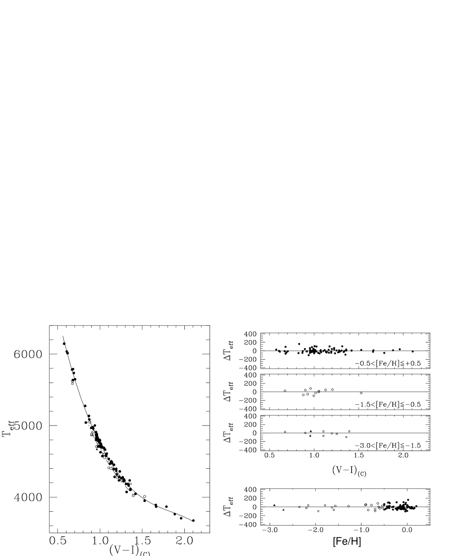
Figure 8: As in Fig. 2 for $T_{\mathrm{eff}}$ vs $(V-I)_{\mathrm{(C)}}$.

Even better is the calibration for $(V-I)_{\mathrm{(C)}}$ (Fig. 8):

$$\theta_{\mathrm{eff}} = 0.374+0.886(V-I)_{\mathrm{(C)}}$$ (8)

$$-0.197(V-I)_{\mathrm{(C)}}^{2}-0.008(V-I)_{\mathrm{(C)}}\mathrm{[Fe/H]}$$

which has $\sigma(T_{\mathrm{eff}})=46$ K and $N=111$. A residual correction is required here though (Table 1).

Eq. (8) is applicable in the following ranges:

$$+0.56<(V-I)_{\mathrm{(C)}}<+2.10 -0.5<\mathrm{[Fe/H]}<+0.5,$$ for

$$+0.85<(V-I)_{\mathrm{(C)}}<+1.20 -1.5<\mathrm{[Fe/H]}<-0.5,$$ for

$$+0.90<(V-I)_{\mathrm{(C)}}<+1.40 -2.5<\mathrm{[Fe/H]}<-1.5.$$ for

There is a steep $\Delta T_{\mathrm{eff}}/\Delta(V-I)_{\mathrm{(C)}}$ gradient from $(V-I)_{\mathrm{(C)}}=0.56$ to 1.30 for $\mathrm{[Fe/H]}=0$, which, later on decreases considerably to less than 10 K per 0.01 mag. The mean variation $\Delta T_{\mathrm{eff}}/\Delta\mathrm{[Fe/H]}$ is constant over the common ranges and amounts to approximately 10 K per 0.3 dex.

3.4 DDO system

There is a considerable number of stars with DDO photometry available in the GCPD though only in the range 3800 K$<T_{\mathrm{eff}}<$5800 K. Although DDO colors are severely affected by the star metallicity, the calibration formula obtained for the $C(42-48)$ color satisfactorily reproduces the effect and, surprisingly, its standard deviation is very close to the lowest to be found in this work.

Figure 9: As in Fig. 2 for $T_{\mathrm{eff}}$ vs $C(42-48)$.

For the $C(42-48)$ color index, we found:

$$\theta_{\mathrm{eff}} = 0.286+0.370[C(42-48)]-0.081\mathrm{[Fe/H]}$$ (9)

$$-0.009\mathrm{[Fe/H]}^{2}$$

with $\sigma(T_{\mathrm{eff}})=50$ K and $N=174$. Since the $\theta_{\mathrm{eff}}$ vs $C(42-48)$ relation is almost linear (for a given $\mathrm{[Fe/H]}$) the residuals of this original fit do not show any systematic tendency.

Figure 9 shows the sample and residuals of this last fit, whose ranges of applicability are:

$$+1.62<C(42-48)<+2.80 -0.5<\mathrm{[Fe/H]}<+0.5,$$ for

$$+1.70<C(42-48)<+2.64 -1.5<\mathrm{[Fe/H]}<-0.5,$$ for

$$+1.70<C(42-48)<+2.27 -2.5<\mathrm{[Fe/H]}<-1.5,$$ for

$$+1.68<C(42-48)<+1.80 -3.0<\mathrm{[Fe/H]}<-2.5.$$ for

As it is shown in Fig. 9, the $T_{\mathrm{eff}}$ vs $C(42-48)$ lines for constant $\mathrm{[Fe/H]}$ are almost parallel and thus the gradient $\Delta T_{\mathrm{eff}}/\Delta C(42-48)$ is nearly independent of $\mathrm{[Fe/H]}$. Their dependence on color is only slight, going from approximately 20 K per 0.01 mag at $C(42-48)=1.80$ to 10 K per 0.01 mag at $C(42-48)=2.70$. Due to the strong influence of $\mathrm{[Fe/H]}$ on this color index, the values of $\Delta T_{\mathrm{eff}}/\Delta\mathrm{[Fe/H]}$ for Eq. (9) are very high. At $C(42-48)=1.80$ the mean variation $\Delta T_{\mathrm{eff}}/\Delta\mathrm{[Fe/H]}$ amounts to 135 K per 0.3 dex for solar metallicity stars and gradually decreases to 60 K per 0.3 dex at $\mathrm{[Fe/H]}=-2$. At $C(42-48)=2.20$ these quantities reduce to 100 K per 0.3 dex and 50 K per 0.3 dex, respectively.

As stated previously, it is interesting to note the small values of the residuals of this fit, which are shown in the right panels of Fig. 9. They confirm that there are no systematic tendencies introduced by Eq. (9) with color or metallicity and that the large dispersion in the $T_{\mathrm{eff}}$ vs $C(42-48)$ relation can be attributed to well defined strong metallicity effects. They are also a consequence of an extremely careful photometric work.

Color ($X$)	Metallicity range	$P_{6}$	$P_{5}$	$P_{4}$	$P_{3}$	$P_{2}$	$P_{1}$	$P_{0}$	Eq.
$(V-S)$	$-0.5<\mathrm{[Fe/H]}<+0.5$		41913	$-139375$	173012	$-98788$	25624	$-2456.1$	2
$(V-S)$	$-1.5<\mathrm{[Fe/H]}<-0.5$			$-3693$	13603	$-18461$	11053	$-2410.6$	2
$(Y-V)$	$-0.5<\mathrm{[Fe/H]}<+0.5$	$-60268$	259060	$-442050$	379138	$-169791$	36864	$-2962.2$	3
$(Y-V)$	$-1.5<\mathrm{[Fe/H]}<-0.5$				2751.2	$-7813.5$	7405.1	$-2267.6$	3
$(Y-V)$	$-3.0<\mathrm{[Fe/H]}<-2.5$						294.14	$-129.34$	3
$(B_{2}-V_{1})$	$-0.5<\mathrm{[Fe/H]}<+0.5$	$-229.3$	1480.6	$-2382.8$	884.94	593.81	$-394.36$	$29.628$	4
$(B_{2}-V_{1})$	$-1.5<\mathrm{[Fe/H]}<-0.5$					$-604.77$	845.68	$-224.7$	4
$(B_{2}-G)$	$-0.5<\mathrm{[Fe/H]}<+0.5$			422.14	$-563.89$	$-88.665$	216.68	$-24.021$	5
$(B_{2}-G)$	$-1.5<\mathrm{[Fe/H]}<-0.5$				66.045	$-579.78$	515.79	$-30.683$	5
$t$	$-0.5<\mathrm{[Fe/H]}<+0.5$		3273.6	$-3220$	$-1575.9$	1879	$-127.21$	$-91.596$	6
$t$	$-1.5<\mathrm{[Fe/H]}<-0.5$			13196	$-21982$	11378	$-1776.3$	7.6382	6
$(V-I)_{\mathrm{(C)}}$	$-0.5<\mathrm{[Fe/H]}<+0.5$			497.01	$-2572.8$	4674.7	$-3470.1$	862.27	8
$(V-I)_{\mathrm{(C)}}$	$-3.0<\mathrm{[Fe/H]}<-0.5$						$-86.56$	104.53	8

Table 1: Polynomial fits to the original residuals. The general form is: $P=P_{6}X^{6}+\ldots+P_{2}X^{2}+P_{1}X+P_{0}$, where the $P_{i}$’s are constants and $X$ is the color. The last column specifies the equation that is being corrected.

3.5 Application to Arcturus

From the practical point of view, our calibrations allow one to obtain the effective temperature of a star from its color indices and atmospheric parameters $\log g$ (a distinction between dwarf and giant is enough) and $\mathrm{[Fe/H]}$. Arcturus (also HD 124897) is a well studied giant star, for which a recent direct effective temperature determination exists (Griffin & Lynas-Gray griffin99 (1999)). They derived $T_{\mathrm{eff}}=4290\pm 30$ K. Our calibration formulae provide the temperatures listed in Table 2. Their mean value is $4296\pm 28$ K, in excellent agreement with Griffin & Lynas-Gray result. It is worth remarking that this mean value is closer to the direct $T_{\mathrm{eff}}$ of Arcturus than the temperature derived through the IRFM: $4233\pm 55$ K (Alonso et al. 1999a ). This is a direct consequence of averaging stellar properties from large samples.

Color	Observed value	$T_{\mathrm{eff}}$ (K)
$(V-S)$	0.870	4253
$(Y-V)$	0.910	4281
$(B_{2}-V_{1})$	0.882	4312
$(B_{2}-G)$	0.764	4312
$t$	0.627	4297
$(R-I)_{\mathrm{(C)}}$	0.581	4346
$(V-I)_{\mathrm{(C)}}$	1.224	4296
$C(42-48)$	2.303	4271

Table 2: The effective temperature of Arcturus according to our calibrations. Different values have been derived through Eqs. (2)-(9) considering $\mathrm{[Fe/H]}=-0.54$ (Meléndez et al. melendez03j (2003)).

4 Comparison with other calibrations

4.1 Vilnius system

A good reference for this photometric system is Straižys (straizys95 (1995)) book. He has compiled several works on the intrinsic colors of stars of several spectral types in the Vilnius system and has smoothed them to build a single set of colors. This system is also described in Straižys & Sviderskiene (straizys72 (1972)).

Open circles in Fig. 10 show the intrinsic $(V-S)$ and $(Y-V)$ colors for giant stars according to Straižys ((straizys95, 1995, p. 440)), our calibrations for solar metallicity stars are also shown as solid lines. It is clear that for temperatures hotter than 5500 K, Straižys calibration predicts redder colors, the effect being larger for $(V-S)$. The difference can be as high as 400 K (6%) at $(V-S)\simeq 0.40$ or 500 K (6.7%) at $(Y-V)\simeq 0.30$ with no smooth tendencies. Below 5200 K the mean difference for $(Y-V)$ is about 1% and hardly exceeds 2%. The agreement for $(V-S)$ in this last range is remarkable.

The observed difference is partially explained by a gravity effect, as some of the hottest stars in Fig. 2 are supergiants. As a matter of fact, the lower a $\log g$ value is, a bluer $(V-S)$ is obtained (see Sect. 5.2).

Figure 10: Comparison of our calibrations for the Vilnius colors (solid lines) with those given by Straižys (straizys95 (1995)) (open circles).

4.2 Geneva system

Kobi & North (kobi90 (1990)) have published grids of $(B_{2}-V_{1})$ colors based on Kurucz models. A standard correction procedure was employed to put the synthetic colors into the observational system though only by using solar metallicity stars. Thus, as remarked by themselves, their results for metal-poor stars are only reliable if “Kurucz models correctly predict the differential effects of blanketing”. In Fig. 11 we compare our results for $\mathrm{[Fe/H]}=0$ (solid line) and $\mathrm{[Fe/H]}=-1$ (dashed line) with those of Kobi & North (filled circles correspond to the $\mathrm{[Fe/H]}=0$ grid while open circles correspond to the $\mathrm{[Fe/H]}=-1$ grid).

The slopes $\Delta T_{\mathrm{eff}}/\Delta(B_{2}-V_{1})$ are slightly different in Fig. 11, the sensitivity of $(B_{2}-V_{1})$ to the stellar effective temperature is slightly stronger in our calibration, which implies that Kobi & North colors result bluer in the high temperature range and redder below 6000 K. In the range 6000 K$<T_{\mathrm{eff}}<7000$ K there is good agreement.

It is also important to check the effect of $\mathrm{[Fe/H]}$ on $(B_{2}-V_{1})$ colors according to Kobi & North. Their colors are such that for a fixed $(B_{2}-V_{1})$, a change from $\mathrm{[Fe/H]}=0$ to $\mathrm{[Fe/H]}=-1$ reduces the effective temperature by about 170 K, independently of $(B_{2}-V_{1})$ in the range $0.25<(B_{2}-V_{1})<0.40$. Our calibration predicts a greater decrease, which amounts from 280 K to 190 K depending on the value of $(B_{2}-V_{1})$.

Figure 11: Comparison of our calibration for $\mathrm{[Fe/H]}=0$ (solid line) and $\mathrm{[Fe/H]}=-1$ (dotted line) with Kobi & North (kobi90 (1990)) $(B_{2}-V_{1})$ colors for $\mathrm{[Fe/H]}=0$ (filled circles) and $\mathrm{[Fe/H]}=-1$ (open circles).

4.3 $RI_{\mathrm{(C)}}$ system

Figures 12 and 13 show our calibrations for the $T_{\mathrm{eff}}$ vs $(R-I)_{\mathrm{(C)}}$ and $T_{\mathrm{eff}}$ vs $(V-I)_{\mathrm{(C)}}$ relations along with Bessell et al. (bessell98 (1998)) and Houdashelt et al. (houdashelt00 (2000)) results. The former of these provide colors obtained from ATLAS 9 overshoot models (squares) and no-overshoot models (triangles), which within our interval of interest differ by no more than 0.02 mag. Bessell et al. colors are valid for solar metallicity stars. On the other hand, Houdashelt et al. used improved MARCS models to calculate colors taking into account metallicity effects. Their results for $\mathrm{[Fe/H]}=0$ (filled circles) and $\mathrm{[Fe/H]}=-2$ (open circles) are shown. Both Bessell et al. and Houdashelt et al. provide colors for several $\log g$ values, Figs. 12 and 13 show their results for $\log g=2.0$, the nearest value to the peak of the $\log g$ distribution of the sample.

The $(R-I)_{\mathrm{(C)}}$ colors obtained from ATLAS 9 overshoot models agree slightly better than no-overshoot ones with ours below $T_{\mathrm{eff}}=5500$ K though Bessell et al. give too red colors in that range ($\sim 0.02$ mag). In the range 5750 K$<T_{\mathrm{eff}}<6250$ K, where no-overshoot models seem to be more reliable (see also Castelli et al. castelli97 (1997)) the agreement increases with temperature. In the case of the $(V-I)_{\mathrm{(C)}}$ color, below $T_{\mathrm{eff}}=5500$ K there is an almost constant difference of about 0.04 mag that makes our colors (for $\mathrm{[Fe/H]}=0$ stars) slightly bluer compared to both overshoot and no-overshoot model colors (only no-overshoot results are plotted).

Houdashelt et al. $(R-I)_{\mathrm{(C)}}$ colors are too blue for $T_{\mathrm{eff}}>5500$ K. The effect gradually increases as hotter stars are considered. At $T_{\mathrm{eff}}=5500$ K, for instance, the difference amounts to 0.015 mag while at $T_{\mathrm{eff}}=6250$ K it is about 0.050 mag. A similar behaviour was also present in the dwarf calibration (see our Fig. 12c in Paper I). Below $T_{\mathrm{eff}}=5000$ K, there is good agreement since both the gradient $\Delta T_{\mathrm{eff}}/\Delta(R-I)_{\mathrm{(C)}}$ and $(R-I)_{\mathrm{(C)}}$ colors are very similar. Even though Houdashelt et al. colors were put into the observational system by means of a sample of solar metallicity stars and thus their results for metal-poor stars could be not very accurate, the fact that metal-poor stars are redder than solar metallicity stars for the $(R-I)_{\mathrm{(C)}}$ color index is very well reproduced and agrees reasonably well with our result. Nevertheless, according to our calibration, for a fixed temperature, the difference in $(R-I)_{\mathrm{(C)}}$ between a solar metallicity star and a $\mathrm{[Fe/H]}=-1$ star is no more than 0.02 mag while Houdashelt et al. give 0.04 mag. On the other hand, their $(V-I)_{\mathrm{(C)}}$ colors for solar metallicity stars are very close to ours, except at high temperatures.

Figure 12: Comparison of our calibration for $(R-I)_{\mathrm{(C)}}$ for $\mathrm{[Fe/H]}=0$ (solid lines) and $\mathrm{[Fe/H]}=-2$ (dashed line) with the $(R-I)_{\mathrm{(C)}}$ colors obtained by: Bessell et al. (bessell98 (1998)) from ATLAS 9 overshoot models (squares) and ATLAS 9 no-overshoot models (triangles), Houdashelt et al. (houdashelt00 (2000)) for $\mathrm{[Fe/H]}=0$ (filled circles) and $\mathrm{[Fe/H]}=-2$ (open circles).

Figure 13: As in Fig. 12 for $(V-I)_{\mathrm{(C)}}$.

4.4 DDO system

Filled and open circles in Fig. 14 correspond to DDO colors for $\mathrm{[Fe/H]}=0$ and $\mathrm{[Fe/H]}=-1$ derived from synthetic MARCS spectra by Tripicco & Bell (tripicco91 (1991)). Their procedure to put the synthetic colors into the observational system involves the use of spectrophotometric scans, a procedure that allows a model independent treatment. For stars having $T_{\mathrm{eff}}>4500$ K, Tripicco & Bell colors are too red but the effect of $\mathrm{[Fe/H]}$ is well reproduced. Particularly, in the range 4500 K$<T_{\mathrm{eff}}<5000$ K, $C(42-48)$ varies 0.15 mag for a 1.0 dex variation in $\mathrm{[Fe/H]}$, in reasonable agreement with the mean 0.12 mag variation that Eq. (9) produces. Contrary to our calibration, in which $T_{\mathrm{eff}}$ vs $C(42-48)$ lines of constant $\mathrm{[Fe/H]}$ are almost parallel, Tripicco & Bell results suggest stronger metallicity effects for stars hotter than 5000 K and cooler than 4500 K. In general, the slopes $\Delta T_{\mathrm{eff}}/\Delta C(42-48)$ are quite different, specially for $\mathrm{[Fe/H]}=-1$.

The empirical calibration of Clariá et al. (claria94 (1994)) for the $T_{\mathrm{eff}}$ vs $C(42-48)$ relation is shown in Fig. 14 with open triangles. They used the $C(42-45):C(45-48)$ color-color diagram to derive mean DDO colors for different spectral types, for which a $T_{\mathrm{eff}}$ calibration was also derived. The agreement with our work is quite good, specially for $T_{\mathrm{eff}}<4600$ K. In the range 4600 K$<T_{\mathrm{eff}}<5000$ K there is a shift of only 0.04 mag that makes Clariá et al. colors slightly bluer than ours.

Finally, Morossi et al. (morossi95 (1995)) have used Kurucz models to derive synthetic DDO colors for solar metallicity stars as a function of spectral type. The mean DDO effective temperature-MK spectral type provided by Clariá et al. (claria94 (1994)) was adopted here to derive the $T_{\mathrm{eff}}$ vs $C(42-48)$ relation corresponding to Morossi et al. colors. This relation provides too red colors in the range 4100 K$<T_{\mathrm{eff}}<4600$ K but agrees with our color for $T_{\mathrm{eff}}=3950$ K. The slope $\Delta T_{\mathrm{eff}}/\Delta C(42-48)$ changes dramatically with color, so that around $T_{\mathrm{eff}}=4700$ K the agreement is good again but for hotter stars Morossi et al. colors become slightly bluer.

Figure 14: Comparison of our calibration for $C(42-48)$ for $\mathrm{[Fe/H]}=0$ (solid line) and $\mathrm{[Fe/H]}=-1$ (dashed line) with: Tripicco & Bell (tripicco91 (1991)) calibrations for $\mathrm{[Fe/H]}=0$ (filled circles) and $\mathrm{[Fe/H]}=-1$ (open circles), Clariá et al. (claria94 (1994)) colors (triangles), and Morossi et al. (morossi95 (1995)) colors (squares).

5 The effective temperature scale

5.1 Intrinsic colors of giant stars

Instead of fitting the $\mathrm{color}=\mathrm{color}(T_{\mathrm{eff}},\mathrm{[Fe/H]})$ relation to some analytical function from the same sample adopted to derive the $T_{\mathrm{eff}}=T_{\mathrm{eff}}(\mathrm{color},\mathrm{[Fe/H]})$ relation, as is sometimes done, we solved Eqs. (2)-(9) for the color index as a function of $T_{\mathrm{eff}}$ and $\mathrm{[Fe/H]}$ in order to derive the intrinsic colors of giant stars. The former procedure does not guarantee a single correspondence between the three quantities involved and could produce a temperature scale inconsistent with the calibration formulae.

Tables 3, 4 and 5 list the intrinsic colors of giant stars as a function of $T_{\mathrm{eff}}$ and $\mathrm{[Fe/H]}$, including some reliable extrapolated values. They have been used to plot the color-color diagrams of Figs. 15 and 16, in which we also show the derreddened colors of some giant stars with $\mathrm{[Fe/H]}>-0.5$. These stars have been introduced to verify that our calibrations satisfactorily reproduce the empirical color-color diagrams. We attribute the observed dispersion to the amplitude of the $\mathrm{[Fe/H]}$ interval covered and to the fact that only a few stars have $\mathrm{[Fe/H]}>0$.

	$(V-S)$			$(Y-V)$
$T_{\mathrm{eff}}$	$\mathrm{[Fe/H]}=0.0$	$-1.0$	$-2.0$	$\mathrm{[Fe/H]}=0.0$	$-1.0$	$-2.0$
3750	1.109	-	-	-	-	-
3800	1.095	-	-	1.152	-	-
4000	1.008	0.935	0.952	1.059	0.969	-
4250	0.880	0.853	0.864	0.961	0.870	0.886
4500	0.798	0.779	0.785	0.866	0.787	0.796
4750	0.735	0.712	0.715	0.782	0.717	0.718
5000	0.682	0.653	0.652	0.713	0.657	0.648
5250	0.633	0.600	0.594	0.654	0.606	0.587
5500	0.586	0.553	-	0.602	0.560	-
5750	0.541	0.511	-	0.554	0.520	-
6000	0.497	-	-	0.509	-	-
6250	0.454	-	-	0.466	-	-
6500	0.413	-	-	0.425	-	-
6750	0.374	-	-	0.386	-	-
7000	0.338	-	-	0.350	-	-
7250	0.307	-	-	0.317	-	-
7500	0.278	-	-	0.287	-	-
7750	0.253	-	-	0.261	-	-

Table 3: Intrinsic colors of giant stars in the Vilnius system as a function of $\mathrm{[Fe/H]}$.

	$(B_{2}-V_{1})$			$(B_{2}-G)$			$t$
$T_{\mathrm{eff}}$	$\mathrm{[Fe/H]}=0.0$	$-1.0$	$-2.0$	$\mathrm{[Fe/H]}=0.0$	$-1.0$	$-2.0$	$\mathrm{[Fe/H]}=0.0$	$-1.0$	$-2.0$
3500	-	-	-	-	-	-	0.990	-	-
3750	1.224	-	-	1.198	-	-	0.909	-	-
4000	1.077	1.052	-	1.028	0.984	-	0.790	0.776	-
4250	0.931	0.870	0.871	0.838	0.731	0.726	0.646	0.660	0.654
4500	0.803	0.733	0.729	0.658	0.549	0.546	0.526	0.524	0.542
4750	0.693	0.623	0.604	0.503	0.403	0.385	0.430	0.420	0.442
5000	0.599	0.528	0.494	0.371	0.279	0.240	0.348	0.339	0.353
5250	0.515	0.446	0.396	0.257	0.172	0.109	0.276	0.270	0.271
5500	0.440	0.373	0.308	0.155	0.076	$-0.010$	0.209	0.208	0.197
5750	0.371	0.307	-	0.064	$-0.010$	-	0.147	0.147	-
6000	0.307	0.248	-	$-0.020$	$-0.089$	-	0.088	0.085	-
6250	0.249	-	-	$-0.097$	-	-	0.031	-	-
6500	0.194	-	-	$-0.170$	-	-	$-0.023$	-	-
6750	0.144	-	-	$-0.239$	-	-	$-0.076$	-	-
7000	0.097	-	-	$-0.303$	-	-	$-0.126$	-	-
7250	0.053	-	-	$-0.365$	-	-	$-0.173$	-	-
7500	0.013	-	-	$-0.425$	-	-	$-0.218$	-	-
7750	$-0.025$	-	-	$-0.481$	-	-	$-0.260$	-	-
8000	$-0.060$	-	-	$-0.536$	-	-	$-0.299$	-	-
8250	$-0.093$	-	-	$-0.588$	-	-	-	-	-

Table 4: As in Table 3 for the Geneva system.

	$(R-I)_{\mathrm{(C)}}$			$(V-I)_{\mathrm{(C)}}$			$C(42-48)$
$T_{\mathrm{eff}}$	$\mathrm{[Fe/H]}=0.0$	$-1.0$	$-2.0$	$\mathrm{[Fe/H]}=0.0$	$-1.0$	$-2.0$	$\mathrm{[Fe/H]}=0.0$	$-1.0$	$-2.0$
3750	-	-	-	1.941	-	-	2.859	-	-
4000	0.699	-	0.718	1.491	-	-	2.632	2.438	-
4250	0.605	0.611	0.618	1.269	-	1.233	2.432	2.238	2.092
4500	0.534	0.539	0.544	1.118	1.097	1.078	2.254	2.059	1.914
4750	0.478	0.482	0.486	1.000	0.971	0.956	2.095	1.900	1.754
5000	0.431	0.434	0.438	0.902	0.869	-	1.951	1.757	-
5250	0.392	0.395	0.397	0.817	-	-	1.822	-	-
5500	0.358	0.360	0.363	0.742	-	-	1.704	-	-
5750	0.328	0.330	0.332	0.675	-	-	1.596	-	-
6000	0.302	0.304	0.306	0.615	-	-	-	-	-
6250	0.278	0.280	0.282	0.561	-	-	-	-	-

Table 5: As in Table 3 for the $RI_{\mathrm{(C)}}$ and DDO systems.

Figure 15: $(R-I)_{\mathrm{(C)}}$ vs $(Y-V)$, color-color diagram showing lines of equal $T_{\mathrm{eff}}$ and $\mathrm{[Fe/H]}$. Crosses correspond to derreddened colors of some giant stars with $\mathrm{[Fe/H]}>-0.5$.

Figure 16: As in Fig. 15 for $t$ vs $C(42-48)$.

5.2 Gravity effects

Colors derived in this work for giants generally differ from those given for main sequence stars in Paper I. Even though the mean differences are of the order of the observational errors, so that they are not very useful when studying individual stars, knowledge of gravity effects on the empirical temperature scale may improve our understanding of stellar spectra. The difference in color between a giant and a dwarf star of the same $T_{\mathrm{eff}}$ is plotted in Fig. 17 for stars with $\mathrm{[Fe/H]}=0$. Different symbols and line styles correspond to different color indices.

Firstly, it is worth noticing that $(R-I)_{\mathrm{(C)}}$ is almost unaffected by the surface gravity, dwarfs are only 0.03 mag redder than giants at $T_{\mathrm{eff}}=4000$ K and non-distinguishable from them at high temperatures. Given that it is also nearly independent of $\mathrm{[Fe/H]}$, this color is a good $T_{\mathrm{eff}}$ indicator, free of secondary effects.

For most colors, main sequence F stars are redder than F giants. The difference seems to increase with the separation between the wavelength bands covered by each filter. It is large (0.07 mag at $T_{\mathrm{eff}}=7000$ K) for $(B_{2}-G)$, whose $B_{2}$ filter has a mean wavelength that is about 1300Å away from the $G$ one. It is relatively large (0.06 mag) for $(V-S)$, for which the separation is approximately 1100Å, and less prominent (0.04 mag) for $(Y-V)$ and $(B_{2}-V_{1})$, whose separations are around 850Å. Neutral hydrogen bound-free opacity increases more with wavelength than that of the H^- ion, which is the only of the two that increases with electron pressure, and so is stronger in main sequence stars. This implies that the wavelength dependence of the total opacity is smoother for dwarfs and stronger for giants. As a result, within Paschen continuum (365–830 nm), giants gradually emit more radiation at shorter wavelengths than dwarfs, an effect that is well reproduced in Kurucz SEDs. Therefore, in addition to their primary dependence on $T_{\mathrm{eff}}$, colors at well separated wavelength intervals within Paschen continuum will be more affected by the surface gravity. Alonso et al. (1999b ) also showed this effect for $(B-V)$ and $(V-I)$ and provided a similar explanation.

On the other hand, UV and optical colors of K stars are affected by different mechanisms, which can make a giant bluer or redder than a main sequence star. In addition to their dependence with the continuum opacity, at the low $T_{\mathrm{eff}}$s found in K stars, stellar spectra are crowded with lots of lines that can be stronger in giants (e.g. CH lines) or in dwarfs (e.g. MgH lines), as explained by Tripicco & Bell (tripicco91 (1991)) and Paltoglou & Bell (paltoglou94 (1994)).

Though it is not shown here, we have also checked that colors for metal-poor stars are only slightly affected by the surface gravity.

Figure 17: Gravity effects on photometric color indices. The vertical axis measures the difference in color between a solar metallicity giant and a main sequence star as a function of $T_{\mathrm{eff}}$. A giant is redder than a main sequence star of the same effective temperature when $\Delta$(color) is positive. Colors plotted are: $(V-S)$ (dotted line), $(Y-V)$ (open circles), $(B_{2}-V_{1})$ (dashed line), $(B_{2}-G)$ (long-dashed line), $(R-I)_{\mathrm{(C)}}$ (filled circles), $(V-I)_{\mathrm{(C)}}$ (triangles), and $C(42-48)$ (dash-dotted line).

5.3 Giants in clusters

The effective temperature scale derived in this work reproduces well the $T_{\mathrm{eff}}$ versus color relations of open and old globular clusters, as is shown in Fig. 18 for the $C(42-48)$ color. Table 6 contains the temperatures of the stars in this figure as given by Alonso et al. (1999b ) and intrinsic colors from the GCPD corrected by using the $E(B-V)$ values given by KI03. The observed deviations are within the observational errors, which can be verified from the error bars to the upper right corner of Fig. 18. From this result not only we conclude that the temperature scale derived here is suited for stars in clusters, but also we are showing that the metallicity and reddening scales for these clusters (KI03) are well determined.

Star	$T_{\mathrm{eff}}$	$C(42-48)$	Star	$T_{\mathrm{eff}}$	$C(42-48)$	Star	$T_{\mathrm{eff}}$	$C(42-48)$
M3 III28	4073	2.261	M67 231	4869	2.035	47Tuc 4418	3940	2.557
M3 IV25	4324	2.087	M67 244	5086	1.914	47Tuc 5406	4181	2.310
M3 216	4490	1.956	M67 I17	4933	1.996	47Tuc 5427	4229	2.298
M67 84	4748	2.102	M67 IV20	4627	2.093	47Tuc 5527	4494	2.043
M67 105	4452	2.301	M92 III13	4123	2.206	47Tuc 5529	3792	2.648
M67 108	4222	2.439	M92 VII18	4207	2.105	47Tuc 5627	4174	2.308
M67 141	4755	2.091	M92 XII8	4425	1.893	47Tuc 5739	4062	2.449
M67 151	4802	2.091	M92 IV10	4553	1.830	47Tuc 6509	4498	2.144
M67 164	4698	2.119	M92 IV2	4602	1.796	NGC362 I44	4289	2.195
M67 170	4264	2.398	M92 IV114	4652	1.739	NGC362 II43	4610	1.969
M67 223	4717	2.106	M92 III4	4992	1.633	NGC362 II47	4731	1.819
M67 224	4703	2.104	47Tuc 3407	4280	2.266	NGC362 III4	4307	2.149

Table 6: Temperatures and (intrinsic) colors for the stars plotted in Fig. 18.

Figure 18: $T_{\mathrm{eff}}$ vs $C(42-48)$ relations for giants in the open cluster M67 (filled circles) and in the globular clusters 47 Tuc (open circles), NGC 362 and M3 (filled squares), and M92 (open squares). Solid, dotted, dashed and long-dashed lines correspond to our calibrations for $\mathrm{[Fe/H]}=-0.08$, $\mathrm{[Fe/H]}=-0.70$, $\mathrm{[Fe/H]}=-1.50$ and $\mathrm{[Fe/H]}=-2.38$, respectively, which are the mean metallicities of the clusters. Error bars are shown to the upper right corner of this figure.

5.4 Evolutionary calculations

One of the most important applications of the temperature scale is the transformation of theoretical HR diagrams into CMDs since it allows to explore the capability of evolutionary calculations to reproduce the observations.

Here we compare isochrones with fiducial lines for two globular clusters: NGC 6553 and M3. Figure 19 shows these fiducial lines along with theoretical isochrones for $\mathrm{[Fe/H]}=-0.2$, ($[\alpha/\mathrm{Fe}]=+0.2$) and $\mathrm{[Fe/H]}=-1.5$ ($[\alpha/\mathrm{Fe}]=+0.3$) and ages $t=11,$ 13 and 15 Gyr; according to Yi et al. (yi03 (2003), Y²). Also shown is the Bergbusch & VandenBerg (bergbusch01 (2001), BV01) isochrone for $\mathrm{[Fe/H]}=-1.5$ ($[\alpha/\mathrm{Fe}]=+0.3$) and $t=13$ Gyr.

The bulge globular cluster NGC 6553 serves as a template for metal-rich galactic populations (ellipticals and bulges) given that it is one of the most metal-rich globular clusters of the Galaxy ($\mathrm{[Fe/H]}=-0.2$, Melendez et al. melendez03j (2003)). Data for this cluster are from Guarnieri et al. (guarnieri98 (1998)) and Ortolani et al. (ortolani95 (1995)). Their HST $(V-I)_{\mathrm{(C)}}$ colors have been transformed into $T_{\mathrm{eff}}$ by using our calibrations for both dwarfs (Paper I) and giants. We adopted $E(V-I)$ and $(m-M)$ from Guarnieri et al. (1998). The best fit occurs at $t=13$ Gyr, in agreement with the old age obtained by Ortolani et al. (ortolani95 (1995)).

For the halo globular cluster M3 ($\mathrm{[Fe/H]}=-1.5$, KI03), almost all the photometry is from HST (Rood et al. rood99 (1999)), the last three points on the main sequence are ground-base observations (Johnson & Bolte johnson98 (1998)) corrected for blending using the HST data. The $E(B-V)$ and $(m-M)$ values were also taken from KI03. Again, colors were transformed into $T_{\mathrm{eff}}$ from our temperature scale. In order to obtain a reasonable agreement with the models, M3 photometry has been empirically corrected by $\Delta T_{\mathrm{eff}}=+60$ K and $\Delta(m-M)=+0.2$ to fit the turnoff of the Y² isochrones. Likewise, the BV01 isochrone has been shifted to fit the observed turnoff.

Note that only a small adjustment is required to obtain a better fit to the data, the $\Delta T_{\mathrm{eff}}=+60$ K is equivalent to a correction of only 0.014 mag in $(V-I)_{\mathrm{(C)}}$ (or $\Delta E(B-V)=0.01$ mag), and the correction for the absolute magnitude is well between the error bars for the distance modulus. For M3, $(m-M)$ ranges from 14.8 (Kraft et al. kraft92 (1992)) to 15.2 (BV01). A correction of 0.2 mag in $M_{V}$ corresponds to a change of only 0.02 dex in the iron abundance obtained from Fe II (KI03). It is important to note that the isochrone of BV01 satisfactorily reproduces the observed RGB, but the Y² isochrones fit better the low main sequence.

Figure 19: Left: Fiducial line for NGC 6553 according to Guarnieri et al. (guarnieri98 (1998)) and Ortolani et al. (ortolani95 (1995)) transformed to the $M_{V}$ vs $T_{\mathrm{eff}}$ plane from our calibrations (open circles). The solid lines are theoretical isochrones calculated by Yi et al. (yi03 (2003)). Right: As in the left panel for M3 (Root et al. rood99 (1999), Johnson & Bolte johnson98 (1998)). The dotted line is an isochrone from Bergbusch & VandenBerg (bergbusch01 (2001), BV01) grids.

6 Conclusions

We have calibrated the effective temperature versus color relations for several color indices in 4 important photometric systems using reliable and recent $\mathrm{[Fe/H]}$ and $\log g$ measurements to explore with improved accuracy the effects of chemical composition and surface gravity on the temperature scale.

In general, the present calibrations span the following ranges: 3800 K$<T_{\mathrm{eff}}<$8000 K, $-3.0<\mathrm{[Fe/H]}<+0.5$. Ranges of applicability, however, are different and specific for each color calibration. For $(R-I)_{\mathrm{(C)}}$ and $C(42-48)$, for example, these ranges are not so wide, specially in $T_{\mathrm{eff}}$. We also provide specific ranges of applicability after every formula.

The standard deviation of the fits amount from 46 K for $(V-I)_{\mathrm{(C)}}$ to 99 K for $(Y-V)$ with more than 130 stars in almost every calibration. Residuals of every fit were iteratively checked to reduce the dispersion and undesirable systematic effects.

Finally, from our formulae we have calculated the intrinsic colors of giant stars and have probed their consistency with empirical color-color diagrams, gravity effects on stellar spectra, $T_{\mathrm{eff}}$ versus color relations for stars in clusters and evolutionary calculations. Our results for the main sequence were also explored in this last case.

- (1) Alonso, A., Arribas, S., & Martínez-Roger, C. 1996a, A&AS, 117, 227
- (2) Alonso, A., Arribas, S., & Martínez-Roger, C. 1996b, A&A, 313, 873
- (3) Alonso, A., Arribas, S., & Martínez-Roger, C. 1999a, A&AS, 139, 335
- (4) Alonso, A., Arribas, S., & Martínez-Roger, C. 1999b, A&AS, 140, 261
- (5) Bell R. A. 1997, Tests of effective temperature–color relations. In Proceedings of IAU Symp. 189, “Fundamental Stellar Properties: the interaction between observation and theory”, ed. T. R. Bedding, A. J. Booth, & J. Davis. Kluwer Academic Publishers, 159
- (6) Bergbusch, P. A., & VandenBerg, D. A. 2001, ApJ, 556, 322 (BV01)
- (7) Bessell, M. S. 1979, PASP, 91, 589
- (8) Bessell, M. S., Castelli, F., & Plez, B. 1998, A&A, 333, 231
- (9) Bessell, M. S. 2001, PASP, 113, 66
- (10) Castelli, F., Gratton, R. G., & Kurucz, R. L. 1997, A&A, 318, 841
- (11) Cayrel de Strobel, G., Hauck, B., François, T., et al. 1992, A&AS, 95, 273
- (12) Cayrel de Strobel, G., Soubiran, C., & Ralite, N. 2001, A&A, 373, 159
- (13) Clariá, J. J., Piatti, A. E., & Lapasset, E. 1994, PASP, 106, 436
- (14) Cramer, N. 1999, NewAr, 43, 343
- (15) Girardi, L., Bertelli, G., Bressan, A., et al. 2002, A&A, 391, 195
- (16) Griffin, R. E. M., & Lynas-Gray, A. E. 1999, AJ, 117, 2998
- (17) Guarnieri, M. D., Ortolani, S., Montegriffo, P., et al. 1998, A&A, 331, 70
- (18) Hauck, B. & Künzli, M. 1996, Baltic Astron., 5, 303
- (19) Heiter, U., & Luck, R. E. 2003, Abundance analysis of planetary host stars. In proceedings of IAU Symp. 210, “Modelling of Stellar Atmospheres”, ed. N. Piskunov, W.W. Weiss, & D.F. Gray, ASP Conference Series, in press
- (20) Hilker, M. 2000, A&A, 355, 994 (H00)
- (21) Houdashelt, M. L., Bell, R. A, & Sweigart, A. V. 2000, AJ, 119, 1448
- (22) Johnson, J. A., Bolte, M. 1998, AJ, 115, 693
- (23) Kobi, D., & North, P. 1990, A&AS, 85, 999
- (24) Kraft, R., Sneden, C., Langer, G. E., & Prosser, C. 1992, AJ, 104, 645
- (25) Kraft, R., & Ivans, I. 2003, PASP, 115, 143 (KI03)
- (26) Ortolani, S., Renzini, A., Gilmozzi, R., et al. 1995, Nature, 377, 701
- (27) Meléndez, J., & Barbuy, B. 2002, ApJ, 575, 474
- (28) Melendez, J., Barbuy, B., Bica, B., et al. 2003, A&A, 411, 417
- (29) Meléndez, J., & Ramírez, I. 2003, A&A, 398, 705 (Paper I)
- (30) Mermilliod, J. C., Mermilliod, M., & Hauck, B. 1997, A&AS, 124, 349 (GCPD)
- (31) Mishenina, T. V., & Kovtyukh V. V. 2001, A&A, 370, 951
- (32) Morossi, C., Franchini, M., Malagnini, M. L., & Kurucz, R. L. 1995, A&A, 295, 471
- (33) Nissen, P. E., Primas, F., Asplund, M., & Lambert, D. L. 2002, A&A, 390, 235
- (34) Paltoglou, G., & Bell, R. A. 1994, MNRAS, 268, 793
- (35) Rood, R. T., Carretta, E., Paltrinieri, B., et al. 1999, ApJ, 523, 752
- (36) Ryan, S. G., Norris, J. E., & Beers, T. C. 1999, ApJ, 523, 654
- (37) Santos, N. C., Israelian, G. & Mayor, M. 2001, A&A, 373, 1019
- (38) Smith, V., Hinkle, K. H., Cunha, K., et al. 2002, AJ, 124, 3241
- (39) Stephens, A., & Boesgaard, A. M. 2002, AJ, 123, 1647
- (40) Straižys, V., & Sviderskiene, Z. 1972, A&A, 17, 312
- (41) Straižys, V. 1995, in Multicolor Stellar Photometry (Pachart Publishing House), 430
- (42) Takada-Hiday, M., Takeda, Y., Sato, S., et al. 2002, ApJ, 573, 614
- (43) Tripicco, M., & Bell, R. A. 1991, AJ, 102, 744
- (44) Yi, S. K., Kim, Y., & Demarque, P. 2003, ApJS, 144, 259 (Y2)
- (45) Yong, D., & Lambert, D. L. 2003, PASP, 115, 22