EMPIRICALLY CONSTRAINED COLOR-TEMPERATURE
RELATIONS. II. $uvby^{1,\,2}$

Abstract

A new grid of theoretical color indices for the Strömgren $uvby$ photometric system has been derived from MARCS model atmospheres and SSG synthetic spectra for cool dwarf and giant stars having $-3.0\leq\rm{[Fe/H]}\leq+0.5$ and $3000\leq T_{\rm{eff}}\leq 8000\,$K. At warmer temperatures (i.e., $8000<T_{\rm{eff}}\leq 40000\,$K), this grid has been supplemented with the synthetic $uvby$ colors from recent Kurucz atmospheric models without overshooting (Castelli, Gratton, & Kurucz, 1997, A&A, 318, 841). Our transformations appear to reproduce the observed colors of extremely metal-poor turnoff and giant stars: the various $uvby$ color-magnitude diagrams (CMDs) for the $\rm{[Fe/H]}\sim-2.2$ globular cluster M 92 can be matched exceedingly well down to $M_{V}\approx 6$ by the same isochrone that provides a very good fit to published $BV$ data (see Paper I), on the assumption of the same distance and reddening. Due to a number of assumptions made in the synthetic color calculations, however, our color–$T_{\rm eff}$ relations for cool stars fail to provide a suitable match to the $uvby$ photometry of both cluster and field stars having $\rm{[Fe/H]}>-2.0$. To overcome this problem, the theoretical indices at intermediate and high metallicities have been corrected using a set of color calibrations based on field stars having well-determined distances from Hipparcos, accurate $T_{\rm{eff}}$ estimates from the infrared flux method, and spectroscopic $\rm{[Fe/H]}$ values. In contrast with Paper I, star clusters played only a minor role in this analysis in that they provided a supplementary constraint on the color corrections for cool dwarf stars with $T_{\rm{eff}}\leq 5500\,$K. They were mainly used to test the color–$T_{\rm eff}$ relations and, encouragingly, isochrones that employ the transformations derived in this study are able to reproduce the observed CMDs (involving $u-v$, $v-b$, and $b-y$ colors) for a number of open and globular clusters (including M 67, the Hyades, and 47 Tuc) rather well. Moreover, our interpretations of such data are very similar, if not identical, with those given in Paper I from a consideration of $BV(RI)_{C}$ observations for the same clusters — which provides a compelling argument in support of the color–$T_{\rm eff}$ relations that are reported in both studies. In the present investigation, we have also analyzed the observed Strömgren photometry for the classic Population II subdwarfs, compared our “final” $(b-y)$–$T_{\rm{eff}}$ relationship with those derived empirically in a number of recent studies, and examined in some detail the dependence of the $m_{1}$ index on $\rm{[Fe/H]}$.

1 Introduction

Among the wide variety of photometric systems available today, the $uvby$ system of Strömgren (1963) still remains one of the most valuable for the study of stellar populations and Galactic structure. Its usefulness stems from the fact that the four intermediate-width filters are designed to isolate and measure certain key features in a stellar spectrum which are highly sensitive to the underlying physical characteristics of the star itself. For example, Strömgren $b-y$ provides an accurate indicator of effective temperature similar to broadband $B-V$ or $V-I$ while the two other Strömgren indices, $m_{1}$ and $c_{1}$, yield photometric estimates of the stellar metal abundance and surface gravity (or luminosity). In this respect, the ability of the $uvby$ system to provide precise estimates of these fundamental parameters makes it much better suited than standard Johnson-Cousins $UBVRI$ photometry for the study of individual stars.

For years, Strömgren photometry has provided a wealth of information on the chemical and dynamical evolution of the Milky Way through its application to the field-star populations in both the Galactic halo and the solar neighborhood (see, for example, the works of Clegg & Bell, 1973; Schuster & Nissen, 1988, 1989a, 1989b; Olsen, 1984; Haywood, 2001). Moreover, it has also proven to be extremely valuable in its application to star clusters. While the narrowness of the $uvby$ filters limited earlier investigations (Crawford & Barnes, 1969, 1970a; Crawford & Perry, 1966, 1976) primarily to those stars in nearby open clusters (e.g., the Hyades, NGC 752, Praesepe, and the Pleiades) that were bright and isolated enough to be readily observed using traditional photomultipliers, the advent of modern CCD detectors meant that the Strömgren system could be extended to much fainter stars such as those found near the turnoff and main sequence regions in more distant clusters (see the pioneering studies of Anthony-Twarog, 1987a, b; Anthony-Twarog & Twarog, 1987). This recent explosion in the amount of high-quality Strömgren data for a large number of open and globular clusters offers profound potential for refining our understanding of these systems. For instance, it has already been shown that both the $m_{1}$ and $c_{1}$ indices can reveal the existence of carbon and nitrogen abundance variations in globular cluster RGB stars (Hilker, 2000; Grundahl et al., 2002a). Moreover, the $c_{1}$ index has also been used to derive distance-independent cluster ages using techniques akin to those developed by Schuster & Nissen (1989b) for field stars (Grundahl et al., 2000a) while the $m_{1}$ index has provided photometric $\rm{[Fe/H]}$ estimates for individual turnoff and giant stars (Nissen, Twarog, & Crawford, 1987; Hughes & Wallerstein, 2000; Hilker & Richtler, 2000).

Despite the availability of new high-quality $uvby$ photometry for a number of open and globular clusters in the Galaxy, our ability to fully exploit these data using stellar evolutionary models still remains somewhat difficult due to the lack of accurate and reliable color–$T_{\rm{eff}}$ relations and bolometric corrections for the Strömgren system that are needed to transform these theoretical models to the observed cluster color-magnitude diagrams (CMDs). While a number of empirical calibrations and analytical formulae have been derived over the years that serve to relate the Strömgren $b-y$, $m_{1}$, and $c_{1}$ indices to the fundamental stellar parameters of $T_{\rm{eff}}$, $\rm{[Fe/H]}$, and $\rm{log~{}g}$, respectively, they are often very specific to certain types of stars that occupy limited regions of the H-R diagram and generally rely on only a small number of stars in the solar neighborhood that have well-determined properties from spectroscopic analysis. As a result, these relations cannot be trusted if they are applied to situations beyond the range in which they were originally intended. Alternatively, one may employ grids of theoretical colors computed from model stellar atmospheres and synthetic spectra to interpret the photometric data (Bell, 1988). These synthetic colors are very useful for not only confirming the empirical calibrations between various Strömgren indices and certain stellar properties, but also for characterizing the nature of stars in those regimes not covered by these relations. Furthermore, they are ideal for transforming evolutionary models to the observational color-magnitude and color-color planes owing to their broad coverage of stellar parameter space. Their accuracy, however, is ultimately limited by how well the models are able to reproduce the observed spectrum of an actual star. Some examples of these synthetic color computations for the $uvby$ system include the grid of MARCS colors for cool dwarfs and subgiants presented by VandenBerg & Bell (1985) and those computed by Kurucz from his atmospheric models (Kurucz, 1993). While the $uvby$ colors of the latter cover a much larger range in stellar parameter space than the VandenBerg & Bell results, they are known to have problems reproducing the observed colors of cooler dwarf and giant stars (Grundahl, VandenBerg, & Andersen, 1998). Therefore, in order to accurately interpret and analyze cluster $uvby$ photometry using current stellar models, we must first check if these theoretical colors are in good agreement with the observed photometry for a collection of stars with well-determined physical properties.

Recently, VandenBerg & Clem (2003, hereafter Paper I) found that, by applying small corrections to synthetic color transformations for the $BV(RI)_{C}$ system towards cooler effective temperatures, it is possible to achieve good consistency with the observational data for cool dwarf and giant stars in both the metal-poor and metal-rich regimes. Their so-called “semi-empirical” approach resulted in a set of $BV(RI)_{C}$ color–$T_{\rm{eff}}$ relations and bolometric corrections that were able to accurately and consistently interpret the observed $B-V$, $V-I$, and $V-R$ CMDs for both a sample of clusters (such as the Hyades, M 67, M 92, 47 Tuc, and NGC 6791) and Hipparcos field stars. In addition, their predicted solar metallicity $(B-V)$–$T_{\rm{eff}}$ relationship and computed $(B-V)_{\odot}$ value agree exceedingly well with those derived from the empirical analysis of Sekiguchi & Fukugita (2000). In theory, these same methods could also be used to overcome the problems with the theoretical colors computed for other photometric systems, provided that a suitable amount of data, both for clusters and field stars, are available in order to quantify what corrections are necessary to successfully place the synthetic indices onto the observational systems.

The goal of the present investigation is to develop a set of accurate and reliable semi-empirical color transformations for the Strömgren $uvby$ system. In contrast with Paper I, which adopted previously published synthetic color grids as the initial framework for cool stars, we choose instead to compute an entirely new grid of $uvby$ colors using MARCS model atmospheres and SSG synthetic spectra. These new $uvby$ colors effectively supersede those reported by VandenBerg & Bell since they are computed from more recent versions of the MARCS/SSG programs and cover a broader range in parameter space. This new grid of $uvby$ colors is applicable to both dwarfs and giants having $3000\leq T_{\rm{eff}}\leq 8000\,$K with metal abundances extending from $\rm{[Fe/H]}=-3.0$ to +0.5. At $T_{\rm{eff}}>8000\,$K our new grid is supplemented with the most recent Kurucz $uvby$ colors computed by Castelli, Gratton, & Kurucz (1997, hereafter CGK97) from atmospheric models that neglect overshooting. In the analysis that follows we will explain how these purely theoretical colors can be brought into better agreement with the observed $uvby$ data for a number of star clusters by correcting them against a sample of Hipparcos field stars having accurate $T_{\rm{eff}}$ estimates. Ultimately, the validity of our semi-empirical approach will be demonstrated in much the same way as in Paper I for the $BV(RI)_{C}$ transformations by showing that they yield consistent fits of model isochrones to the photometric data for a number of different clusters, regardless of which Strömgren color is considered. More importantly, we will also show that the resultant interpretations of these $uvby$ CMDs are virtually identical to those obtained in Paper I, which analyzes $BV(RI)_{C}$ photometry of the same clusters, when reasonable estimates for their distances, reddenings, and metallicities are assumed.

2 Calculation of the Synthetic Strömgren Colors

The synthetic $uvby$ colors presented in this paper have been computed using the latest versions of the MARCS model atmosphere and SSG spectral synthesis codes. Readers interested in the details of these programs are referred to Houdashelt, Bell, & Sweigart (2000b) who provide extensive descriptions of the model calculations as well as the recent improvements that have been implemented. Below we give only a brief overview of the underlying assumptions that are made in computing our synthetic Strömgren colors for cool stars, along with our choices for the various parameters that must be defined in the model calculations.

The MARCS program (Gustafsson et al., 1975) computes a flux-constant, chemically homogeneous, plane-parallel stellar atmosphere assuming LTE and hydrostatic equilibrium. Opacity distribution functions (ODFs) are employed in the model calculations to represent atomic and molecular opacities as a function of wavelength. For all atmospheric models we assume a value of $l/H_{p}=1.6$ for the mixing length parameter and solar abundance ratios given by Anders & Grevesse (1989) with the small modifications to the carbon and nitrogen abundances reported by Grevesse et al. (1990, 1991). Furthermore, we consider enhancements to the $\alpha$ elements (O, Ne, Mg, Si, S, Ar, Ca, and Ti) by +0.4 dex relative to the solar values for all models with $\rm{[Fe/H]}\leq-1.0$ and +0.25 dex for those with $\rm{[Fe/H]}=-0.5$. These enhancements reflect a growing body of spectroscopic evidence (Zhao & Magain, 1990; Kraft et al., 1998; Carney, 1996; Fulbright, 2000) which suggests that most metal-poor halo and globular cluster stars exhibit an overabundance in the $\alpha$-process elements of at least +0.3 dex relative to solar.

The SSG code (Bell, Paltoglou, & Tripicco, 1994, hereafter BPT94) uses a model atmosphere together with an extensive absorption line list, Doppler broadening velocity, and the adopted abundance table to create a synthetic stellar spectrum. Our spectral models are computed using an updated version of the Bell “N” atomic and molecular line list. BPT94 has shown that this “N” list yields the best fits between the synthetic and observed solar spectra in the wavelength regions closely corresponding the locations of the four Strömgren filters. In addition, for all models with $T_{\rm{eff}}\leq 4000\,$K, a TiO line list is included in the computations to account for the increased strength of TiO absorption features in M-type stars (Houdashelt et al., 2000a). All spectra are constructed at 0.1Å resolution covering an optical wavelength range of $3000-8000$Å, and we assume that the microturbulent velocity varies as a function of surface gravity following the empirical relation $\xi=2.22-0.322\,\rm{log~{}g}$ (Gratton, Carretta, & Castelli, 1996). It is important to note that our computed spectra do not allow for variations in the carbon and nitrogen abundances and carbon isotope ratios that are known to occur in field and cluster giant stars.

Finally, the Strömgren colors are created by convolving each synthetic spectrum with the $uvby$ transmission curves given by Crawford & Barnes (1970b), while accounting for atmospheric extinction due to scattering by molecules and aerosols (Hayes & Latham, 1975). In order to give our colors the same zero point as the standard system, we normalize the computed colors of a Vega model assuming $T_{\rm{eff}}=9650\,$K, $\rm{log~{}g}=3.90$, and $\rm{[Fe/H]}=0.0$ (Dreiling & Bell, 1980) to its corresponding observed indices, namely $b-y=0.004$, $m_{1}=0.157$, and $c_{1}=1.089$ (Crawford & Barnes, 1970b). Importantly, it is assumed that we do not have to transform the synthetic colors in any way to place them on the standard $uvby$ system. In other words, the $uvby$ transmission functions are assumed to be perfectly correct, and the response of the 1P21 detector is the same as that given in the manufacturer’s literature. In addition, when comparing our synthetic colors to observed $uvby$ data, we must also assume that the data collected with current CCDs, which detect photons and not flux, can be transformed to the original standard system with minimal error.

The final grid of synthetic colors are produced from spectra computed for $\rm{[Fe/H]}$ values of $-$3, $-$2.5, $-$2, $-$1.5, $-$1, $-$0.5, 0.0, and +0.5 which, in each case, cover a range in $\rm{log~{}g}$ from $-$0.5 to 5.0 for $T_{\rm{eff}}$’s between 3000 and 6000 K and from 2.0 to 5.0 for $6000<T_{\rm{eff}}\leq 8000\,$K. We mention that the computed colors for models with $T_{\rm{eff}}\leq 4000\,$K and/or $\rm{log~{}g}<0.5$ are highly uncertain because a detailed comparison between the synthetic and observed spectra in the region of the $uvby$ filters for these types of stars has yet to be performed. In addition, the extremely low-gravity model atmospheres should incorporate spherical geometry rather than the plane-parallel geometry we have assumed in our computations. Nevertheless, the colors that correspond to these models are included in this investigation since it is our goal to present a set of $uvby$ color–$T_{\rm{eff}}$ relations that cover the fullest extent of stellar parameter space and are applicable to most of the H-R diagram. In order to accomplish this goal for early-type stars, we supplement our color grids with the synthetic $uvby$ colors that were computed from the non-overshoot models of Kurucz by CGK97 for hotter stars (i.e., $8000<T_{\rm{eff}}\leq 40000\,$K). While the latter colors remain largely untested against photometric observations, some testament to their accuracy in reproducing the observations of early-type stars is evident in the studies of Relyea & Kurucz (1978) and Lester, Gray, & Kurucz (1986) who make use of $uvby$ colors computed from the older atmospheric models of Kurucz (1979). Although improvements have since been made to the Kurucz models, particularly in the low-temperature atomic and molecular lines lists and in the treatment of convection, it is unlikely that the colors for hotter models (i.e., $T_{\rm{eff}}\gtrsim 8000\,$K) would be significantly affected by such improvements. Therefore, we are reasonably confident that the raw synthetic Strömgren colors of CGK97 are reliable for warmer stars, especially as Paper I has found no problems with the BV(RI)_C predictions from the same model atmospheres.

Finally, it is important to note that we have adopted the same bolometric corrections which were reported in Paper I over those derived from the MARCS/SSG models for the sake of consistency. Indeed, the BC_V’s computed from the MARCS/SSG models tend to show good agreement with those of Paper I in a systematic sense for $T_{\rm{eff}}\geq 4000\,$K after applying a small zero-point shift to accommodate the different normalization values adopted for the Sun. Below 4000 K, the MARCS/SSG BC_V’s tend to be systematically larger (i.e., more positive).

3 The Synthetic Strömgren Colors: Tests and Calibrations

The most obvious way to check the accuracy of our newly calculated Strömgren colors is to assess how well they reproduce the observed $uvby$ CMDs for a sample of stellar clusters, both open and globular, which span a broad range in metallicity. Fortunately, the recent observational efforts of Grundahl (1999) has resulted in a large amount of high-quality CCD photometry on the $uvby$ system for a number of metal-poor and metal-rich clusters, including M 92, M 3, 47 Tuc, M 67, and NGC 6791. These data are ideal for our tests since they were obtained in all four Strömgren filters and subjected to the same reduction and calibration techniques (see Grundahl, VandenBerg, & Andersen, 1998; Grundahl et al., 2000a; Grundahl, Stetson, & Andersen, 2002b). Moreover, these clusters have metallicities that range from $\rm{[Fe/H]}\sim-2.2$ for the globular cluster M 92 (Zinn & West, 1984; Carretta & Gratton, 1997) to $\sim+0.4$ for the metal-rich open cluster NGC 6791 (Peterson & Green, 1998). As a result, their photometry can be used to provide stringent constraints on the accuracy of the synthetic $uvby$ color–$T_{\rm{eff}}$ relations over a wide range in stellar parameter space.

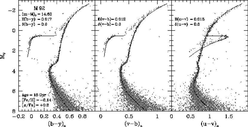
Figure 1: Various $uvby$ CMDs for the metal-poor globular cluster M 92 overlaid with a 15 Gyr, $\rm{[Fe/H]}=-2.14$ isochrone and ZAHB model (Bergbusch & VandenBerg, 2001). These models are transposed to the observed planes using our synthetic Strömgren colors and the bolometric corrections from Paper I. Reddening corrections (corresponding to $\rm{E{\it(B-V)}}=0.023$, Schlegel et al., 1998) are as indicated, and the adopted apparent distance modulus is based on the local Population II subgiant HD 140283. Only in the case of the $u-v$ data was an additional color shift applied to the observations (see footnote 6), aside from the reddening.

To begin our assessment of the quality of the computed Strömgren colors, we will examine the fits of isochrones to the various $uvby$ CMDs of the globular cluster M 92. Indeed, this same cluster played an important role in the testing of the BV(RI)_C transformations and bolometric corrections for extremely metal-poor stars in Paper I. In order to be consistent with Paper I, we will assume the same apparent distance modulus [$(m-M)_{V}=14.6$, Grundahl et al. 2000a] and reddening value [$\rm{E{\it(B-V)}}=0.023$, Schlegel et al. 1998] for the purpose of our analysis. Figure 1 presents the fit of a 15 Gyr isochrone and zero-age horizontal branch (ZAHB) model (Bergbusch & VandenBerg, 2001) for $\rm{[Fe/H]}=-2.14$, which is within $\pm 0.1$ dex of the values derived by Zinn & West and Carretta & Gratton, and [$\alpha$/Fe]$\,=+0.3$ (Carney, 1996) to the cluster data on three different Strömgren color-magnitude planes. Upon initial inspection, it is quite obvious that both the ZAHB model and the isochrone provide superb and consistent fits to the photometric data on all three CMDs from the tip of the red giant branch, through the turnoff region, and down to $M_{V}\approx 6$. Moreover, our interpretations of the cluster $uvby$ data is completely consistent with that obtained in Paper I where the same 15 Gyr isochrone was found to provide the best fit to the $B-V$ data for M 92 (see their Fig. 1) reported by Stetson & Harris (1988). To be sure, the cluster reddening, metallicity, and distance may not be exactly as we have assumed here, and the isochrones may be deficient in some respects, but to within all of these uncertainties, the isochrone fits to M 92 presented in Figure 1 seem to indicate that our synthetic $uvby$ color for $\rm{[Fe/H]}\leq-2.0$ are able to reproduce the observed photometry of old, metal-poor stars quite successfully.

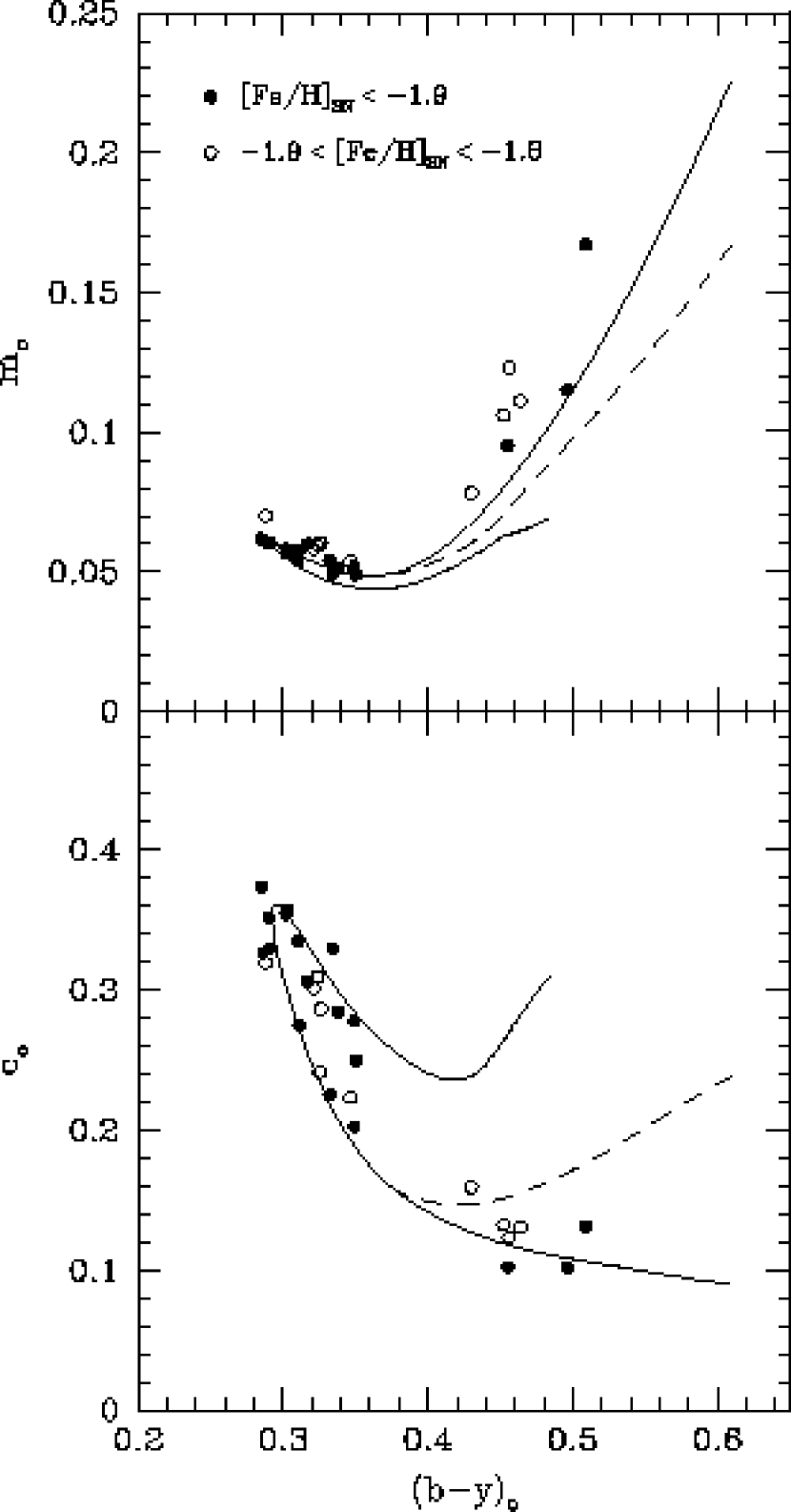
Figure 2: Color-color plots for a sample of metal-poor field stars with $uvby$ photometry from the survey of Schuster & Nissen (1988). The filled and open circles denote stars having photometric metallicity estimates from Schuster & Nissen (1989b) within the indicated ranges. The dashed and solid curves represent, in turn, the same 15 Gyr, $\rm{[Fe/H]}=-2.14$ isochrone used in the previous figure before and after corrections were applied to the synthetic $uvby$ color-temperature relations (see the text).

Apart from testing our synthetic $uvby$ colors for $\rm{[Fe/H]}\leq-2.0$ using cluster stars, we can also make use of a collection of field stars from the Schuster & Nissen (1988) study that have precise $uvby$ photometry and photometric metallicity and reddening estimates derived from the calibrations of Schuster & Nissen (1989a). In Figure 2 we compare, on two dereddened color-color planes, the same 15 Gyr, $\rm{[Fe/H]}=-2.14$ isochrone used above with the distribution of field stars having photometric metallicity estimates corresponding to $\rm{[Fe/H]}<-1.8$. As indicated by the dashed curves, this isochrone matches the warmer turnoff stars (those having $(b-y)_{o}\leq 0.4$) quite well, but it deviates from the loci defined by the few cooler dwarfs with $(b-y)_{o}\geq 0.4$. Based on these distance-independent plots, we have adjusted the synthetic $v-b$ and $u-v$ colors at $T_{\rm{eff}}\leq 5500\,$K and $\rm{log~{}g}\geq 3.5$ in order to alleviate these discrepancies. When the resultant empirically corrected transformations are employed, the 15 Gyr isochrone is given by the solid curves, which clearly provide much improved fits to the coolest field dwarfs. [Because the adjustments to the $v-b$ and $u-v$ colors are small in comparison with the breadth of the main-sequence photometry of M 92 at $(b-y)_{o}\sim 0.4$ (see Figure 1), they have no discernible impact on the quality of the isochrone fits to the cluster CMD. Note, as well, that the displacement of the open circles to the left of the solid curve in the top panel of Figure 2 is consistent with them being $\approx 0.25$ dex more metal rich than the isochrone.] We are thus led to conclude from Figure 2 that the synthetic colors corresponding to cool metal-poor dwarf stars are in error and that, in order for our $uvby$ colors to accurately describe the properties of such stars, some corrections to the transformations derived from model atmospheres are necessary, even at metallicities slightly below [Fe/H] $=-2.0$. (The corrections to the colors for metal-poor stars are discussed in more detail in Section 3.4. Possible causes of the discrepancies are discussed below.)

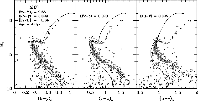
Figure 3: Same as Fig. 1 except for the open cluster M 67. The $solid~{}line$ plotted in each panel represents the same 4 Gyr, $\rm{[Fe/H]}=-0.04$ isochrone that provided the best fit to the broadband photometry of M 67 in Paper I. This isochrone, when transformed to the respective CMDs using our purely theoretical $uvby$ colors, obviously fails to reproduce the photometric data, particularly for $v-b$ and $u-v$.

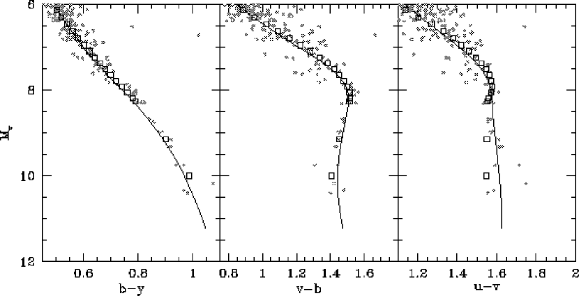
Figure 10: Various CMDs for K- and M-type dwarf stars in the solar neighborhood with $M_{V}$ values derived from their Hipparcos parallaxes and $uvby$ photometry from the EHO catalog. Only those stars with $\sigma_{\pi}$/$\pi\leq 0.1$ have been plotted. Our synthetic colors at $T_{\rm{eff}}\lesssim 4500$ K have been constrained by these data so that our ZAMS for $\rm{[Fe/H]}=0.0$ is given by the $solid~{}curve$ in each panel. As a check, we compare our ZAMS fit to the empirical standard relation for late-type dwarf stars (open squares) as derived by Olsen (1984).

Turning now to solar metallicity stars, we present in Figure 3 an analogous plot of $uvby$ CMDs, in this case for the open cluster M 67. Again, for the sake of consistency, we use the same values for the cluster distance, metallicity, reddening as those adopted in Paper I, which compared isochrones with the $B-V$, $V-R$, and $V-I$ CMDs of M 67. Unlike the previous example for M 92, however, the fits of our 4 Gyr, $\rm{[Fe/H]}=-0.04$ isochrone (from VandenBerg, Bergbusch, & Dowler, in preparation) to the cluster data exhibit some large discrepancies between the computed and observed CMDs. While the isochrone may be brought into better agreement with the cluster turnoff if the colors are shifted redward by small amounts depending on the index plotted, these shifts alone would obviously not be able to reconcile the disagreement in the main-sequence and giant-branch regions on the $v-b$ and $u-v$ planes. The cause of this difference is unlikely to be a problem with the temperature scale of the isochrone itself since Paper I has already shown that the $(B-V)$–$T_{\rm{eff}}$ relation predicted by the isochrone is in very good agreement with empirical relationships (see their Fig. 10). In addition, the luminosities and temperatures of the M 67 giant stars, as derived from $V-K$ photometry, are consistent with the predictions of the same 4 Gyr isochrone used here (see their Fig. 27).

There are a number of possible explanations for the differences seen in Figure 3. First, it is possible that the atomic and molecular line list used for calculating our synthetic spectra is not comprehensive enough to produce reliable Strömgren colors, particularly in the $u$ and $v$ pass bands where line blanketing is especially strong. Second, bands of the blue system of CN occur in the $u$, $v$ and $b$ filters are certainly strong enough to be readily visible in spectra of stars in the globular cluster 47 Tuc ($\rm{[Fe/H]}\approx-0.8$, Dickens, Bell, & Gustafsson, 1979). For simplicity, our spectral calculations do not allow for differences in CNO abundance. Third, line blocking depends upon the value adopted for the microturbulent velocity. Finally, Bell, Balachandran, & Bautista (2001) have found that, by incorporating bound-free transitions of Fe I into the SSG models, it is possible to obtain a better fit to the solar UV flux. The effects of this opacity source have not yet been included in our stellar models. Any combination of these factors could give rise to the mismatch between our synthetic colors and the observed M 67 data as well as the metal-poor field dwarfs in Figure 2.

To compensate for the problems in the $uvby$ colors mentioned above, it is clear that some corrections to our color–$T_{\rm{eff}}$ relations are necessary to bring them into better agreement with the observed data. Indeed, similar problems with the $BV(RI)_{C}$ transformations were dealt with in Paper I by applying suitable adjustments to the colors in order to satisfy empirical constraints imposed by both cluster and field stars. This semi-empirical approach will also be adopted here to correct our synthetic $uvby$ colors. In an effort to quantify the necessary corrections in the simplest and most straightforward manner possible, we have chosen to follow the methods of Houdashelt, Bell, & Sweigart (2000b, hereafter HBS2000) who calibrated their synthetic colors using a sample of field stars having precise $T_{\rm{eff}}$ estimates determined using the infrared flux method (IRFM).

Although HBS2000 developed their techniques as a means of semi-empirically correcting their synthetic $UBVRIJHK$ colors, their methods can be easily adapted to the present study provided that a large enough sample of field stars with $uvby$ photometry is available. The HBS2000 investigation employed a total sample of 101 field dwarf and giant stars taken from the studies of Bell & Gustafsson (1989, hereafter BG89) and Saxner & Hammärback (1985, hereafter SH85). We note, however, that this sample is mainly limited to stars with metallicities near solar and contains only two cool dwarfs with $T_{\rm{eff}}<5000\,$K. Given the significant discrepancies between the observed and computed M 67 CMDs in the vicinity of the lower main sequence on the $v-b$ and $u-v$ planes, such a small sample of cool dwarfs could pose a problem in deriving the correct calibrations for these indices towards cooler $T_{\rm{eff}}$’s. Therefore, we have supplemented the HBS2000 list with a much larger sample of stars with IRFM temperatures from the works of Alonso, Arribas, & Martínez-Roger (1996a, 1999, hereafter AAM96 and AAM99, respectively) that not only cover a broader range in metallicity, but also contain more cool dwarf stars. By combining the field-star lists from all of these studies, the final sample used here will not only be ideal for investigating the dependence of the color calibrations on $T_{\rm{eff}}$ and $\rm{log~{}g}$, but, with the increased range in metallicity, on $\rm{[Fe/H]}$ as well.

3.1 The Field Star Sample

While all of the studies mentioned above rely on the IRFM to determine $T_{\rm{eff}}$, a number of distinct differences exist between the methods and models employed by each. For example, both BG89 and SH85 use MARCS atmospheres to calibrate the ratio of bolometric to infrared flux, while AAM96 and AAM99 rely on the stellar models of Kurucz (1993). Moreover, the techniques for deriving the bolometric flux ($F_{\rm{bol}}$) differ in the fact that both BG89 and SH85 compute this quantity from a combination of 13-color, UV, and near-IR photometry, whereas AAM96/AAM99 rely solely on integrated $UBVRIJHK$ photometry. Therefore, some disagreement both in the computed $F_{\rm{bol}}$’s and IRFM temperatures could arise from these different treatments. For this reason, we feel it is important to check that the IRFM temperatures from these four separate studies are not only consistent with each other, but also that the stellar angular diameters, predicted from the $F_{\rm{bol}}$ and $T_{\rm{eff}}$ estimates, assuming $T_{\rm{eff}}\propto(F_{\rm{bol}}/\theta^{2})^{1/4}$, are in good agreement with recent interferometric estimates.

Table 1 presents a comparison of the $F_{\rm{bol}}$ and $T_{\rm{eff}}$ values for a number of stars in common between the different studies. The 34 dwarf and giant stars examined by both AAM96/AAM99 and BG89 differ by $\approx 6.2\%$ ($\pm 2.5\%$) in the mean $F_{\rm{bol}}$ value, or $\approx 65\,$K ($\pm 82$) in $<$$T_{\rm{eff}}$$>$, in the sense that the BG89 temperatures are hotter. However, one dwarf star in common between the two samples, HD 8086, deviates by more than 3$\sigma$ from the mean temperature. If this star is rejected from the sample, then the average $T_{\rm{eff}}$ difference is decreased to $-56\pm 60\,$K, with only a slight change in $F_{\rm{bol}}$ ($6.0\pm 0.2\%$). While this offset in $F_{\rm{bol}}$ is likely associated with the different methods used to calculate bolometric flux described above, the fact that the derived $T_{\rm{eff}}$’s are in agreement to within $\approx 60\,$K is quite reassuring when one considers that the uncertainties typically quoted for the IRFM range from 50 to 150 K. For AAM96/AAM99 and SH85 we find slightly better agreement: mean $F_{\rm{bol}}$ and $T_{\rm{eff}}$ differences of $2.5\pm 2.2\%$ and $8\pm 43\,$K, respectively, if the anomalous star HR 2085 is omitted from the consideration. We conclude from this analysis that the $T_{\rm{eff}}$’s computed by AAM96/AAM99 are consistent (to within the uncertainties of the IRFM itself) with those derived by SH85 and BG89.

Apart from confirming the consistency of the $T_{\rm{eff}}$’s derived in different studies, we must also ensure that the angular diameters computed from the IRFM temperatures and the $F_{\rm{bol}}$ values listed in Table 1 are in good agreement with those obtained from more direct interferometric estimates. To proceed, we make use of the angular diameters recently compiled by Nordgren et al. (1999, 2001, hereafter N99 and N01, respectively) for giant stars using the Naval Prototype Optical Interferometer. Table 2 presents the comparison between the N99/N01 measurements and those angular diameters inferred the results of BG89 and AAM99. While we opt to compare the angular diameters measurements, one can also compare the stellar radii once the distance to the star is known. For this reason, we have included the $Hipparcos$ parallax estimates for these stars so the reader can easily calculate and compare the stellar radii from the information given. It is important to note that the uniform-disk angular diameters determined from interferometry must be corrected for limb-darkening before they may be compared with those derived from the IRFM. N99/N01 accomplish this by applying correction factors between uniform disk and limb-darkened angular diameters from a set of coefficients derived by Claret, Diaz-Cordoves, & Gimenez (1995). The errors in $\theta$ quoted in Table 2 come directly from the N99 and N01 studies, whereas those computed from the IRFM temperatures were determined assuming a 5% uncertainty in $F_{\rm{bol}}$ and $\pm 100\,$K in $T_{\rm{eff}}$ for stars from both BG89 and AAM96/AAM99. The mean differences between the IRFM-derived angular diameters and those from interferometry are only $0.054\pm 0.108\,$mas and $-0.004\pm 0.094\,$mas for BG89 and AAM96/AAM99, respectively. Therefore, we can be quite confident that the IRFM temperature scale is correct.

In order to proceed with the calibrations of the synthetic Strömgren colors, we must first isolate stars from the lists of HBS2000 and AAM96/AAM99 that have both $uvby$ photometry and parallax estimates from the Hipparcos catalog. Our primary source of $uvby$ data for the color calibrations is the catalog of Hauck & Mermilliod (1998, hereafter HM98) which provides Strömgren photometry for more than 60000 stars. Although the HM98 catalog is ideal for our selection process, we are mindful of the fact that their final tabulated photometry often represents the weighted mean of several measurements compiled from different studies over the past four decades. Indeed, the data coming from such a large number of independent sources is sure to exhibit some inhomogeneities due to the different observational equipment and/or calibration techniques used by the various observers. This is particularly true for stars which lie in regions of the H-R diagram where the $uvby$ system is not well defined (i.e., extremely red and blue stars) and differences between different data sets can be as high as 0.1 mag for the $m_{1}$ and $c_{1}$ indices (see Olsen 1995 for a relevant discussion on this problem for late-type, metal-deficient giants). We do note, however, that the HM98 catalog is dominated by the photometric samples collected by Olsen (1983, 1984, 1993, 1994), Schuster & Nissen (1988), and Schuster, Parrao, & Contreras Martinez (1993). The $uvby$ data reported in these studies are particularly noteworthy since the authors generally used the same instrumentation and reduction procedures to produce their final calibrated photometry.

Our field star sample initially consisted of 559 stars that have both parallax and $uvby$ data from the Hipparcos and HM98 catalogs. Stars were subsequently excluded from this list if their IRFM temperatures are higher than 8000 K or below 4000 K, if they are flagged for variability or multiplicity in the Hipparcos catalog, or if their $uvby$ indices seem suspect when checked against their temperatures or spectral types. This culling process left us with 495 stars that were then examined individually for possible inhomogeneities in their $uvby$ photometry taken from HM98. The photometry for approximately 75% of these (365 stars) comes predominantly from the studies mentioned in the previous paragraph, and we are confident that their $uvby$ data are reliable enough for the color calibrations. In fact, no individual $b-y$, $m_{1}$, or $c_{1}$ measurement from these studies deviates by more than 0.02 mag from the mean values listed in HM98 for any of these 365 stars. As far as the remaining 25% of the sample is concerned, we have chosen to exclude them entirely from our analysis if any of their individual $uvby$ indices, taken from the various sources, differ by more than 0.05 mag from the HM98 means. Furthermore, any star having only one set of $uvby$ measurements was excluded if its colors do not correspond well (i.e., to within 0.05 mag) with those of stars with similar temperatures, gravities, and metallicities that were retained in our sample.

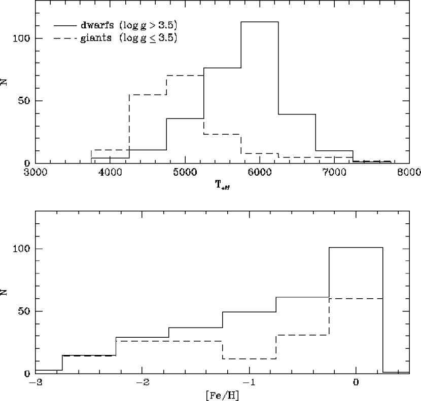
Figure 4: The distribution of our field star sample as a function of $T_{\rm{eff}}$ and $\rm{[Fe/H]}$. Note that $\rm{log~{}g}=3.5$ has been used to separate the dwarf- and giant-star distributions.

Our final sample consists of 478 field stars for which HBS2000 or AAM96/AAM99 provide estimates for $\rm{log~{}g}$ and $\rm{[Fe/H]}$. In some cases, however, these values may not necessarily be consistent with spectroscopic estimates. This is especially true for the stars listed by AAM96/AAM99, who assign only approximate values to the majority of their sample for the reason that $\rm{log~{}g}$ and $\rm{[Fe/H]}$ need only be accurate to within 0.5 dex and 0.3 dex, respectively, to obtain uncertainties in $T_{\rm{eff}}$ of $\approx 2\%$. Given the sensitivities of the Strömgren $m_{1}$ and $c_{1}$ indices to metal abundance and surface gravity, and the possible effects that uncertainties in these values may have in the subsequent color calibrations, we have chosen to extract more precise spectroscopic values from the $\rm{[Fe/H]}$ catalog of Cayrel de Strobel, Soubiran, & Ralite (2001). For cases where the catalog provides more than one set of estimates for each star, we adopt the median values for $\rm{log~{}g}$ and $\rm{[Fe/H]}$. Though the majority of these stars are relatively nearby, some might be heavily reddened by local interstellar dust clouds. For this reason, we adopt the E$(B-V)$ values given by AAM96/AAM99, while reddening estimates for stars from HBS2000 are derived from the extinction maps of Schlegel et al. (1998) and corrected for distance using the expression [1$-$exp($-$$|$$d$ sin $b$$|$/$h$)], where $d$ is the star’s distance (as determined from the Hipparcos parallaxes), $b$ its galactic latitude, and $h$ the dust scale-height (assumed to be 125 pc, Bonifacio, Caffau, & Molaro, 2000). The final composite list of stars in our sample is given in Table 3, and histograms illustrating their distribution as a function of $T_{\rm{eff}}$ and $\rm{[Fe/H]}$ are shown in Figure 4.

3.2 Color Corrections at [Fe/H] = 0.0

Given that a sizable fraction ($\sim 35\%$) of the field stars in our sample have metallicities within $\pm 0.25$ dex of solar, they provide an excellent subset in which to determine what corrections to the colors at $\rm{[Fe/H]}=0.0$ are needed to bring them into better agreement with the observations. In this section we aim to follow the methods of HBS2000 by deriving corrections to synthetic colors based on simple polynomial fits to the distribution of synthetic versus observed colors for a sample of field stars with well-determined physical parameters.

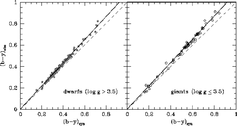
Figure 5: The synthetic vs. observed $b-y$ photometry for field stars listed in Table 3 with metallicities near solar (i.e., $-0.25\leq\rm{[Fe/H]}\leq+0.25$). The left-hand panel plots all dwarfs from the sample with $\rm{log~{}g}>3.5$ whereas the $open~{}circles$ in the right-hand panel indicate giants with $\rm{log~{}g}\leq 3.5$. The $solid~{}lines$ represent the linear, least-squares fits to the distribution of dwarfs and giants in each panel while the dashed lines represent the lines of equality between the observed and synthetic colors. These fitted relations are used to correct the synthetic $b-y$ colors to bring them into better agreement with the observed photometry.

We begin with the calibration of the $b-y$ index. In this case, as well as the calibrations for the other Strömgren colors that follow, a synthetic index for each star is determined from direct interpolation within our color grid assuming the $T_{\rm{eff}}$, $\rm{log~{}g}$, and $\rm{[Fe/H]}$ values listed in Table 3. This synthetic color is then plotted against its observed, dereddened counterpart for all stars in the sample that fall within $-0.25\leq\rm{[Fe/H]}\leq+0.25$ in order to establish the calibration of the model colors at $\rm{[Fe/H]}=0.0$. Figure 5 presents such a plot for the $b-y$ index with dwarfs and giant stars separated into different panels as a means of checking for possible differences between stars of different gravity. Inspection of the figure reveals that the synthetic colors for both the dwarfs and giants exhibit noticeable systematic deviations from equality (dashed line) towards cooler temperatures. If simple linear, least-squares fits are derived for each of the two sets separately, we indeed find that the slopes are greater than unity (see Table 4). Furthermore, a single linear fit involving the dwarfs and the giants together show that they follow very nearly the same trend as those obtained when they are treated separately to within the errors of the fitted lines. Based on this result, we conclude that our synthetic $b-y$ colors at $\rm{[Fe/H]}=0.0$ can be suitably corrected to match the observed field-star photometry using a single linear calibration.

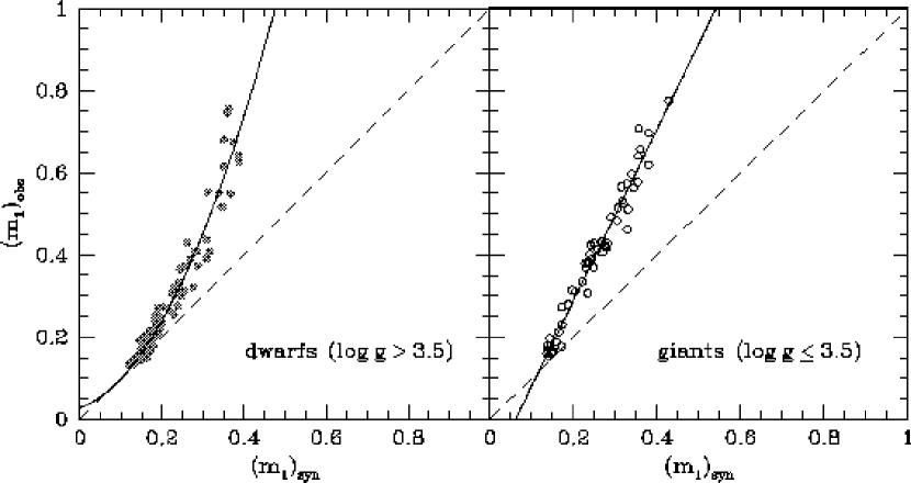
Figure 6: Same as Figure 5 except for the $m_{1}$ index. In this case, the dwarf stars are best fitted using a second-order polynomial, whereas the giants follow the indicated linear relation.

In Figure 6 we present a plot comparing the synthetic versus observed $m_{1}$ colors for the same subset of stars considered in Figure 5. In this case the synthetic colors exhibit substantial deviations from their observed counterparts for both the dwarfs and the giants. Unlike the $b-y$ index, however, the dwarfs appear to follow a somewhat different trend than the giants, and a single linear calibration would not be satisfactory. Indeed, the interpretation of this diagram is more complex that that of Figure 5 in the sense that $m_{1}$ is sensitive to the abundances of some individual elements and isotopes (e.g., C, N, and ¹²C/¹³C) as well as the overall metal abundance, while $b-y$ depends primarily on temperature. However, since these deviations in Figure 6 appear to be consistent with the discrepancies between our 4 Gyr isochrone and the $v-b$ CMD for M 67 [recall that $m_{1}=(v-b)-(b-y)$] in Figure 3, we proceed to correct the $m_{1}$ colors using the same procedure as that employed for the $b-y$ index. We fit the dwarf-star distribution using a second-order polynomial, whereas a linear relation is derived for the giants. The corresponding coefficients of these fits are again given in Table 4. This type of calibration for the dwarf-star $m_{1}$ colors is not unreasonable. For comparison, some of the synthetic broadband colors computed by HBS2000, particularly the $B-V$ and $V-I$ indices, exhibited large deviations among the coolest dwarfs in their sample. Their solution involved a separate cool-dwarf calibration that deviated from their derived fit to the warmer dwarfs at a temperature of 5000 K. We have similarly investigated if two separate linear calibrations, one for warm dwarfs and another for cool dwarfs using 5000 K as the dividing temperature, would adequately correct the $m_{1}$ colors and found that the cool dwarfs appear to be “over corrected” in a sense that their calibrated colors extend too far to the red to adequately fit the $v-b$ (and $m_{1}$) photometry on the lower main sequence of M 67. Therefore, the original second-order polynomial is used to correct the $m_{1}$ colors for $\rm{log~{}g}>3.5$, and we have taken great care to smoothly meld these calibrated dwarf-star colors to those for the giants at $\rm{log~{}g}=3.5$.

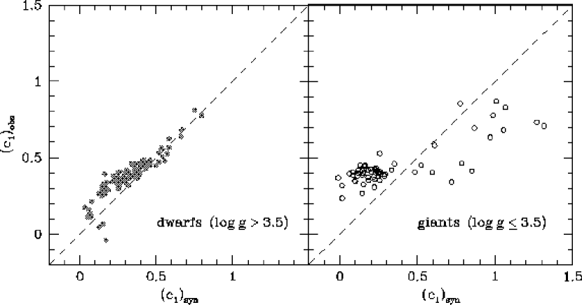
Figure 7: Same as Figures 5 and 6 except for the $c_{1}$ index. Note that both the dwarfs and giants do not appear to follow any specific trend, either linear or polynomial, and as a result, it is not possible to derive a satisfactory calibration for $c_{1}$ from such plots.

The final index left to calibrate is the Strömgren $c_{1}$ index. Upon inspection of Figure 7, however, it would appear that this index poses even more of a problem to calibrate. While the dwarf stars are fairly well defined in the plot, the giants show an appreciable scatter at large $c_{1}$ values and do not seem to follow any specific trend. As with the $m_{1}$ index, the correct interpretation of Figure 7 depends on the sensitivity of $c_{1}$ to the effects of surface gravity, chemical abundance, $and$ temperature. Moreover, the $u-v$ component of $c_{1}$ is not a monotonic function of temperature. Some additional factors that may contribute to the problems with the $c_{1}$ index could be missing absorption lines and/or the exclusion of the aforementioned Fe I opacity source in our SSG spectra. In addition, as mentioned in the previous section, the scatter at large $c_{1}$ values for the giants could be associated with inhomogeneities in the HM98 catalog due to the fact that the Strömgren system is not well established for these types of stars. However, we have been careful to exclude stars if their photometry seems suspect, and we are confident that the scatter seen in the right-hand panel of Figure 7 is real. To complicate matters further, Grundahl et al. (2000b) first cited evidence that the $c_{1}$ colors of RGB stars in globular clusters exhibit a rather large scatter that is much greater than the photometric uncertainties. This $c_{1}$ scatter has since been confirmed to be present among RGB stars in all 21 globular clusters surveyed in the Grundahl program (Grundahl et al., in preparation). This effect has been interpreted as star-to-star differences in the abundance of nitrogen (Grundahl et al., 2002a). Since numerous NH lines lie within the Strömgren $u$ filter, the $c_{1}$ color of any star with an abnormal abundance of nitrogen will be different from that of one with a normal abundance. As a result, our synthetic $c_{1}$ colors, which are derived from MARCS/SSG models assuming scaled-solar abundances, cannot be expected to reproduce the observed colors of field stars having abnormal abundances of nitrogen.

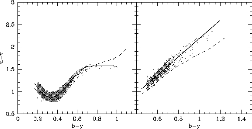
Figure 8: Two ($b-y$, $u-v$) diagrams for a sample of dwarf and giant stars (left- and right-hand panels, respectively) having parallax estimates from Hipparcos and $uvby$ data from the EHO catalog. The $solid~{}lines$ indicate the relationships derived to fit the distribution in the photometric data and are used to correct our synthetic $u-v$ colors. Dashed lines represent the locus of a solar metallicity ZAMS model (for the dwarfs) and the giant branch from our 4 Gyr isochrone before corrections to the $u-v$ colors are applied.

Given the obvious lack of agreement between the synthetic and observed indices in Figure 7, it is clearly very difficult to derive any calibrations that would adequately correct the dwarf and giant $c_{1}$ colors. Consequently, we have explored alternate techniques of correcting the $c_{1}$ colors for solar-metallicity models, and found that the most straightforward way involved working with the distribution of field dwarf and giant stars which have $uvby$ photometry and parallax estimates from Hipparcos on the ($b-y$, $u-v$) plane. We choose to deal predominantly with the synthetic $u-v$ colors rather than $c_{1}$ itself since the latter includes a combination of both the $u-v$ and $v-b$ indices [recall that $c_{1}=(u-v)-(v-b)$]. As the $v-b$ and $b-y$ indices have already been calibrated, we only need to investigate what corrections are required to fix the synthetic $u-v$ colors. In Figure 8 we present the color-color plots for those dwarfs and giants with accurate parallax estimates from Hipparcos. Rather than rely on the HM98 catalog as our source of photometry for this analysis, we have instead chosen to extract the data from a catalog of accurate and homogeneous $uvbyH\beta$ photometry recently compiled by E. H. Olsen (private communication) from his published samples Olsen (1983, 1984, 1993, 1994). This catalog, hereafter referred to as the EHO catalog, is comprised of almost 30000 stars in the northern and southern hemispheres, all of which are reduced carefully to the standard $uvby$ system. Since these Hipparcos stars are relatively nearby, we can safely neglect the effects of reddening, and assume they all have metallicities near solar. To ensure that the purest sample of dwarfs and giants are presented in both panels, we impose cuts on the data based on the star’s absolute magnitude and $b-y$ color. For instance, all cool dwarf stars plotted in the left-hand panel of Figure 8 have $M_{V}\geq 10\;(b-y)$ and $b-y\geq 0.2$ (corresponding to $T_{\rm{eff}}\lesssim 7250\,$K), and we have isolated the giant stars to $M_{V}\leq 4.5$ and $b-y\geq 0.5$ ($T_{\rm{eff}}\lesssim 5250\,$K). In the case of the dwarfs a 6th order polynomial, using $b-y$ as the independent variable, is used to fit the distribution of data between $0.2\leq\,b-y\,\leq 1.0$, while the giant stars are fit using a simple linear relation for $0.5\leq\,b-y\,\leq 1.2$.

These relations, which are indicated in each panel of Figure 8 by a solid curve, are subsequently used to correct our synthetic $u-v$ colors. In the case of the dwarf stars, the synthetic $u-v$ colors predicted from a solar-metallicity ZAMS model (dashed curve) are forced into agreement with the polynomial fit. In general this meant applying redward shifts ranging approximately from 0.01 to 0.1 mag in the $u-v$ colors for $0.3\leq\,b-y\,\leq 0.7$, whereas a combination of positive and negative corrections were required to match the distribution of the cool dwarf stars at $b-y\gtrsim 0.7$. Similarly, the $u-v$ colors corresponding to the giants in the right-hand panel are brought into agreement with the derived linear relation by using the color predictions from the giant branch of the 4 Gyr, $\rm{[Fe/H]}=-0.04$ isochrone (dashed curve). These corrections for the giants were generally much larger than for the dwarfs and ranged from +0.15 to +0.25 depending on $b-y$ color.

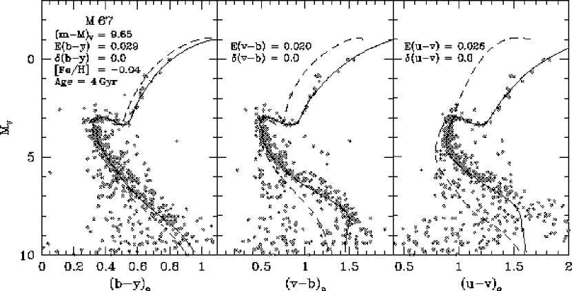
Figure 9: Same as Figure 3 except the 4 Gyr isochrone (solid lines) has been transformed to the color-magnitude planes using our newly calibrated $uvby$ colors while the dashed lines represent the uncalibrated isochrone.

With the synthetic Strömgren colors at $\rm{[Fe/H]}=0.0$ now placed onto the observational system as the result of our analysis of field stars, we can again assess how well we can reproduce the various CMDs of M 67. Figure 9 provides the revised fits of the same 4 Gyr isochrone used in Figure 3, except that the transformation to the observed planes is accomplished using the calibrated $uvby$ colors. (Note that the same reddening and distance are adopted as in Figure 3.) The uncalibrated and calibrated isochrones are shown as dashed and solid lines, respectively. Overall, the fits to the various M 67 CMDs using the calibrated colors have been quite dramatically improved as compared with those using the purely theoretical indices. Importantly, the fits to all three CMDs now show excellent consistency with each other as well as with the interpretations of the $B-V$, $V-R$, and $V-I$ CMDs of M 67 discussed in Paper I.

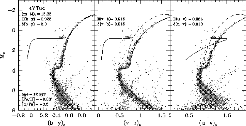
Figure 17: As in Fig. 16, except for the globular cluster 47 Tuc (NGC 104). Note that the apparent distance modulus and reddening values are identical to those adopted in Paper I. Our 12 Gyr, $\rm{[Fe/H]}=-0.83$ isochrone and ZAHB model are overlaid on the cluster photometry.

It worth noting that the preceding calibrations of the synthetic colors are technically valid for those dwarf and giant star models with $\rm{[Fe/H]}=0.0$ and $4000\leq T_{\rm{eff}}\leq 8000\,$K since we have employed only solar-metallicity field stars that fall within this temperature range. While a detailed discussion of the corrections made to models with metal abundances other than solar is deferred until later, we make a few remarks here concerning the color corrections for $T_{\rm{eff}}$’s outside this range. As mentioned in Section 2, we have adopted the synthetic $uvby$ colors of CGK97 for $T_{\rm{eff}}>8000\,$K and have made small corrections (typically less than 0.01$-$0.02 mag depending on the index) to our synthetic colors at temperatures of 7500, 7750, and 8000 K in order to meld our grid smoothly with theirs. At temperatures below 4000 K, we apply corrections to the colors at $\rm{[Fe/H]}=0.0$ in an effort to match the CMDs for a sample of extremely red field dwarf stars from the EHO and Hipparcos catalogs. In Figure 10 we present the fits of a ZAMS model having $\rm{[Fe/H]}=0.0$ which has been transformed to the indicated CMDs using the final corrected colors (solid curve) and overlayed on the photometry for stars having extremely precise parallaxes (i.e., $\sigma_{\pi}/\pi\leq 0.1$). This technique is similar to that presented in Paper I, which relied upon a large number of Gliese catalog stars to constrain the $BV(RI)_{C}$ color–$T_{\rm{eff}}$ relations down to $M_{V}\sim 13$ (see their Fig. 17). However, very few of these low-mass Gliese stars have observed $uvby$ data available in the EHO catalog and we can only define our color transformations accurately down to $M_{V}\approx 10.5$ ($T_{\rm{eff}}\approx 3500\,$K). Therefore, the corrections applied to the colors at 3000 and 3250 K are somewhat more uncertain since we do not have any additional data for extremely low mass stars that would help to better constrain them. As an additional check of our color corrections we plot the $uvby$ standard relation for late-type dwarf stars derived by Olsen (1984) as open squares in each panel of Figure 10. Overall, the ZAMS and the standard relation agree quite well in all three panels except at $M_{V}>9$ in the $u-v$ plot where the Olsen trend appears to deviate from the field star distribution towards the blue. (An implicit assumption here is that the $T_{\rm eff}$ scale of the ZAMS models for very low mass stars is accurate. For some discussion of the reliability of this aspect of these models, reference should be made to Paper I.)

3.3 The Calibrated Colors and Hipparcos Field Stars

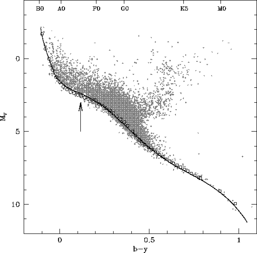
Figure 11: The ($b-y$, $M_{V}$) diagram for field stars from the Hipparcos catalog having accurate parallax estimates (i.e., $\sigma_{\pi}/\pi\leq 0.1$) and available $uvby$ photometry from EHO catalog. Two empirical standard relations corresponding to warm dwarfs (Philip & Egret, 1980, $open~{}circles$) and cool dwarfs (Olsen, 1984, $open~{}squares$) are also plotted on the data to represent the approximate location of solar metallicity dwarf stars in Strömgren color-magnitude space. A ZAMS locus for $\rm{[Fe/H]}=0.0$ is transformed to the CMD using our newly calibrated $b-y$ colors (and bolometric corrections from Paper I) and shown as a solid line. The vertical arrow located at $b-y\approx 0.1$ denotes where our cool star colors have been melded with those of CGK97 at a temperature of 8000 K.

To further illustrate the accuracy of our newly calibrated $uvby$ colors for solar-metallicity stars, we demonstrate their ability to reproduce the observed distribution of field stars on a variety of Strömgren color-magnitude and color-color planes. For this investigation we again make use of the sample of nearby Hipparcos stars described in the previous section. Since this sample is comprised primarily of stars with near-solar abundance lying close to the main sequence, a ZAMS model for $\rm{[Fe/H]}=0.0$ is an appropriate locus to compare with the $uvby$ data. Figure 11 presents the overlay of this ZAMS onto the field-star photometry in the ($b-y$, $M_{V}$) plane. As mentioned earlier, the Strömgren photometry for each star was taken directly from the EHO catalog of homogeneous $uvby$ data, while the broadband V magnitudes, which were used to derive $M_{V}$, are from the original Hipparcos photometric catalog. In addition to the field-star data, we have plotted two empirical standard relations as defined by Philip & Egret (1980, $open~{}circles$) for O$-$F-type main-sequence stars and by Olsen (1984, $open~{}squares$) for G$-$M dwarfs. The vertical arrow located at $(b-y)\sim 0.1$ indicates the region where our calibrated color-temperature relations have been joined with those of CGK97 at a temperature corresponding to 8000 K. Overall, the match to both the photometric data as well as the empirically defined standard relations is quite good.

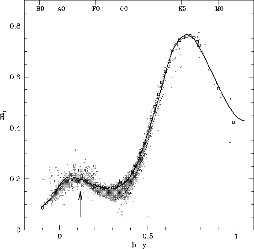
Figure 12: As in Fig. 11, except that the observations are plotted on the ($b-y$, $m_{1}$) diagram. The $dotted~{}line$ below the solar metallicity ZAMS denotes the location of an additional ZAMS model having $\rm{[Fe/H]}=-0.5$.

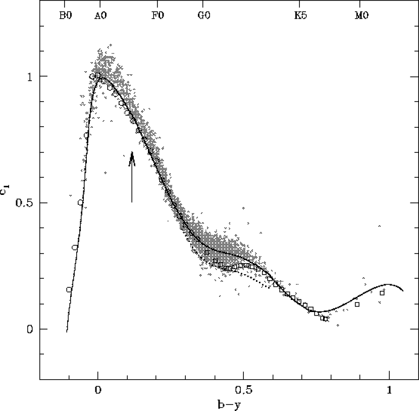
Figure 13: As in Fig. 12, except that the observations are plotted on the ($b-y$, $c_{1}$) plane.

In Figures 12 and 13 the same solar metallicity ZAMS is transposed onto the ($b-y$, $m_{1}$) and ($b-y$, $c_{1}$) color planes to illustrate how well it is able to reproduce the observed stellar distributions. For the former plot, the standard relation of Philip & Egret has been adjusted by $-$0.01 in $m_{1}$ to better match the photometric means derived from main-sequence spectral types (see Fig. 2 of Philip & Egret, 1983). Overall, the ZAMS locus agrees quite well with the observations over a broad range in color. We again stress the fact that, for $b-y\lesssim 0.1$, the colors are purely theoretical with no corrections applied. This type of diagram illustrates the unique sensitivity of the $m_{1}$ index to chemical abundance in F- and G-type dwarf stars through a noticeable spread in the $m_{1}$ colors at $0.2\leq\,b-y\,\leq 0.5$. While the location of our solar-metallicity ZAMS locus corresponds well with the turnover in the standard relations and the stellar data in this range, we have included an additional ZAMS having $\rm{[Fe/H]}=-0.5$ (dotted line) to show that the majority of dwarfs with slightly bluer $m_{1}$ colors have metallicities up to 0.5 dex less than solar. Indeed, our $\rm{[Fe/H]}=-0.5$ ZAMS follows the lower bound of the stellar distribution for the F- and G-type dwarfs quite well in Figure 12 with the few stars having slightly bluer $m_{1}$ values at $b-y\approx 0.35$ likely being even more metal poor.

Upon inspection of the ($b-y$, $c_{1}$) diagram in Figure 13, there is a difference between the Olsen standard relation and the ZAMS both at extremely cool temperatures and in the color range corresponding to G-type stars. While the mismatch at the cool end of the main sequence is most likely due to the small number of M dwarfs used to define the Olsen trend and has already been noted in Figure 10, the reason for the difference seen in the G dwarfs is not immediately apparent. Although the magnitude of this discrepancy is quite large ($\sim 0.04$$-$$0.05\,$mag), we suggest that the explanation lies in the fact that the $c_{1}$ index exhibits some sensitivity to star-to-star variations in metal abundance within this temperature range — which may explain the rather large spread in $c_{1}$ colors at $0.3\leq\,b-y\,\leq 0.5$. In support of this argument, the same $\rm{[Fe/H]}=-0.5$ ZAMS from the previous figure is again plotted to show that it defines the lower distribution of stars very well for the F- and G-type dwarfs. It would appear that slightly more metal-poor stars are predicted to lie up to 0.07 mag below the trend defined by the solar-metallicity dwarfs.

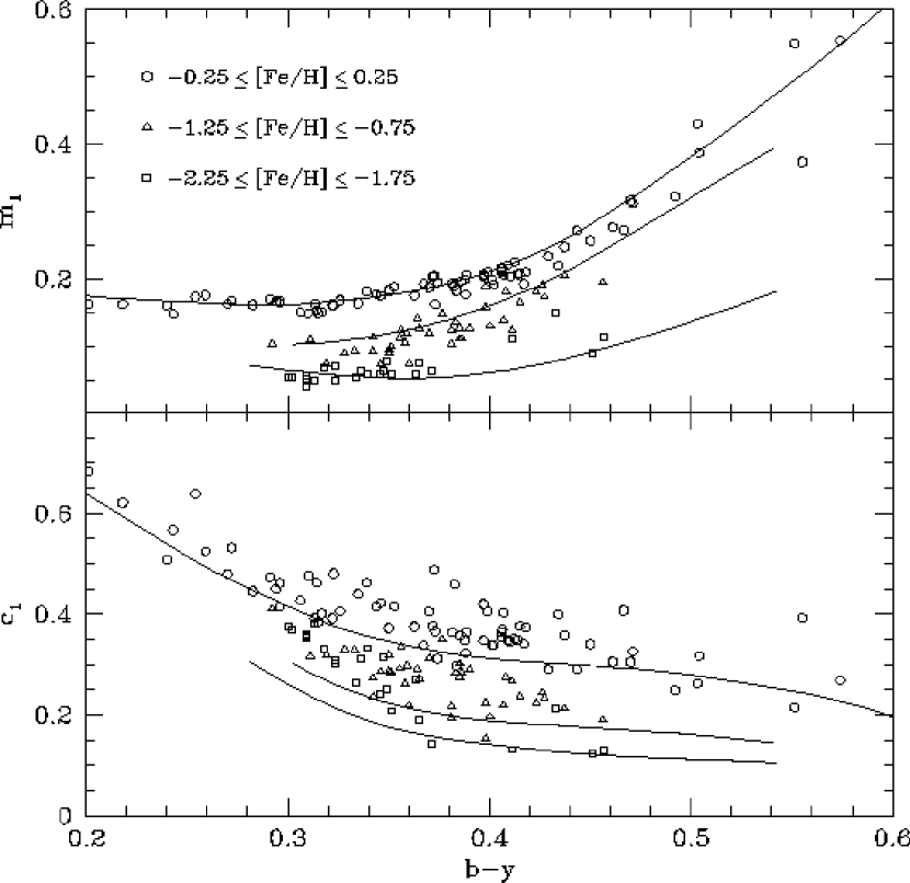
Figure 14: Two color-color diagrams for the field star data from Table 3 separated according to their metallicity values, as denoted by the different symbols. Three ZAMS models having $\rm{[Fe/H]}=0.0$, $-1.0$, $-2.0$ (in order of decreasing $m_{1}$ and $c_{1}$) are represented by solid lines.

To further expand on this, Figure 14 illustrates the metallicity dependence of the Strömgren $m_{1}$ and $c_{1}$ colors for F- and G-type dwarfs. For this purpose we have plotted only those field dwarfs stars in Table 3 that have metallicity estimates. The stars in each panel are divided into separate metallicity bins as indicated by the different symbols and overlaid with three ZAMS models for $\rm{[Fe/H]}=0.0$, $-1.0$, and $-2.0$ (in the order of decreasing $m_{1}$ and $c_{1}$). Recall that the colors employed for $\rm{[Fe/H]}=0.0$ ZAMS have been calibrated as described in the previous section. While we defer the discussion of corrections to the colors made at other metallicities until the next section, it is worth mentioning that the corrections to the $uvby$ colors towards cooler effective temperatures (i.e., $T_{\rm{eff}}\leq 5500\,$K) at $\rm{[Fe/H]}=-1.0$ and $-2.0$ are primarily constrained by the metal-poor field stars from the Schuster & Nissen (1989b) sample (see Figure 2) as well as the lower main sequences of the globular clusters M 3 and 47 Tuc. It is immediately obvious that stars with differing chemical composition exhibit a rather large photometric spread both in $m_{1}$ and $c_{1}$ at $b-y$ colors between 0.3 and 0.5. In the case of the bottom panel of Figure 14, all three of our ZAMS models do an excellent job of reproducing the lower bound to the distribution of dwarf stars in their respective metallicity bins. This is to be expected since a star that has evolved away from the main sequence would have a larger $c_{1}$ index than another star of the same temperature and metallicity but showing little evolution. Given this evidence, it would seem that Olsen’s calibration may have been based on stars with slightly less than solar abundances in this regime rather than actual solar-metallicity main-sequence stars.

3.4 Color Corrections at [Fe/H]$\,\leq\,$–0.5 and [Fe/H] = +0.5

Based on the analysis presented so far, we conclude that our calibrated $uvby$ colors at $\rm{[Fe/H]}=0.0$ are able to provide both accurate and consistent interpretations of the observed photometry for dwarf and giant stars having metallicities near the solar value. Moreover, our colors appear to do a reasonable job of reproducing the observed photometry of metal-poor turnoff and giant stars (see Figure 1) and our adopted color transformations in these temperature and gravity regimes for $\rm{[Fe/H]}\leq-2.0$ remain purely theoretical. However, from the evidence presented in Figure 2, it seems clear that some adjustment to the cool dwarf-star colors at extremely low metallicities is necessary in order to obtain consistency with the field-star data. To be more specific, we chose to keep all of the $b-y$ predictions at $\rm{[Fe/H]}\leq-2.0$ purely theoretical, but to apply some corrections to the $v-b$ and $u-v$ colors at temperatures and gravities relevant to cool dwarfs (i.e., at $T_{\rm{eff}}\leq 5500\,$K and $\rm{log~{}g}\geq 3.5$) to secure a better fit of the $\rm{[Fe/H]}=-2.14$ isochrone to the data. In general, this meant iteratively forcing the $v-b$ colors redder (i.e., making them more positive) and the $u-v$ colors bluer (i.e., more negative) by increasing amounts towards cooler temperatures. The justification for this admittedly ad hoc procedure is simply that such adjustments are required to satisfy the constraints imposed by the empirical data available to us at this time. Indeed, we are quite confident that our $uvby$ color transformations for $\rm{[Fe/H]}\leq-2.0$ are able to reproduce the observed photometry for metal-poor stars across a wide range in temperature and gravity. Since it was necessary to make some corrections to the synthetic colors for very metal-deficient stars and at $\rm{[Fe/H]}=0.0$, it is to be expected that they will be necessary for essentially all [Fe/H] values.

In order to quantify what color corrections are necessary at intermediate metallicities (i.e., $-1.5\leq\rm{[Fe/H]}\leq-0.5$), we have investigated if the same techniques employed earlier for the correction of the colors at $\rm{[Fe/H]}=0.0$ might continue to be applicable. However, the decrease in the number of stars from Table 3 having lower metallicity values, combined with their limited ranges in color (particularly for the dwarf stars), led us to conclude that there is not enough information from the field-star sample to derive the necessary calibrations adequately. Therefore, we choose not to rely on our field-stars to calibrate the colors for intermediate metallicities, but rather employ them later to test the relevancy of the corrections to the $uvby$ colors we derive for $-1.5\leq\rm{[Fe/H]}\leq-0.5$ described below.

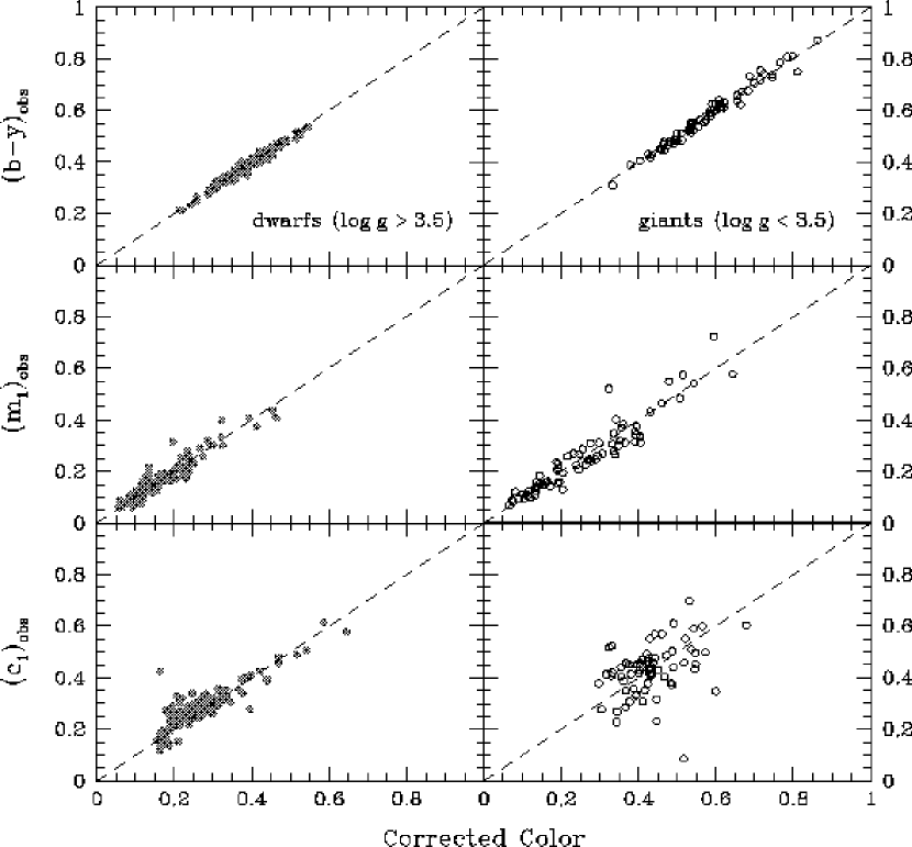
Figure 15: Plots of the corrected versus observed colors for dwarfs and giants with intermediate metallicities (i.e., $-1.75\leq\rm{[Fe/H]}\leq-0.25$) from our field star sample. The dashed line indicates the line of equality.

Since we have found that no corrections whatsoever are necessary for the synthetic $uvby$ colors with $\rm{[Fe/H]}\leq-2.0$ towards warmer temperatures ($T_{\rm{eff}}>5500\,$K) or lower gravities ($\rm{log~{}g}<3.5$), we have simply chosen to assume that the required adjustments to the color transformations at intermediate metallicities in these same temperature and gravity regimes are some fraction of those applied at $\rm{[Fe/H]}=0.0$. In particular, we assume that the size of this fraction scales linearly as a function of $\rm{[Fe/H]}$. For instance, the corrections applied to the synthetic colors at $\rm{[Fe/H]}=-0.5$ and $-1.0$ for a particular temperature and gravity correspond to $one$-$quarter$ and $one$-$half$ of the corrections that are required at $\rm{[Fe/H]}=0.0$ for the same $T_{\rm{eff}}$ and $\rm{log~{}g}$. For cool dwarf stars, however, it was necessary to correct the $v-b$ and $u-v$ colors in a similar fashion as those for $\rm{[Fe/H]}\leq-2.0$; i.e., we have used the $uvby$ data available to us from the metal-poor field-star sample of Schuster & Nissen, together with the precise $uvby$ photometry for the globular clusters M 3 and 47 Tuc, to derive the transformations that yield the best possible matches to the empirical data for cool cluster and field dwarfs having $-1.5\leq\rm{[Fe/H]}\leq-0.5$. Again, while our approach is ad hoc, we remark that when the synthetic colors are corrected in this way, they seem to agree quite well with observed colors for stars from our sample. This is illustrated in Figure 15, which plots the $calibrated$ versus observed colors of all the dwarfs and giants in Table 3 having $-1.75\leq\rm{[Fe/H]}\leq-0.25$. There are clearly no systematic differences or inconsistencies between the corrected and observed colors within this metallicity range, which lends considerable support to our technique of scaling the corrections as a function of $\rm{[Fe/H]}$ as well as the adjustments made for cooler dwarf stars.

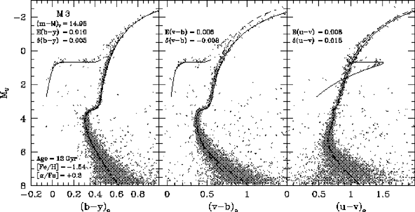
Figure 16: Various $uvby$ CMDs for the globular cluster M 3 overlaid with a 13 Gyr, $\rm{[Fe/H]}=-1.54$ isochrone and consistent ZAHB model. The indicated reddening is taken from the dust maps of Schlegel et al. while the apparent distance modulus is derived from the fit of the ZAHB model to the lower distribution of stars on the horizontal branch. The uncalibrated isochrone is represented by a $dashed~{}line$ in each panel.

Further illustrations of the accuracy of the corrected colors for intermediate metallicities are given in Figure 16 and 17, which present comparisons of the CMDs for M 3 and 47 Tuc with relevant isochrones and ZAHB models. According to Kraft & Ivans (2003), the iron abundance of M 3 is between $\rm{[Fe/H]}=-1.50$ and $-1.58$, which is within $\approx 0.1$ dex of the Zinn & West (1984) estimate. There seems to be general agreement that 47 Tuc has $\rm{[Fe/H]}=-0.75\pm 0.1$ (see Kraft & Ivans, 2003; Zinn & West, 1984; Carretta & Gratton, 1997). Isochrones for metallicities within these ranges provide very good fits to the cluster data if the foreground reddenings are taken from the Schlegel et al. dust maps, and the adopted distances are based on fits of ZAHB models to the lower bounds of the respective distributions of horizontal-branch stars. Of these two clusters, only 47 Tuc was considered in Paper I, and the match reported therein of the same isochrone used here to the $B-V$ fiducial derived by Hesser et al. (1987) is completely consistent with those shown in Figure 17. This is particularly encouraging because cluster data has played no role whatsoever in our determination of the corrections to the synthetic $uvby$ transformations at temperatures corresponding to the turnoff stars in metal-poor globular clusters (i.e., $T_{\rm{eff}}>5500\,$K), and yet we find essentially the same interpretation of the M 92 and 47 Tuc CMDs as in Paper I. This consistency provides a strong argument that the color transformations that have been derived in both investigations, as well as the model $T_{\rm{eff}}$ scale, are realistic. It is also evident that the size of the color adjustments increases with increasing $\rm{[Fe/H]}$ — note the differences between the $dashed$ and $solid$ curves, which represent the $uncalibrated$ and $calibrated$ isochrones, respectively. The same thing was found in Paper I. Although we have applied small shifts to some of the colors to obtain consistent fits to the turnoff data on the various color planes, it is not possible to say at this time whether they are due to small problems with the photometric zero-points, the adopted cluster parameters, the isochrones, or the color-temperature relations.

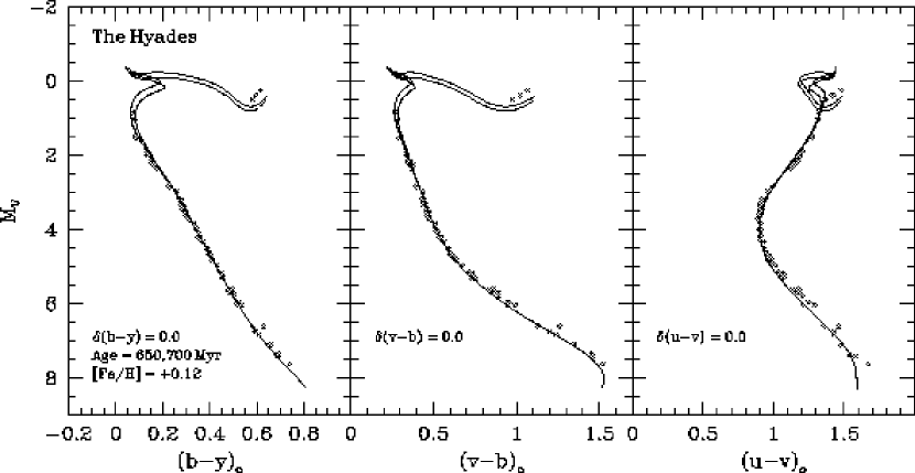
Figure 18: Strömgren CMDs for a sample of 77 “high-fidelity” single stars in the Hyades open cluster. Two isochrones having ages of 650 and 700 Myr with $\rm{[Fe/H]}=+0.12$ are overlaid on the photometric data. Note that the absolute magnitude for each star was derived from Hipparcos secular parallaxes by de Bruijne, Hoogerwerf, & de Zeeuw (2001).

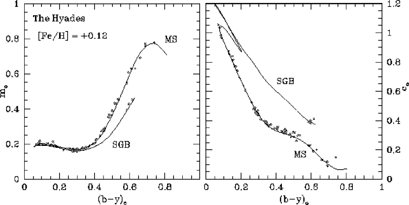
Figure 19: Strömgren color-color diagrams for the same sample of Hyades stars from the previous figure overplotted with a 700 Myr, $\rm{[Fe/H]}=+0.12$ isochrone. The main-sequence (MS) and subgiant (SGB) segments of the isochrone are labeled.

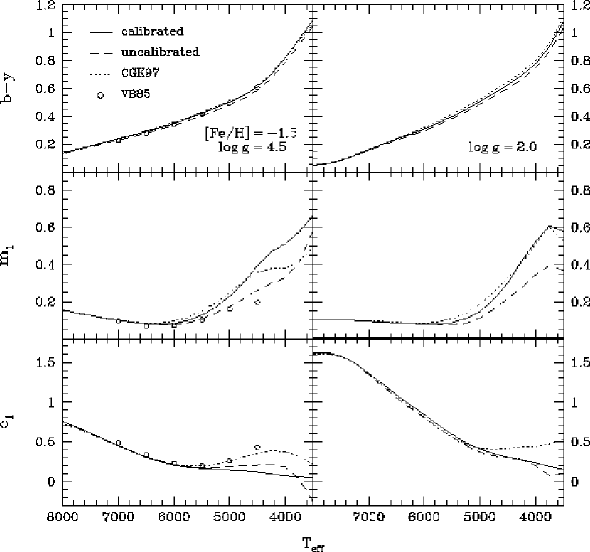
Figure 21: A comparison of synthetic color-temperature relations for $\rm{log~{}g}$ values corresponding to dwarfs and giants with $\rm{[Fe/H]}=-1.5$. The dashed lines indicate the trends from our purely synthetic colors, whereas the solid lines represent the corrected colors. Also plotted are the previous MARCS/SSG colors from VandenBerg & Bell (1985, $open~{}circles$) and those derived from the non-overshoot Kurucz model atmospheres (dotted lines) as computed by Castelli, Gratton, & Kurucz (1997).

For the synthetic color corrections at $\rm{[Fe/H]}=+0.5$ we follow the same treatments as mentioned above for the intermediate metallicity cases. However, due to the fact that there are only 2 stars from Table 3 which have $\rm{[Fe/H]}\geq+0.25$, we cannot draw any meaningful conclusions as to the accuracy of our corrected colors at $\rm{[Fe/H]}=+0.5$ from plots such as Figure 15. Alternatively, we can rely upon the observed $uvby$ photometry of the Hyades, which has $\rm{[Fe/H]}=+0.12\pm 0.02$ (Cayrel, Cayrel de Strobel, & Campbell, 1985; Boesgaard & Friel, 1990), to test the colors at the metal-rich end. We present the various Strömgren CMDs for the Hyades in Figure 18. To better constrain the models, we have selected stars from the “high fidelity” list of de Bruijne, Hoogerwerf, & de Zeeuw (2001), who used secular parallaxes from Hipparcos to derive individual $M_{V}$ values, and thereby produce exceptionally well-defined CMDs. The majority of $uvby$ photometry for this sample is taken from Crawford & Perry (1966) and Olsen (1993). For the remaining stars not included in either of these references we adopt the mean photometry from HM98. The Hyades data presented in Figure 18 have been overlaid with isochrones having $\rm{[Fe/H]}=+0.12$, $Y=0.262$, and $Z=0.025$ and corresponding to ages of 650 and 700 Myr. This chemical mixture is justified in Paper I as giving the best fit to the mass–$M_{V}$ relationship as defined from a sample of Hyades binaries (see their Fig. 21). The superb quality of the isochrone fits to the data is a testament to the quality of calibrated colors at metallicities just above solar. To further demonstrate this fact, we have plotted the 700 Myr isochrone on the Hyades ($b-y$, $m_{1}$) and ($b-y$, $c_{1}$) diagrams in Figure 19.

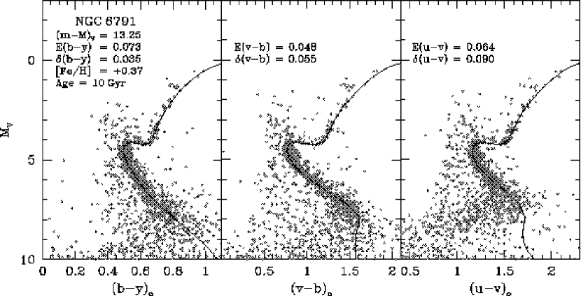
Figure 20: Strömgren CMDs for the metal rich open cluster NGC 6791 fitted with a 10 Gyr, $\rm{[Fe/H]}=+0.37$ isochrone. The indicated values of reddening, distance, and age are the same as those adopted in Paper I from fits to cluster data on the $B-V$ and $V-I$ CMDs. Note the rather large color offsets required to properly fit the cluster turnoff in each panel can be most likely attributed to uncertainties in the zero-points of our $uvby$ photometry (see the text).

As a final test of colors at $\rm{[Fe/H]}>0.0$ we present $uvby$ CMDs of the metal-rich open cluster NGC 6791 overlaid with our best fit 10 Gyr, $\rm{[Fe/H]}=+0.37$ isochrone. Since the metallicity of this cluster lies much closer to our set of colors at $\rm{[Fe/H]}=+0.5$ than the Hyades, its photometry can be used as a somewhat more stringent test of the color-temperature relations at such high metal abundances. The estimates for the cluster distance and reddening indicated in Figure 20 are the same as the values assumed in Paper I from the fits of the same 10 Gyr isochrone to the $B-V$ and $V-I$ CMDs. As mentioned in Paper I, these estimates may not necessarily be the correct ones given that other authors have quoted somewhat lower $\rm{[Fe/H]}$ and age values by about 0.2 dex and 2 Gyr, respectively. Unfortunately, our interpretation of the data is consistent with Paper I only if rather large color shifts are applied to the isochrone in all three CMDs. In this regard we note that our $uvby$ data for NGC 6791 is somewhat preliminary, and they appear to suffer from uncertainties in the zero-points for the calibrated photometry. Indeed, we have found that there is a 0.04 mag difference between our Strömgren $y$ magnitudes and the Johnson $V$ magnitudes published by Stetson, Bruntt, & Grundahl (2003). Since their broadband photometry has been standardized with extreme care and exhibits good consistency with other data sets, we are inclined to conclude that the $uvby$ data presented here are in error, at least with regards to the photometric zero-points. However, we are unable to say if there are also zero-point errors in the other three Strömgren filters, and therefore, we do not know to what extent the colors are affected by such errors. More observations are needed to shed light on this problem and to check the reliability of our color transformations for stars having higher metallicities than that of the Hyades.

3.5 Population II Subdwarfs

To further assess the accuracy of the calibrated colors for sub-solar metallicities, we have selected a number of Population II subdwarfs from Table 3 that are among the most well-studied metal-deficient field stars in the literature. The goal of this particular analysis is to check whether we can correctly reproduce the observed Strömgren colors for these subdwarfs provided accurate estimates of their parameters are available.

Since the $b-y$ index is highly sensitive to $T_{\rm{eff}}$, we first ensure that the IRFM temperatures for our sample of subdwarfs are consistent with those from other studies. Table 5 presents such a comparison for temperatures extracted from a number of different sources. The second column lists the mean of those temperatures quoted in the studies of Gratton et al. (1996; 2000) and/or Clementini et al. (1999). Each of these studies rely upon either empirical or theoretical color-temperature relationships to derive $T_{\rm{eff}}$. The effective temperatures presented by Axer, Fuhrmann, & Gehren (1994) and Fuhrmann (1998) were computed by fitting theoretical spectra to Balmer line profiles, and Allende Prieto & Lambert (2000) derived $T_{\rm{eff}}$ by analyzing the flux distribution in the near-UV continuum.

Although all of these studies rely upon different methods of deriving $T_{\rm{eff}}$, they appear to yield quite consistent results. In general, most of the IRFM temperatures show good agreement with those taken from the indicated studies to within $\pm 100\,$K, the most notable case being HD 19445, for which the temperature estimates lie within 25 K of each other. The two subdwarfs HD 134439 and HD 134440, however, both have IRFM temperatures that are $\approx$100$-$150 K cooler than those derived from the other studies. While the reasons for the differences in $T_{\rm{eff}}$ are not immediately apparent, we will assess the implications for the $uvby$ colors of adopting slightly warmer temperatures for these two stars.

In order to calculate the Strömgren colors for our subdwarfs, accurate estimates of the surface gravities and metallicities must supplement the IRFM temperatures for these stars. As mentioned earlier, the mean spectroscopic values for $\rm{log~{}g}$ and $\rm{[Fe/H]}$ from the catalog of Cayrel de Strobel et al. (2001) are favored over those included in the original AAM96 list from which these subdwarfs were extracted. In Table 6 we present the adopted stellar parameters together with the dereddened $uvby$ and $B-V$ photometry for the sample of subdwarfs. Furthermore, since all of these subdwarfs have very accurate parallaxes from Hipparcos, the $\rm{log~{}g}$ estimates derived from isochrones of Bergbusch & VandenBerg (2001), assuming the spectroscopic $\rm{[Fe/H]}$ values, have also been included for comparison. Table 6 also lists, again for comparison, the photometric $\rm{[Fe/H]}$ estimates derived from Strömgren metallicity calibrations by Schuster & Nissen (1989b). Finally, the Strömgren photometry for these subdwarfs are taken from the study of Schuster & Nissen (1988) and corrected for reddening using the $\rm{E{\it(B-V)}}$ values from Carretta et al. (2000). It is important to note that the subdwarf photometry is on the original Strömgren system, and so the comparisons which follow do not suffer from possible uncertainties in the transformation from the CCD system to the original system.

In Table 7 we list the results of numerous calculations carried out in an attempt to match the observed colors of the subdwarfs. The Strömgren indices are calculated from direct interpolation in the grid of calibrated colors, while the $B-V$ colors are derived from the broadband color transformations of Paper I. For all of the subdwarfs listed in the table, the first set of colors (Model A) is based on the stellar parameters presented in Table 6 (i.e., the IRFM temperatures, together with the spectroscopic values of $\rm{log~{}g}$ and $\rm{[Fe/H]}$). In addition, for a few selected subdwarfs (HD 19445, HD 103095, HD 140283, and HD 201891) we investigate the effects that uncertainties in the stellar parameters have on the computed photometry.

The majority of subdwarfs in Table 7 show excellent agreement between the observed and computed indices for the first set of parameters, considering that the observed colors have uncertainties of $\sim 0.01$ mag due to errors in the observations and transformation to the standard system. The other calculations that are listed confirm that the $b-y$ colors is indeed most sensitive to uncertainties in $T_{\rm{eff}}$, while the $m_{1}$ and $c_{1}$ indices are largely dependent on the accuracy of the adopted $\rm{[Fe/H]}$ and $\rm{log~{}g}$ values, respectively.

However, a few halo stars show some disagreement between their observed and computed colors. The most notable case is HD 25329, which has a difference of almost 0.06 mag in the $m_{1}$ index. It seems highly unlikely that errors in the adopted $T_{\rm{eff}}$ for this star could cause such a mismatch given the consistency of both the $T_{\rm{eff}}$ estimates (see Table 5) and the calculated and observed $b-y$ and $B-V$ colors. It is also unlikely that the star could have a surface gravity or metallicity that deviates significantly from the parameters listed in Table 6. Moreover, even if the reddening is non-zero, as we have assumed, this would only serve to $increase$ the dereddened value of $m_{1}$ [since $m_{o}=m_{1}+0.24\rm{E{\it(B-V)}}$]. Finally, we also note that Olsen (1993) obtains $uvby$ colors for HD 25329 ($b-y=0.525$, $m_{1}=0.305$, and $c_{1}=0.130$), which are in excellent agreement with those presented in Table 7.

Thus, we are left to conclude that the discrepancies are due to chemical abundance anomalies in the star’s atmosphere. It is known that HD 25329 exhibits unusually strong CN absorption features for its classification as a metal-poor halo star (Spiesman, 1992), and a few recent studies have shown that variations in the abundances of carbon and nitrogen can affect the Strömgren $m_{1}$ and $c_{1}$ indices (Grundahl et al., 2002a; Hilker, 2000). Specifically, the Strömgren $v$ filter is centered almost exactly on the CN band located at 4215Å while the NH molecular band sits within the $u$ filter at 3360Å. Therefore, we should expect any star with abnormal abundances of carbon and nitrogen to have somewhat different $m_{1}$ and $c_{1}$ values than one with “normal” abundances. This motivates us to try to find a CN-enhanced model that is better able to reproduce the observed indices of HD 25329, on the assumption of the same stellar parameters as before (4842/4.66/$-$1.65). The first such model (Model B) assumes that [C/Fe] = [N/Fe] = +0.4, while models C and D assume that carbon and nitrogen have been enhanced, in turn, by this amount. It appears that when both carbon and nitrogen are enhanced by +0.4 dex, the resulting colors show the best agreement with their observed counterparts. In support of this result, we note that Carbon et al. (1987) derived abundances of [C/Fe] = +0.44 and [N/Fe] = +0.45 for HD 25329 based on high-resolution spectroscopy.

For the few other subdwarfs whose calculated and observed colors differ, we include additional models in which the values for $T_{\rm{eff}}$ and/or $\rm{[Fe/H]}$ have been slightly altered to produce better agreement. For example, the second model for HD 140283 adopts the $T_{\rm{eff}}$ listed in column 3 of Table 5, which is $\sim 120\,$K higher than that obtained from the IRFM. Clearly, this particular model yields much better agreement for the $b-y$ and $B-V$ indices. A somewhat higher temperature was also obtained by Gratton, Carretta, & Castelli (1996) and Fuhrmann (1998). Such an increase in temperature is justified by the fact that HD 140283 likely has a non-negligible reddening (Grundahl et al., 2000a), which was not taken into account by AAM96. Finally, for the subdwarf pair HD 134439 and HD 134440, Model B adopts temperatures listed in column 2 of Table 5. While these somewhat higher temperatures improve the agreement for the $b-y$ index, an additional model (Model C) that assumes the photometric metallicities listed in column 5 of Table 6 yields the best overall agreement in all three Strömgren colors. In support of these new models, we note that Clementini et al. (1999) derived $\rm{[Fe/H]}=-1.30$ for HD 134439 and $\rm{[Fe/H]}=-1.28$ for HD 134440.

In conclusion, our calibrated Strömgren colors appear to provide a satisfactory match to the observed photometry for most of the “classical” subdwarfs. Although a few of the stars exhibit some discrepancies between their calculated and observed colors, we have shown that these can be largely explained by slightly altering their basic parameters within justifiable limits.

4 Previous Strömgren Color–T_eff Relations and Calibrations

Since our semi-empirically corrected $uvby$ transformations appear to be reliable in the variety of tests presented so far, we now compare them with other $uvby$ color–$T_{\rm{eff}}$ relations and calibrations that are available in the literature. In addition, we investigate if our colors can reproduce the loci of constant $\rm{[Fe/H]}$ in ($b-y$, $m_{1}$) space that are predicted by the Strömgren metallicity calibrations of Schuster & Nissen (1989a) for dwarfs and Hilker (2000) for giants.

4.1 Comparisons with Other Synthetic Strömgren Color–T_eff Relations

The grids of synthetic Strömgren colors considered for our comparison are those derived from the previous MARCS/SSG models of VandenBerg & Bell (1985, hereafter VB85) as well as latest set from CGK97 computed from Kurucz model atmospheres without overshooting. It is important to note, however, that both VB85 and CGK97 adopted the same $uvby$ filter transmission functions (Crawford & Barnes, 1970b) and use Vega as their zero-point standard. Therefore, any differences between the synthetic grids from these studies can largely be attributed to differences in the MARCS/SSG and ATLAS9 codes.

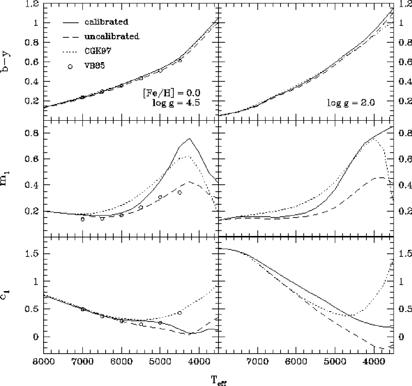
Figure 22: Same as Fig. 21 but for $\rm{[Fe/H]}=0.0$.

The CGK97 study provides the optimal set of colors against which we will compare our calibrated (and uncalibrated) color–$T_{\rm{eff}}$ relations due to fact that their coverage of parameter space for cool stars (i.e., $T_{\rm{eff}}<8000\,$K) is comparable to our own. While comparisons between our uncalibrated MARCS/SSG colors and those of VB85 are useful in investigating improvements in these models over the years, the colors computed by the latter cover a much more limited range in temperature and gravity. In Figures 21 and 22 we compare our calibrated and uncalibrated colors to those of CGK97 and VB85 for two representative metallicities of $\rm{[Fe/H]}=-1.5$ and 0.0 and gravities of $\rm{log~{}g}=4.5$ (dwarfs) and 2.0 (giants). At first glance, there are only very small differences between the VB85 and $uncalibrated$ dwarf $b-y$ colors in both metallicity cases. In addition, there is decent correspondence between the dwarf $m_{1}$ and $c_{1}$ indices of VB85 and our purely synthetic ones for temperatures in the range of 5500$-$7000 K. For temperatures below 5500 K, however, these VB85 indices start to deviate systematically from their $uncalibrated$ counterparts. These differences are largely due to advancements in the MARCS/SSG modeling routines over the years, such as the inclusion of more detailed atomic and molecular line lists and improved low-temperatures opacities since the VB85 colors were calculated.

Turning to the ATLAS9 color grids, the $b-y$ indices of CGK97 tend to show better agreement with the $calibrated$ colors for both metallicity cases. However, there are some significant discrepancies in $m_{1}$ at temperatures between 4500 and 7000 K — the $m_{1}$ indices of CGK97 tend to be systematically redder than our calibrated colors by up to 0.1 mag. within the temperature range encompassing late-F through early-K type dwarfs and giants. For models cooler than $\sim 4500\,$K, the CGK97 colors shift to being systematically too blue for the dwarfs. Moreover, fairly large discrepancies between our $c_{1}$ colors and those of CGK97 are also quite obvious in the metallicity and gravity regimes considered here.

These large discrepancies between our colors and those of CGK97 are most likely due to differences in the absorption line lists that are used to compute the synthetic spectra. BPT94 noted that the lines lists of Kurucz include a number of predicted absorption lines in the spectral regions of the Strömgren $v$ and $u$ filters that are not observed in the solar spectrum. Such an overestimate in line absorption would ultimately lead to fainter magnitudes in these passbands (hence larger values for $m_{1}$ and $c_{1}$) than what are actually observed, especially for cooler and/or more metal-rich models owing to the increased strength of metallic features towards later spectral types and higher metallicities.

To further exemplify the consequences of differences in the theoretical $uvby$ transformations considered here, Figure 23 plots two different isochrones corresponding to the indicated ages and metallicities that have been transformed to the various Strömgren color-magnitude planes using the current color transformations (both uncalibrated and calibrated) as well as those of CGK97. We note that identical bolometric corrections (namely those from Paper I) have been used to derive the $M_{V}$ values in each CMD to ensure that any differences between the isochrones are due solely to the color transformations. While it is encouraging that the calibrated and CGK97 $b-y$ isochrones agree quite well, there are fairly large differences between the $v-b$ and $u-v$ isochrones. As found in Paper I concerning the $(B-V)$–$T_{\rm{eff}}$ relations, the $uvby$ transformations of CGK97 will not provide as good a match of the 4 Gyr isochrone to the M 67 CMDs as those presented in this study.

4.2 Comparisons with Empirical (b – y)–T_eff Relations

There are several empirical calibrations of $b-y$ versus $T_{\rm{eff}}$ that have been widely used in recent years:

• Saxner & Hammärback (1985, hereafter SH85) presented one of the first empirical calibrations of $b-y$ vs. $T_{\rm{eff}}$ based on stellar temperatures derived using the IRFM. Their examination was based on a total of 30 dwarf stars ranging in temperature between 5800 and 7000 K whose colors fall within the range of $0.20<b-y<0.40$. While the stars used in their study covered a limited range in metallicity, an abundance term was included in the final calibration to account for the dependence on $\rm{[Fe/H]}$.

• The IRFM temperatures for $\sim 75$ stars used in the Gratton, Carretta, & Castelli (1996, hereafter GCC96) calibration were collected from the lists of BG89 and corrected to the same temperature scale as Blackwell & Lynas-Gray (1994). This large sample of stars covered a much wider range in temperature than the aforementioned SH85 study, and the final GCC96 calibration can be reasonably applied to solar-metallicity dwarf stars with $0.06\leq\,b-y\,\leq 0.95$.

• The $(b-y)$–$T_{\rm{eff}}$ calibrations of Alonso, Arribas, & Martínez-Roger (1996b, hereafter AAM96b) for dwarfs makes use of the same IRFM temperatures that we have used to calibrate the synthetic $uvby$ colors in the present study. This sample is by far the largest to date with well-determined $T_{\rm{eff}}$’s, and it includes stars with spectral types between F0 and K5 covering a wide range in metallicity ($-3.0\leq\rm{[Fe/H]}\leq+0.5$). To account for the effects of differing metal abundances and gravity, their final dwarf-star calibration is given as a function of both $\rm{[Fe/H]}$ and $c_{1}$.

Figure 24 compares these three empirical $(b-y)$–$T_{\rm{eff}}$ calibrations together with the relationship predicted by our solar metallicity ZAMS model. For those calibrations that include a metallicity term (SH85 and AAM96b), $\rm{[Fe/H]}=0.0$ is assumed. Also since the AAM96b calibration includes a $c_{1}$ term, we opt to use the $c_{1}$ predictions from our ZAMS to plot their trend between $b-y$ and $T_{\rm{eff}}$. It is quite reassuring that all three empirical calibrations agree rather well in the range $0.2<b-y<0.6$, which illustrates the good consistency among the several studies that have used the IRFM to infer stellar temperatures. In addition, Figure 24 demonstrates that our calibrated Strömgren colors can accurately relate $b-y$ to temperature. Indeed, our ZAMS is in superb agreement (to well within $\pm 100\,$K) with the empirical relationships of GCC96 and AAM96b over a range in $b-y$ corresponding to F- and G-type stars.

4.3 Strömgren [Fe/H] Calibration for Dwarf Stars

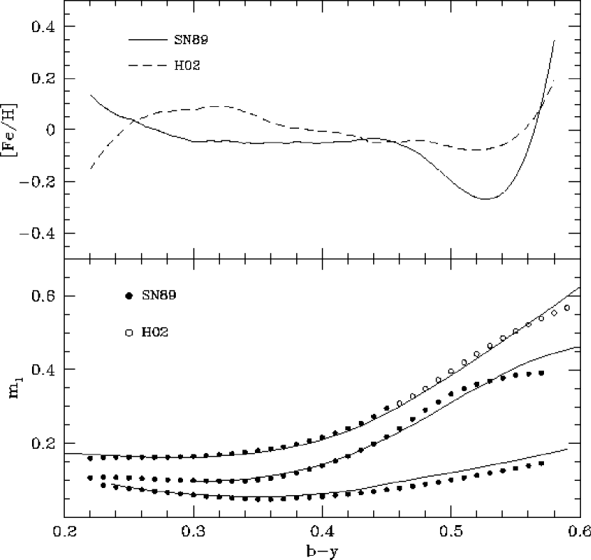
Figure 25: Top panel: The $\rm{[Fe/H]}$$-(b-y)$ relations computed from the Schuster & Nissen (1989a) and Haywood (2002) Strömgren metallicity calibrations using the colors from our solar metallicity ZAMS model. Note the large discrepancy in the SN89 calibration for $b-y\gtrsim 0.47$. Bottom panel: The $b-y$ and $m_{1}$ predictions from SN89 and H02 calibrations are compared with our ZAMS models for $\rm{[Fe/H]}=0.0$, $-1.0$, and $-2.0$.

The Strömgren $\rm{[Fe/H]}$ calibrations of Schuster & Nissen (1989a, hereafter SN89) have served as an efficient way to determine the photometric metallicities of F- and G-type dwarf stars, and they have been widely used in the past to investigate the metallicity distributions of field stars in the Galactic disk and halo. The SN89 relationships were derived from a sample of Population I and II stars having $\rm{[Fe/H]}$ estimates from high-dispersion spectroscopy and employed the standard $uvby$ indices rather than relying on the differential indices, $\delta$$m_{1}=m_{1}^{Hyades}-m_{1}^{star}$ and $\delta$$c_{1}=c_{1}^{Hyades}-c_{1}^{star}$, used in previous Strömgren metallicity calibrations (e.g., the relations of Crawford, 1975; Olsen, 1984). To further investigate the quality of our corrected transformations at $\rm{[Fe/H]}=0.0$, we have employed the colors of our solar metallicity ZAMS model to derive $\rm{[Fe/H]}$ values as a function of $b-y$ using the analytic formulae given by SN89. As shown in the top panel of Figure 25, the resultant relationship tends to hold constant at a value of $\rm{[Fe/H]}\approx-0.05$ at $0.3\lesssim\,b-y\,\lesssim 0.45$, but it deviates towards lower metallicity values at $0.46\lesssim\,b-y\,\lesssim 0.52$ and towards higher values at $b-y\gtrsim 0.53$. (Note that we would obtain a horizontal line at $\rm{[Fe/H]}=0.0$ if our respective calibrations were identical.) From this evidence one could conclude that our colors for cooler stars are in error. However, given the rather good agreement between our ZAMS model and the Hipparcos data (and empirical standard relations) presented in Section 3.3, we are reluctant to make any changes to the transformations at $\rm{[Fe/H]}=0.0$ that would correct the discrepancies in Figure 25.

We do note that a similar trend in the photometric $\rm{[Fe/H]}$ values for solar neighborhood F- and G-type dwarf stars computed using the SN89 calibrations has also been discovered recently by Twarog, Anthony-Twarog, & Tanner (2002) and Haywood (2002, hereafter H02). Both of these studies employ a sample of stars from the Hyades as well as nearby Hipparcos field stars to illustrate that their computed $\rm{[Fe/H]}$ values from SN89 are systematically underestimated by 0.1 to 0.4 dex in the color range corresponding to mid- to late-G dwarfs. While the Twarog study argues that the $c_{1}$ index for cooler dwarf stars is strongly affected by variations in $\rm{[Fe/H]}$, H02 concludes there is no obvious additional dependence of the SN89 calibrations on $c_{1}$: the latter rederives the coefficients in the SN89 metallicity calibrations. In the top panel of Figure 25 we also plot the relationship between $b-y$ and the $\rm{[Fe/H]}$ values derived using the new H02 calibrations (dashed line). Although we would argue that the H02 relationship tends to slightly overestimate $\rm{[Fe/H]}$ values for stars with $0.26\lesssim\,b-y\,\lesssim 0.40$ and slightly underestimate them at $0.40\lesssim\,b-y\,\lesssim 0.56$, much of the discrepancy at $b-y\gtrsim 0.47$ has been removed. In addition, the fact that the computed H02 $\rm{[Fe/H]}$ values are within $\pm 0.1$ dex of $\rm{[Fe/H]}=0.0$ across wide range in $b-y$ is quite reassuring since the photometric metallicity estimates derived from these calibrations are expected to be uncertain by at least this amount.

In the bottom panel of Figure 25, we compare the relationship between $b-y$ and $m_{1}$ given by the SN89 calibrations (filled circles) to our ZAMS predictions for $\rm{[Fe/H]}$ values of 0.0, $-1.0$, and $-2.0$. Since the SN89 calibrations are known to underestimate $\rm{[Fe/H]}$ for metallicities near solar and $b-y\geq 0.450$ (as discussed above), we have elected to plot the late-G dwarf calibration of H02 (open circles, their Eq. 4) for $b-y$ colors redder than this value. Clearly, the agreement between our ZAMS models and the calibrations of SN89 and H02 is quite satisfactory.

4.4 Strömgren [Fe/H] Calibration for Giant Stars

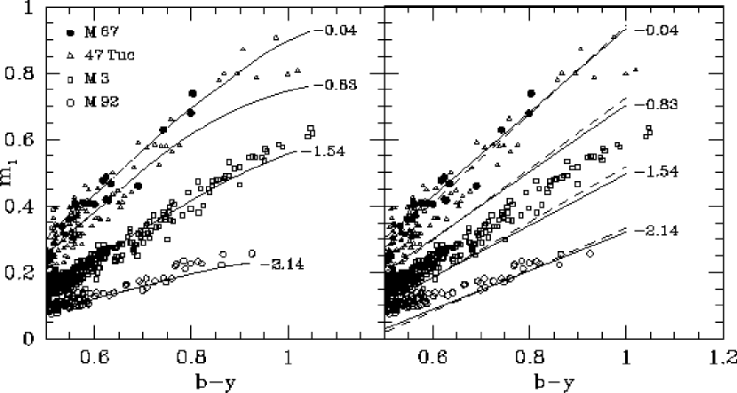
Figure 26: The location of RGB stars from the clusters M 92, M 3, 47 Tuc, and M 67 in ($b-y$, $m_{1}$) space. The solid lines in the left-hand panel denote the giant branch predictions from the same isochrones used to fit these clusters in the preceding sections. The solid and dashed lines in the right panel are the two giant star metallicity calibrations of Hilker (2000) plotted for the indicated $\rm{[Fe/H]}$ values.

In Figure 26 we plot on the ($b-y$, $m_{1}$) plane the locations of RGB stars from some of the clusters that have been considered in this study. The cluster photometry has been corrected for reddening using the same values (derived from the reddening maps of Schlegel et al.) denoted in the previous figures. With the exception of 47 Tuc, the RGB stars from each cluster generally follow a fairly tight and nearly linear relationship between their $b-y$ and $m_{1}$ colors. The increased scatter seen in the RGB of 47 Tuc can likely be explained by the presence of star-to-star differences in the amount of CN absorption. Variations in the strength of CN bands among stars in 47 Tuc were first observed by Norris & Freeman (1979) and analyzed for abundances by Dickens, Bell, & Gustafsson (1979). Similar variations in main-sequence stars were first found by Hesser (1978) and have been analyzed by several authors including Hesser & Bell (1980). More recent work has been carried out by several authors including Briley (1997), Cannon et al. (1998), and Harbeck, Smith, & Grebel (2003). In terms of the $uvby$ photometry presented in Figure 26, those RGB stars with strong or weak CN features will manifest themselves as a scatter in the $m_{1}$ colors due to the location of a prominent CN absorption band within the Strömgren $v$ filter. Therefore, stars with abnormally large CN absorption will be scattered to large $m_{1}$ values while those with relatively weak CN bands will lie at smaller $m_{1}$.

In the left-hand panel of Figure 26, we overlay the RGB colors from the same isochrones that were used in the previous sections to fit the cluster data. Upon inspection of this plot it appears that our RGB models do a good job in reproducing not only the locations, but also the slopes of the observed giant branches for M 92, M 3, and M 67. In the case of 47 Tuc, however, it seems that our adopted isochrone lies on the blue side of the RGB distribution in $m_{1}$, especially for stars with $b-y\gtrsim 0.8$. As mentioned in the paragraph above, the fairly large scatter in the cluster photometry can likely be associated with stars having various amounts of CN absorption in their spectra. While we have no data at the moment that would help differentiate the 47 Tuc stars in Figure 26 according to their CN band strength, it suffices to say here that our $\rm{[Fe/H]}=-0.83$ RGB model most likely matches the locus of stars with weak CN absorption.

The right-hand panel of Figure 26 plots the same data for each cluster but overlaid with lines of constant $\rm{[Fe/H]}$ predicted from the red-giant metallicity calibrations of Hilker (2000). In this diagram we see that the two calibrations presented by Hilker, one based on 4 coefficients (solid line, their Eq. 1) and the other using 5 coefficients (dashed line, their Eq. 3), tend to overestimate the abundances of some globular clusters (by as much as 0.5 dex in the case of M 3 and 47 Tuc). The only case of good agreement with our results is for M 67 where both Hilker calibration lines fit the data nicely, and they correspond well with our RGB predictions (left-hand panel). In his derivation of the red-giant calibrations, Hilker employed a sample of RGB stars both from globular clusters (M 22, M 55, and $\omega\,$Cen) as well as from the field that had Strömgren photometry and spectroscopic metallicity estimates. While they claim to have placed their metallicities on the same scale as Zinn & West, Figure 26 does not support this as, for example, M 3 has $\rm{[Fe/H]}\approx-1.6$ on this scale. It is possible that the reddening values Hilker adopted for the globular clusters are in error: an overestimate in E$(B-V)$ of 0.05 mag translates approximately to a change in $\rm{[Fe/H]}$ by +0.25 dex, according to the Hilker calibrations. Therefore, the adoption of the correct reddening is a critical factor in determining the location of the iso-metallicity lines based on the cluster photometry. (However, since Hilker also used a number of nearby field giant stars with known metallicities, uncertainties in their reddening estimates of this magnitude is hardly possible.)

5 Summary & Conclusions

In this investigation, we have produced an extensive set of color-temperature relations for the Strömgren $uvby$ system that covers a broad range in $T_{\rm{eff}}$, $\rm{log~{}g}$, and $\rm{[Fe/H]}$. To be specific, at each $\rm{[Fe/H]}$ value in the range from $-3.0$ to $+0.5$, in steps of 0.5 dex, $b-y$, $m_{1}$, and $c_{1}$ colors are provided at $-0.5\leq\rm{log~{}g}\leq 5.0$ and $3000\leq T_{\rm{eff}}\leq 6000\,$K (in a “low-temperature” table), as well as at $2.0\leq\rm{log~{}g}\leq 5.0$ and $6000<T_{\rm{eff}}\leq 40,000\,$K (in a “high-temperature” table). The $v-b$ and $u-v$ colors are readily obtained from $m_{1}=(v-b)-(b-y)$ and $c_{1}=(u-v)-(v-b)$. By convention, Strömgren $y$ and Johnson $V$ magnitudes are similarly normalized, with the result that the bolometric corrections to $y$ are nearly identical with those to $V$ and typically differ by $\lesssim\,$0.01$-$0.02 mag over most of parameter space. As it is generally the case that observed $y$ magnitudes are calibrated to be on the $V$ magnitude scale, the $BC_{V}$ values reported in Paper I have been included in our color transformation tables in order for these tables and associated interpolation software to be a self-contained package.

The main thrust of this study has been to determine what corrections to purely synthetic color–$T_{\rm{eff}}$ relations are needed to ensure that the latter do the best possible job of satisfying empirical constraints. The starting point for our analysis consisted of a set of synthetic colors that were computed from MARCS model atmospheres and SSG synthetic spectra at $T_{\rm{eff}}\leq 8000\,$K, to which we appended the predictions for hotter stars as derived by Castelli, Gratton, & Kurucz (1997) from Kurucz non-overshooting model atmospheres. There were no obvious problems with this composite grid (in conjunction with modern isochrones) to reproduce Strömgren observations for extremely metal-poor turnoff and giant stars (those having $\rm{[Fe/H]}\lesssim-2.0$), as in the globular cluster M 92. Indeed, a completely consistent interpretation of the cluster data was found regardless of which color plane was examined, and that interpretation was virtually identical to that obtained from a consideration of $BV$ data in Paper I. Discrepancies between theory and observations became evident for cool dwarfs with $\rm{[Fe/H]}\approx-2.0$ via our comparisons to a sample of extremely metal-poor field stars. Moreover, as the metallicity increased, the predicted $uvby$ colors tended to be systematically bluer than observed ones. We assume that at least part of these discrepancies, particularly in the Strömgren $u$ and $v$ filters, can be attributed to incomplete atomic and molecular line lists, not incorporating the Fe I continuous opacity source (Bell, Balachandran, & Bautista, 2001) in the SSG computations, and neglecting CN processing in the atmospheres of our giant star models. It is important to note, however, that the neglect of such CN variations in giants (or the improved treatment of Fe I continuous opacity) is not a concern for the calibrated color–$T_{\rm{eff}}$ relations that are presented in this paper because our transformations have been constrained to reproduce the colors of observed stars.

We first corrected the synthetic colors for $\rm{[Fe/H]}=0.0$ using a fairly large sample of solar metallicity field stars having accurate $T_{\rm{eff}}$ determinations from the infrared flux method. These adjustments tended to be rather large for cool stars, but they were nonetheless necessary to place the colors on the same system as the photometric data. Important confirmation of the accuracy of the corrected transformations was provided by fitting isochrones to the CMD of the open cluster M 67 where models for the observed metallicity, and whose $T_{\rm{eff}}$ scale was precisely normalized to the Sun, yielded a superb match to the observations. [As cluster data played a only limited role in the derivation of the color adjustments, and as the same interpretation of the data was obtained here as in Paper I, which analyzed $BV(RI)_{C}$ observations, we conclude that our transformations are accurate and fully consistent with those reported in Paper I for the Johnson-Cousins photometric systems.]

We found that the necessary adjustments to the synthetic colors at $T_{\rm{eff}}>5500\,$K or $\rm{log~{}g}<3.5$ varied nearly linearly with $\rm{[Fe/H]}$, whereas those outside this regime were constrained based on a sample of cool field and cluster dwarf stars. Indeed, upon applying these corrections at $-1.5\leq\rm{[Fe/H]}\leq-0.5$ and $\rm{[Fe/H]}=+0.5$, it was possible to achieve very good fits of isochrones to the CMDs of M 3 and 47 Tuc, which have $\rm{[Fe/H]}\approx-1.55$ and $-0.75$, respectively, as well as to that of the Hyades ($\rm{[Fe/H]}=0.12$). Once again, there was excellent consistency with the results reported in Paper I concerning the $BV(RI)_{C}$ system. Only at higher metal abundances did inconsistencies arise as demonstrated by the fact that our fit of the same isochrones used in Paper I to the CMD of the $\rm{[Fe/H]}\approx\,+0.4$ open cluster NGC 6791 required a significant color offset to match the photometry if the same reddening used in Paper I was adopted. As we have been unable to understand this discrepancy, which may require further observations to resolve it, our transformations at $\rm{[Fe/H]}\gtrsim 0.15$ (probably those in Paper I as well) should be used with caution. More observational constraints are needed to put the color–$T_{\rm eff}$ relations for super-metal-rich stars on a firm foundation.

We have found good consistency between our $(b-y)$–$T_{\rm{eff}}$ relation for dwarf stars having near solar abundances and those derived by Saxner & Hammärback (1985), Gratton et al. (1996), and Alonso et al. (1996b). Comparisons between the predicted and observed colors for the classic Population II subdwarfs have also offered encouraging support for our results. Moreover, the dependence of $m_{1}$ on $b-y$ predicted from our color transformations agrees well with the relations for solar-metallicity dwarfs derived by Schuster & Nissen (1989a) at $b-y\lesssim 0.45$ and by Haywood (2002) at redder colors, and with the relations for giants as inferred from a sample RGB stars from a number of globular and open clusters that encompass a wide range in $\rm{[Fe/H]}$.

It is our intention to update the transformations reported in this paper as new constraints become available. Even at this stage, however, we believe that our results represent a considerable improvement over currently available color–$T_{\rm{eff}}$ relations for the Strömgren photometric system and that their use will lead to important refinements in our our understanding of stars and stellar populations. The next paper in this series (Clem, VandenBerg, & Stetson, in preparation) will present color transformations for the Sloan $u^{\prime}g^{\prime}r^{\prime}i^{\prime}z^{\prime}$ system.

Table 1: Comparison of $T_{\rm{eff}}$ and $F_{\rm{bol}}$ Estimates

HR #	Spec. Type	AAM96/AAM99		BG89		SH85
		$F_{\rm{bol}}$	$T_{\rm{eff}}$	$F_{\rm{bol}}$	$T_{\rm{eff}}$	$F_{\rm{bol}}$	$T_{\rm{eff}}$
219…..	G0 V	113.80	5817	119.30	5839	-	-
434…..	K4 III	63.26	4046	68.40	4046	-	-
458…..	F8 V	60.34	6155	-	-	61.7	6154
464…..	K3 III	156.50	4359	167.30	4425	-	-
483…..	G1.5 V	27.88	5874	-	-	29.0	5856
617…..	K2 III	625.20	4490	652.00	4499	-	-
937…..	G0 V	63.74	5996	-	-	65.7	5994
1084…	K2 V	100.30	5076	109.30	5156	-	-
1101…	F9 IV-V	51.86	5998	-	-	52.0	5963
1325…	K1 V	53.11	5040	56.09	5114	-	-
1457…	K5 III	3247.00	3866	3422.00	3943	-	-
1543…	F6 V	137.40	6482	-	-	139.0	6373
1729…	G1.5 IV-V	35.09	5847	-	-	36.5	5819
1907…	K0 IIIb	81.93	4693	86.55	4719	-	-
1983…	F7 V	95.74	6260	-	-	97.6	6259
2085…	F1 V	83.01	7013	-	-	128.0	8144
2852…	F0 V	55.17	7020	-	-	55.1	6957
2943…	F5 IV-V	1844.00	6579	-	-	1860.0	6601
2990…	K0 IIIb	1140.00	4854	1236.00	4896	-	-
3323…	G5 III	135.50	5136	139.70	5176	-	-
4247…	K0 III	105.10	4643	112.40	4692	-	-
4496…	G8 V	20.99	5342	23.19	5552	-	-
4518…	K0.5 IIIb	135.50	4348	144.00	4421	-	-
4540…	F9 V	94.19	6095	-	-	100.0	6147
4785…	G0 V	53.19	5867	54.09	5861	54.3	5842
4883…	G0 IIIp	28.69	5589	30.50	5761	-	-
4932…	G8 III	225.10	5043	236.20	5052	-	-
4983…	F9.5 V	52.41	5964	55.09	6024	-	-
5340…	K1.5 III	4830.00	4233	5159.00	4321	-	-
5429…	K3 III	163.80	4271	175.30	4303	-	-
5447…	F2 V	43.28	6707	-	-	42.5	6696
5634…	F5 V	27.55	6571	-	-	28.0	6616
5681…	G8 III	134.20	4798	142.30	4832	-	-
5868…	G0 V	45.14	5897	-	-	46.7	5940
5914…	F8 Ve	39.00	5774	-	-	41.7	5802
5933…	F6 IV	75.90	6233	-	-	78.4	6246
6220…	G7.5 IIIb	126.10	4942	131.90	4913	-	-
6603…	K2 III	295.20	4533	310.80	4603	-	-
6705…	K5 III	805.80	3934	890.60	3955	-	-
6869…	K0 III-IV	165.80	4835	177.50	4949	-	-
7429…	K3 IIIb	65.39	4473	69.71	4456	-	-
7462…	K0 V	40.12	5227	42.49	5253	-	-
7503…	G1.5 Vb	11.15	5763	11.33	5826	-	-
7504…	G3 V	8.96	5767	9.31	5664	-	-
7615…	K0 III	93.60	4796	96.90	4887	-	-
7957…	K0 IV	136.60	4908	147.90	4996	-	-
8085…	K5 V	37.15	4323	39.43	4463	-	-
8086…	K7 V	22.20	3865	25.33	4252	-	-
8255…	K1 III	39.63	4609	43.30	4715	-	-
8832…	K3 V	20.44	4785	22.42	4896	-	-
8905…	F8 IV	46.12	5954	-	-	47.5	5897

Table 2: Comparison of Stellar Angular Diameters

HR #	$\theta_{BG89}$	$\theta_{AAM99}$	$\theta_{N99/N01}$	$\pi$ (mas)
163…..	-	1.72 $\pm$ 0.08	1.77 $\pm$ 0.08	19.34 $\pm$ 0.76
165…..	-	4.20 $\pm$ 0.22	4.24 $\pm$ 0.06	32.19 $\pm$ 0.68
168…..	-	5.66 $\pm$ 0.28	5.65 $\pm$ 0.08	14.27 $\pm$ 0.57
464…..	3.62 $\pm$ 0.19	3.61 $\pm$ 0.19	3.76 $\pm$ 0.07	18.76 $\pm$ 0.74
489…..	-	3.00 $\pm$ 0.16	2.81 $\pm$ 0.03	8.86 $\pm$ 0.77
617…..	6.91 $\pm$ 0.35	6.80 $\pm$ 0.35	6.94 $\pm$ 0.08	49.48 $\pm$ 0.99
824…..	1.99 $\pm$ 0.10	-	1.88 $\pm$ 0.11	18.06 $\pm$ 0.84
1409…	2.64 $\pm$ 0.13	-	2.41 $\pm$ 0.11	21.04 $\pm$ 0.82
2943…	5.42 $\pm$ 0.21	5.43 $\pm$ 0.21	5.43 $\pm$ 0.07	285.93 $\pm$ 0.88
2990…	8.04 $\pm$ 0.39	7.88 $\pm$ 0.38	7.95 $\pm$ 0.09	96.74 $\pm$ 0.87
3249…	5.17 $\pm$ 0.29	-	5.13 $\pm$ 0.04	11.23 $\pm$ 0.97
3547…	-	3.24 $\pm$ 0.16	3.29 $\pm$ 0.08	21.64 $\pm$ 0.99
3705…	-	7.33 $\pm$ 0.42	7.50 $\pm$ 0.09	14.69 $\pm$ 0.81
3873…	2.72 $\pm$ 0.12	-	2.70 $\pm$ 0.10	13.01 $\pm$ 0.88
3980…	3.41 $\pm$ 0.19	-	3.33 $\pm$ 0.04	11.89 $\pm$ 0.72
4247…	2.64 $\pm$ 0.13	2.61 $\pm$ 0.13	2.54 $\pm$ 0.03	33.40 $\pm$ 0.78
4301…	6.79 $\pm$ 0.34	-	6.91 $\pm$ 0.08	26.38 $\pm$ 0.53
4335…	4.18 $\pm$ 0.21	-	4.08 $\pm$ 0.07	22.21 $\pm$ 0.68
4432…	-	3.23 $\pm$ 0.18	3.21 $\pm$ 0.03	5.40 $\pm$ 0.99
4518…	3.36 $\pm$ 0.17	3.37 $\pm$ 0.18	3.23 $\pm$ 0.02	16.64 $\pm$ 0.60
4932…	3.30 $\pm$ 0.15	3.23 $\pm$ 0.15	3.23 $\pm$ 0.05	31.90 $\pm$ 0.87
5253…	2.26 $\pm$ 0.09	-	2.28 $\pm$ 0.07	13.01 $\pm$ 0.63
5602…	2.61 $\pm$ 0.12	-	2.48 $\pm$ 0.08	14.91 $\pm$ 0.57
5681…	2.80 $\pm$ 0.14	2.76 $\pm$ 0.13	2.76 $\pm$ 0.03	27.94 $\pm$ 0.61
5854…	4.96 $\pm$ 0.25	-	4.83 $\pm$ 0.09	44.54 $\pm$ 0.71
6220…	2.61 $\pm$ 0.12	2.52 $\pm$ 0.12	2.50 $\pm$ 0.08	29.11 $\pm$ 0.52
6418…	5.52 $\pm$ 0.30	-	5.26 $\pm$ 0.06	8.89 $\pm$ 0.52
7314…	2.40 $\pm$ 0.12	-	2.23 $\pm$ 0.09	4.24 $\pm$ 0.49
7328…	-	2.22 $\pm$ 0.11	2.07 $\pm$ 0.07	26.48 $\pm$ 0.49
7602…	2.16 $\pm$ 0.10	-	2.18 $\pm$ 0.09	72.95 $\pm$ 0.83
7957…	2.67 $\pm$ 0.13	2.66 $\pm$ 0.13	2.65 $\pm$ 0.04	69.73 $\pm$ 0.49
8632…	-	2.62 $\pm$ 0.14	2.63 $\pm$ 0.05	10.81 $\pm$ 0.56
8684…	2.47 $\pm$ 0.12	-	2.53 $\pm$ 0.09	27.95 $\pm$ 0.77
8923…	-	1.53 $\pm$ 0.07	1.61 $\pm$ 0.17	18.34 $\pm$ 0.74
8961…	-	2.73 $\pm$ 0.14	2.66 $\pm$ 0.08	38.74 $\pm$ 0.68

Table 3: Field Star Sample

Hip. ID	$T_{\rm{eff}}$	$\rm{log~{}g}$	$\rm{[Fe/H]}$	V	$(B-V)$	E$(B-V)$	$(b-y)$	$m_{1}$	$c_{1}$	Source
80	5859	4.24	-0.59	8.40	0.566	0.000	0.372	0.143	0.309	2
434	5351	2.66	-1.45	9.04	0.692	0.008	0.434	0.092	0.474	3
484	4968	2.60	-1.10	9.66	0.787	0.000	0.513	0.155	0.349	3
910	6148	4.11	-0.35	4.89	0.487	0.003	0.328	0.130	0.405	1
1298	5265	2.60	-1.10	9.58	0.710	0.015	0.460	0.129	0.464	3
1301	5784	4.15	-0.85	9.74	0.569	0.000	0.383	0.135	0.284	2

Table 4: Coefficients for the Calibrations Between Synthetic and Observed Color

Color	A	B	C	N	$\sigma$	Range
$(b-y)$….
dwarfs	0.003$\,\pm\,$0.006	1.077$\,\pm\,$0.011	-	102	0.020	$0.15\leq\,b-y\,\leq 0.78$
giants	0.004$\,\pm\,$0.007	1.084$\,\pm\,$0.012	-	61	0.025	$0.15\leq\,b-y\,\leq 0.82$
dwarfs & giants	-0.001$\,\pm\,$0.005	1.080$\,\pm\,$0.009	-	163	0.023	$0.15\leq\,b-y\,\leq 0.82$
$m_{1}$…..
dwarfs	0.028$\,\pm\,$0.006	0.346$\,\pm\,$0.071	3.573$\,\pm\,$0.173	102	0.047	$0.10\leq\,m_{1}\,\leq 0.40$
giants	-0.127$\,\pm\,$0.007	2.083$\,\pm\,$0.026	-	61	0.044	$0.10\leq\,m_{1}\,\leq 0.45$

Table 5: Various $T_{\rm{eff}}$ Estimates for Selected Population II Subdwarfs

HD #	$T_{\rm{eff,IRFM}}$	$T_{\rm{eff,CT}}$	$T_{\rm{eff,Balmer}}$	$T_{\rm{eff,UV}}$
19445…..	6050	6054	6040	6065
25329…..	4842	4845	-	4870
64090…..	5441	5506	5499	5456
74000…..	6224	6275	6211	-
84937…..	6330	6344	6353	6389
103095…	5029	5097	5110	5069
132475…	5788	5758	-	-
134439…	4974	5120	-	5110
134440…	4746	4879	-	-
140283…	5691	5763	5814	-
188510…	5564	5628	5500	5597
201891…	5909	5974	5797	5929

Table 6: Fundamental Parameters and Photometry for Selected Population II Subdwarfs.

HD #	$\rm{log~{}g}$	$\rm{log~{}g}$	$\rm{[Fe/H]}$	$\rm{[Fe/H]}$	$\rm{E{\it(B-V)}}$	$(B-V)_{o}$	$(b-y)_{o}$	$m_{o}$	$c_{o}$
19445…..	4.38	4.44	-1.99	-1.92	0.002	0.458	0.351	0.052	0.203
25329…..	4.66	4.68	-1.68	-1.63	0.000	0.864	0.533	0.307	0.131
64090…..	4.49	4.58	-1.65	-1.69	0.000	0.614	0.428	0.110	0.126
74000…..	4.18	4.08	-2.01	-1.69	0.000	0.431	0.311	0.067	0.295
84937…..	3.97	4.05	-2.09	-2.14	0.009	0.382	0.296	0.058	0.352
103095…	4.62	4.61	-1.30	-1.33	0.000	0.752	0.484	0.222	0.155
132475…	3.85	3.84	-1.52	-1.32	0.037	0.522	0.373	0.072	0.279
134439…	4.63	4.63	-1.41	-1.33	0.005	0.767	0.480	0.225	0.164
134440…	4.59	4.62	-1.43	-1.24	0.005	0.845	0.520	0.298	0.172
140283…	3.50	3.69	-2.40	-2.49	0.024	0.463	0.362	0.039	0.280
188510…	4.54	4.57	-1.53	-1.57	0.001	0.598	0.415	0.100	0.163
201891…	4.33	4.29	-0.97	-1.08	0.003	0.514	0.360	0.095	0.260

Table 7: The Computed $uvby$ (and $B-V$) Photometry for Population II Subdwarfs

HD #	$(b-y)_{o}$	$m_{o}$	$c_{o}$	$(B-V)_{o}$		Notes
19445…..	0.351	0.052	0.203	0.458		Intrinsic colors
	0.345	0.051	0.212	0.450		Model A = (6050/4.38/-1.99)
	$\mp$0.014	$\pm$0.002	$\pm$0.018	$\mp$0.020		Model A: $T_{\rm{eff}}\pm 100\,$K
	$\pm$0.005	$\pm$0.001	$\mp$0.030	$\pm$0.006		Model A: $\rm{log~{}g}\pm 0.25\,$dex
	$\mp$0.003	$\pm$0.008	$\pm$0.010	$\pm$0.008		Model A: $\rm{[Fe/H]}\pm 0.25\,$dex
25329…..	0.533	0.307	0.131	0.864		Intrinsic colors
	0.538	0.250	0.122	0.844		Model A = (4842/4.66/-1.68)
	0.540	0.298	0.124	0.844		Model B = Model A w/ [C/Fe]=[N/Fe]=+0.4
	0.540	0.297	0.100	0.844		Model C = Model A w/ [C/Fe]=+0.4
	0.538	0.251	0.148	0.844		Model D = Model A w/ [N/Fe]=+0.4
64090…..	0.428	0.110	0.126	0.614		Intrinsic colors
	0.431	0.119	0.154	0.625		Model A = (5441/4.49/-1.65)
74000…..	0.311	0.067	0.295	0.431		Intrinsic colors
	0.321	0.052	0.283	0.412		Model A = (6224/4.18/-2.01)
84937…..	0.296	0.058	0.352	0.382		Intrinsic colors
	0.306	0.054	0.355	0.387		Model A = (6330/3.97/-2.09)
103095…	0.484	0.222	0.155	0.752		Intrinsic colors
	0.493	0.256	0.149	0.780		Model A = (5029/4.62/-1.30)
	$\mp$0.016	$\mp$0.025	$\mp$0.003	$\mp$0.035		Model A: $T_{\rm{eff}}\pm 100\,$K
	$\pm$0.001	$\pm$0.007	$\mp$0.011	$\pm$0.009		Model A: $\rm{log~{}g}\pm 0.25\,$dex
	$\mp$0.007	$\pm$0.037	$\mp$0.003	$\pm$0.004		Model A: $\rm{[Fe/H]}\pm 0.25\,$dex
132475…	0.373	0.072	0.279	0.522		Intrinsic colors
	0.367	0.081	0.257	0.513		Model A = (5788/3.85/-1.52)
134439…	0.480	0.225	0.164	0.767		Intrinsic colors
	0.505	0.257	0.140	0.798		Model A = (4974/4.63/-1.41)
	0.480	0.217	0.145	0.748		Model B = (5120/4.63/-1.41)
	0.479	0.227	0.153	0.749		Model C = (5120/4.63/-1.33)
134440…	0.520	0.298	0.172	0.845		Intrinsic colors
	0.550	0.322	0.131	0.881		Model A = (4746/4.59/-1.43)
	0.523	0.279	0.137	0.830		Model B = (4879/4.59/-1.43)
	0.519	0.308	0.152	0.833		Model C = (4879/4.59/-1.24)
140283…	0.362	0.039	0.280	0.463		Intrinsic colors
	0.384	0.039	0.266	0.493		Model A = (5691/3.50/-2.40)
	0.365	0.038	0.294	0.467		Model B = (5814/3.50/-2.40)
	$\mp$0.015	$\pm$0.001	$\pm$0.025	$\mp$0.021		Model B: $T_{\rm{eff}}\pm 100\,$K
	$\pm$0.003	$\pm$0.001	$\mp$0.046	$\pm$0.006		Model B: $\rm{log~{}g}\pm 0.25\,$dex
	$\mp$0.001	$\pm$0.007	$\pm$0.007	$\pm$0.005		Model B: $\rm{[Fe/H]}\pm 0.25\,$dex
188510…	0.415	0.100	0.163	0.598		Intrinsic colors
	0.412	0.115	0.162	0.593		Model A = (5564/4.54/-1.53)
201891…	0.360	0.095	0.260	0.514		Intrinsic colors
	0.360	0.109	0.249	0.523		Model A = (5909/4.33/-0.97)
	$\mp$0.013	$\mp$0.006	$\pm$0.016	$\mp$0.025		Model A: $T_{\rm{eff}}\pm 100\,$K
	$\pm$0.002	$\pm$0.005	$\mp$0.032	$\pm$0.008		Model A: $\rm{log~{}g}\pm 0.25\,$dex
	$\pm$0.005	$\pm$0.016	$\pm$0.021	$\pm$0.015		Model A: $\rm{[Fe/H]}\pm 0.25\,$dex

Figure 23: A comparison of two isochrones having $\rm{[Fe/H]}\approx-1.5$ and 0.0 for ages of 13 and 4 Gyr, respectively, which have been transformed to the various $uvby$ CMDs using the theoretical Strömgren colors from our MARCS/SSG models and those of Kurucz ATLAS9 non-overshoot models as reported by Castelli, Gratton, & Kurucz (1997). The isochrones corresponding to our calibrated $uvby$ colors are plotted with solid lines.

Figure 24: Empirically derived $(b-y)$–$T_{\rm{eff}}$ relations from the indicated sources for dwarf stars. The predictions from our calibrated $b-y$ colors corresponding to the temperatures of a solar metallicity ZAMS is indicated by a solid line. Note that the calibration of SH85 has been extended beyond the intended limit of $b-y=0.4$ to demonstrate its validity for somewhat cooler dwarfs.

References

- Allende Prieto & Lambert (2000) Allende Prieto, C. & Lambert, D. L. 2000, AJ, 119, 2445
- Alonso, Arribas, & Martínez-Roger (1996a) Alonso, A., Arribas, S., & Martínez-Roger, C. 1996a, A&AS, 117, 227 (AAM96)
- Alonso, Arribas, & Martínez-Roger (1996b) Alonso, A., Arribas, S., & Martínez-Roger, C. 1996b, A&A, 313, 873 (AAM96b)
- Alonso, Arribas, & Martínez-Roger (1999) Alonso, A., Arribas, S., & Martínez-Roger, C. 1999, A&AS, 139, 335 (AAM99)
- Anders & Grevesse (1989) Anders, E. & Grevesse, N. 1989, Geochim. Cosmochim. Acta, 53, 197
- Anthony-Twarog (1987a) Anthony-Twarog, B. J. 1987a, AJ, 93, 647
- Anthony-Twarog (1987b) Anthony-Twarog, B. J. 1987b, AJ, 93, 1454
- Anthony-Twarog & Twarog (1987) Anthony-Twarog, B. J. & Twarog, B. A. 1987, AJ, 94, 1222
- Anthony-Twarog & Twarog (1994) Anthony-Twarog, B. J. & Twarog, B. A. 1994, AJ, 107, 1577
- Axer, Fuhrmann, & Gehren (1994) Axer, M., Fuhrmann, K., & Gehren, T. 1994, A&A, 291, 895
- Bell (1988) Bell, R. A. 1988, AJ, 95, 1484
- Bell, Balachandran, & Bautista (2001) Bell, R. A., Balachandran, S. C., & Bautista, M. 2001, ApJ, 546, L65
- Bell & Gustafsson (1989) Bell, R. A. & Gustafsson, B. 1989, MNRAS, 236, 653 (BG89)
- Bell, Paltoglou, & Tripicco (1994) Bell, R. A., Paltoglou, G., & Tripicco, M. J. 1994, MNRAS, 268, 771 (BPT94)
- Bergbusch & VandenBerg (2001) Bergbusch, P. A. & VandenBerg, D. A. 2001, ApJ, 556, 322
- Blackwell & Lynas-Gray (1994) Blackwell, D. E. & Lynas-Gray, A. E. 1994, A&A, 282, 899
- Boesgaard & Friel (1990) Boesgaard, A. M. & Friel, E. D. 1990, ApJ, 351, 467
- Bonifacio, Caffau, & Molaro (2000) Bonifacio, P., Caffau, E., & Molaro, P. 2000, A&AS, 145, 473
- Briley (1997) Briley, M. M. 1997, AJ, 114, 1051
- Caldwell et al. (1993) Caldwell, J. A. R., Cousins, A. W. J., Ahlers, C. C., van Wamelen, P., & Maritz, E. J. 1993, SAAO Circ., 15, 1
- Cannon et al. (1998) Cannon, R. D., Croke, B. F. W., Bell, R. A., Hesser, J. E., & Stathakis, R. A. 1998, MNRAS, 298, 601
- Carbon et al. (1987) Carbon, D. F., Barbuy, B., Kraft, R. P., Friel, E. D., & Suntzeff, N. B. 1987, PASP, 99, 335
- Carney (1996) Carney, B. W. 1996, PASP, 108, 900
- Carretta & Gratton (1997) Carretta, E. & Gratton, R. G. 1997, A&AS, 121, 95
- Carretta et al. (2000) Carretta, E., Gratton, R. G., Clementini, G., & Fusi Pecci, F. 2000, ApJ, 533, 215
- Castelli, Gratton, & Kurucz (1997) Castelli, F., Gratton, R. G., & Kurucz, R. L. 1997, A&A, 318, 841 (CGK97)
- Castelli & Kurucz (1994) Castelli, F. & Kurucz, R. L. 1994, A&A, 281, 817
- Cayrel, Cayrel de Strobel, & Campbell (1985) Cayrel, R., Cayrel de Strobel, G., & Campbell, B. 1985, A&A, 146, 249
- Cayrel de Strobel, Soubiran, & Ralite (2001) Cayrel de Strobel, G., Soubiran, C., & Ralite, N. 2001, A&A, 373, 159
- Claret, Diaz-Cordoves, & Gimenez (1995) Claret, A., Diaz-Cordoves, J., & Gimenez, A. 1995, A&AS, 114, 247
- Clegg & Bell (1973) Clegg, R. E. S. & Bell, R. A. 1973, MNRAS, 163, 13
- Clementini et al. (1999) Clementini, G., Gratton, R. G., Carretta, E., & Sneden, C. 1999, MNRAS, 302, 22
- Crawford (1975) Crawford, D. L. 1975, AJ, 80, 955
- Crawford & Barnes (1969) Crawford, D. L. & Barnes, J. V. 1969, AJ, 74, 818
- Crawford & Barnes (1970a) Crawford, D. L. & Barnes, J. V. 1970a, AJ, 75, 946
- Crawford & Barnes (1970b) Crawford, D. L. & Barnes, J. V. 1970b, AJ, 75, 978
- Crawford & Mandwewala (1976) Crawford, D. L. & Mandwewala, N. 1976, PASP, 88, 917
- Crawford & Perry (1966) Crawford, D. L. & Perry, C. L. 1966, AJ, 71, 206
- Crawford & Perry (1976) Crawford, D. L. & Perry, C. L. 1976, AJ, 81, 419
- de Bruijne, Hoogerwerf, & de Zeeuw (2001) de Bruijne, J. H. J., Hoogerwerf, R., & de Zeeuw, P. T. 2001, A&A, 367, 111
- Dickens, Bell, & Gustafsson (1979) Dickens, R. J., Bell, R. A., & Gustafsson, B. 1979, ApJ, 232, 428
- Dreiling & Bell (1980) Dreiling, L. A. & Bell, R. A. 1980, ApJ, 241, 736
- Fuhrmann (1998) Fuhrmann, K. 1998, A&A, 338, 161
- Fulbright (2000) Fulbright, J. P. 2000, AJ, 120, 1841
- Gratton, Carretta, & Castelli (1996) Gratton, R. G., Carretta, E., & Castelli, F. 1996, A&A, 314, 191 (GCC96)
- Gratton et al. (2000) Gratton, R. G., Sneden, C., Carretta, E., & Bragaglia, A. 2000, A&A, 354, 169
- Grevesse et al. (1990) Grevesse, N., Lambert, D. L., Sauval, A. J., van Dishoeck, E. F., Farmer, C. B., & Norton, R. H. 1990, A&A, 232, 225
- Grevesse et al. (1991) Grevesse, N., Lambert, D. L., Sauval, A. J., van Dishoek, E. F., Farmer, C. B., & Norton, R. H. 1991, A&A, 242, 488
- Grundahl (1999) Grundahl, F. 1999, ASP Conf. Ser. 192: Spectrophotometric Dating of Stars and Galaxies, 223
- Grundahl et al. (2002a) Grundahl, F., Briley, M., Nissen, P. E., & Feltzing, S. 2002a, A&A, 385, L14
- Grundahl, Stetson, & Andersen (2002b) Grundahl, F., Stetson, P. B., & Andersen, M. I. 2002b, A&A, 395, 481
- Grundahl, VandenBerg, & Andersen (1998) Grundahl, F., VandenBerg, D. A., & Andersen, M. I. 1998, ApJ, 500, L179
- Grundahl et al. (2000a) Grundahl, F., VandenBerg, D. A., Bell, R. A., Andersen, M. I., & Stetson, P. B. 2000a, AJ, 120, 1884
- Grundahl et al. (2000b) Grundahl, F., VandenBerg, D. A., Stetson, P. B., Andersen, M. I., & Briley, M. 2000b, The Galactic Halo : From Globular Cluster to Field Stars, 503
- Gustafsson et al. (1975) Gustafsson, B., Bell, R. A., Eriksson, K., & Nordlund, A. 1975, A&A, 42, 407
- Harbeck, Smith, & Grebel (2003) Harbeck, D., Smith, G. H., & Grebel, E. K. 2003, AJ, 125, 197
- Hauck & Mermilliod (1998) Hauck, B. & Mermilliod, M. 1998, A&AS, 129, 431 (HM98)
- Hayes & Latham (1975) Hayes, D. S. & Latham, D. W. 1975, ApJ, 197, 593
- Haywood (2001) Haywood, M. 2001, MNRAS, 325, 1365
- Haywood (2002) Haywood, M. 2002, MNRAS, 337, 151 (H02)
- Hesser (1978) Hesser, J. E. 1978, ApJ, 223, L117
- Hesser & Bell (1980) Hesser, J. E. & Bell, R. A. 1980, ApJ, 238, L149
- Hesser et al. (1987) Hesser, J. E., Harris, W. E., VandenBerg, D. A., Allwright, J. W. B., Shott, P., & Stetson, P. B. 1987, PASP, 99, 739
- Hilker (2000) Hilker, M. 2000, A&A, 355, 994
- Hilker & Richtler (2000) Hilker, M. & Richtler, T. 2000, A&A, 362, 895
- Houdashelt et al. (2000a) Houdashelt, M. L., Bell, R. A., Sweigart, A. V., & Wing, R. F. 2000a, AJ, 119, 1424
- Houdashelt, Bell, & Sweigart (2000b) Houdashelt, M. L., Bell, R. A., & Sweigart, A. V. 2000b, AJ, 119, 1448 (HBS2000)
- Hughes & Wallerstein (2000) Hughes, J. & Wallerstein, G. 2000, AJ, 119, 1225
- Kraft & Ivans (2003) Kraft, R. P. & Ivans, I. I. 2003, PASP, 115, 143
- Kraft et al. (1998) Kraft, R. P., Sneden, C., Smith, G. H., Shetrone, M. D., & Fulbright, J. 1998, AJ, 115, 1500
- Kurucz (1979) Kurucz, R. L. 1979, ApJS, 40, 1
- Kurucz (1993) Kurucz, R. 1993, ATLAS9 Stellar Atmosphere Programs and 2 km/s grid. Kurucz CD-ROM No. 13. Cambridge, Mass.: Smithsonian Astrophysical Observatory, 1993., 13,
- Lester, Gray, & Kurucz (1986) Lester, J. B., Gray, R. O., & Kurucz, R. L. 1986, ApJS, 61, 509
- Nissen (1988) Nissen, P. E. 1988, A&A, 199, 146
- Nissen, Twarog, & Crawford (1987) Nissen, P. E., Twarog, B. A., & Crawford, D. L. 1987, AJ, 93, 634
- Nordgren et al. (1999) Nordgren, T. E. et al. 1999, AJ, 118, 3032 (N99)
- Nordgren et al. (2001) Nordgren, T. E., Sudol, J. J., & Mozurkewich, D. 2001, AJ, 122, 2707 (N01)
- Norris & Freeman (1979) Norris, J. & Freeman, K. C. 1979, ApJ, 230, L179
- Olsen (1983) Olsen, E. H. 1983, A&AS, 54, 55
- Olsen (1984) Olsen, E. H. 1984, A&AS, 57, 443
- Olsen (1993) Olsen, E. H. 1993, A&AS, 102, 89
- Olsen (1994) Olsen, E. H. 1994, A&AS, 106, 257
- Olsen (1995) Olsen, E. H. 1995, A&A, 295, 710
- Peterson & Green (1998) Peterson, R. C. & Green, E. M. 1998, ApJ, 502, L39
- Philip & Egret (1980) Philip, A. D. & Egret, D. 1980, A&AS, 40, 199
- Philip & Egret (1983) Philip, A. D. & Egret, D. 1983, A&A, 123, 39
- Relyea & Kurucz (1978) Relyea, L. J. & Kurucz, R. L. 1978, ApJS, 37, 45