A comment on ‘Accurate spin axes and solar system dynamics: Climatic variations for the Earth and Mars’

In a recent paper, Edvardsson et al.(edvardsson) propose a new solution for the spin evolution of the Earth and Mars. Their results differ significantly with respect to previous studies, as they found a large contribution on the precession of the planet axis from the tidal effects of Phobos and Deimos. In fact, this probably results from the omission by the authors of the torques exerted on the satellites orbits by the planet’s equatorial bulge, as otherwise the average torque exerted by the satellites on the planet is null.

1 Introduction

In a recent paper, Edvardsson et al.(edvardsson) propose a new solution for the spin evolution of the Earth and Mars. Considering the absence of a precise evaluation of the errors due to the integrator and the absence of relativity in the model, one could discuss the use of the word ’accurate’ in the title of the paper, but unfortunately there are some more important flaws in this paper. In their integration of the spin of Mars, the authors found that the integration of the spin changes in a large amount when Phobos and Deimos are taken into account (see their Fig.12). They also notice that their ” curve without the moons is very similar to the curve given by Bouquillon & Souchay (bouquillon) ”, who included the moons. In fact, the paper of Edvardsson et al.(edvardsson) is largely in error on this point.

2 Precession due to a distant satellite

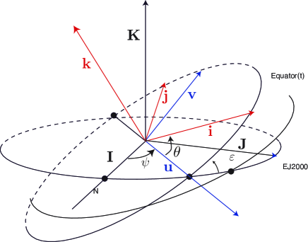
Figure 1:

Let us consider a planet ${\cal P}$ with momentum of inertia $A=B<C$ orbiting the Sun on a fixed ellipse (we will not consider here the planetary perturbations or the perturbations due to the satellite presence), and a satellite ${\cal S}$ of mass $m$ orbiting the planet. Let $({\bf i},{\bf j},{\bf k})$ be a basis linked to ${\cal P}$ with ${\bf k}$ associated to the axis of maximum inertia $C$. Let $({\bf I},{\bf J},{\bf K})$ be a fixed reference frame, with origine in the direction of ${\bf I}$, and ${\bf K}$ normal to the orbital plane of ${\cal P}$ (Fig.1). $a$ and $e$ are the semi-major axis and eccentricity of ${\cal S}$, $\Omega$ and $i$ the longitude of the axcending node of the satellite orbits over the orbital plane of the planet $({\bf I},{\bf J})$, while $v$ is the true longitude, and $\omega$ the argument of perihelion. If ${\bf r}$ is the radius vector from the planet’s to the satellite’s center of mass, with modulus $r$ and unitary vector ${\bf v}={\bf r}/r$, the torque exerteed by ${\cal S}$ on ${\cal P}$ is

$$\Gamma={{\displaystyle 3Gm}\over{\displaystyle r^{3}}}{\bf v}\wedge{\cal I}{\bf v}$$ (1)

where $G$ is the gravitational constant and ${\cal I}$ the matrix of inertia (${\cal I}={\rm diag}(A,A,C)$). Noting that ${\cal I}={\rm diag}(A,A,A)-{\rm diag}(0,0,C-A)$, (1) can also be expressed as (see Murray, 1983)

$$\Gamma=-{{\displaystyle 3Gm}\over{\displaystyle r^{3}}}(C-A){\bf k}\wedge({\bf v}{\bf v}^{\tau}){\bf k}$$ (2)

where ${\bf v}^{\tau}$ denotes the transposed of ${\bf v}$ (${\bf v}^{\tau}{\bf k}$ is thus the dot product of the two vectors ${\bf v}$ and ${\bf k}$). We will average $\Gamma$ over the fastest angle of this problem, that is over the mean anomaly $M$ of the satellite (the rotational angle $\theta$ is removed after the asumption $A=B$). As ${\bf k}$ does not depends on $M$, the only expression to average in (2) is $\gamma={{\bf v}{\bf v}^{\tau}}/{r^{3}}$. In the $({\bf I},{\bf J},{\bf K})$ frame, the coordinates of ${\bf v}$ are

$${\bf v}={\cal R}_{3}(\Omega){\cal R}_{1}(i)\left(\begin{matrix}{\cos(v+\omega)\cr\sin(v+\omega)\cr 0\cr\right)\end{equation}\end{matrix}with\begin{equation}\begin{matrix}{{\cal R}_{1}(\alpha)=\left(\cr\vskip 6.0pt plus 2.0pt minus 2.0pt\cr\end{matrix}}}$$ (10)