Single pulses from PSR B1641–45

Abstract

The integrated profile of PSR B1641$-$45 can be decomposed into four Gaussian components. The sum of these Gaussian components can be made to replicate the total intensity, linear and circular polarization of the integrated profile, and the discontinuity in the swing of the position angle. Surprisingly, the single pulses from PSR B1641$-$45 can also be decomposed into these same Gaussian components with only the amplitude of the components as a free parameter. The distributions of the fitted amplitudes are log-normal. Under the assumption that emission consists of 100% polarized orthogonal modes which are emitted simultaneously, I show that the polarization properties of the single pulses can also be replicated in a simple way. This lends support to models involving the superposition of orthogonal modes rather than disjoint emission of the modes.

1 Introduction

The integrated pulse profile from pulsars is one of the key characteristics of the emission process. Although single pulses vary widely both in intensity and shape, integrating a few thousand pulses produces a highly stable integrated profile. The integrated profile therefore yields clues as to the permanent structures associated with the pulsar magnetosphere. Kramer et al. (1994) showed that the integrated profile can be decomposed into a small number of Gaussian components. These components represent a 2-D Gaussian region of emission from a fixed height in the patchy pulsar beam [Lyne & Manchester 1988]. In single pulses, some fraction of the component is emitting when the beam sweeps the line of sight and therefore the single pulses tend to have narrower features (sub-pulses) than those of the integrated profile. The sub-pulse features may also rotate about the magnetic axis, producing the drifting sub-pulse phenomenology [Deshpande & Rankin 1999]. Integrated profiles show high levels of linear polarization and moderate circular polarization. Single pulses tend to be more highly polarized than the integrated profile. The smooth position angle swing in integrated profiles as a function of pulse longitude can occasionally be broken by 90° jumps which shows that the emission is present in two orthogonal modes of radiation. There has been considerable debate in the literature over whether these two orthogonal modes are emitted simultaneously or disjointly. Recently, McKinnon & Stinebring (1998) and Karastergiou et al. (2002) have shown that simultaneously occuring modes nicely explain many aspects of single pulse data.

PSR B1641$-$45 is one of the brightest pulsars in the sky at 1.4 GHz. It has a pulse period of 455 ms and its pulse profile consists of a single component preceeded by a low amplitude ‘precursor’. Previous observations of this pulsar at a frequency of 1.6 GHz by Manchester, Hamilton & McCulloch (1980) showed that it had moderate linear and circular polarization and that the leading ‘precursor’ had a high degree of linear polarization orthogonal to the polarization of the main pulse emission. Rankin (1990) and van Ommen et al. (1997) classify the pulsar as a core single even though it has a relatively shallow position angle swing across the pulse.

2 Observations and Data Reduction

As part of a project investigating single pulses from a large sample of pulsars, PSR B1641$-$45 was observed on 2000 March 16 and 17 using the 64-m Parkes radio telescope. The centre frequency, $\nu$, of the observations was 1413 MHz; at this frequency the system equivalent flux density is 26 Jy. The receiver consists of two orthogonal feeds sensitive to linear polarization. The signals are down-converted and amplified before being passed into the backend. The backend, CPSR, is an enhanced version of the Caltech Baseband Recorder (Jenet et al. 1997). It consists of an analogue dual-channel down-converter and digitizer which yields 2-bit quadrature samples at 20 MHz. The data stream is written to DLT for subsequent off-line processing allowing all 4 Stokes parameters to be computed. On the two occasions, 3102 and 3718 single pulses were recorded. Before each observation, a 90-s observation of a pulsed signal, directly injected into the receiver at a 45° angle to the feed, is made. This enables the gain of each channel and the phase difference between the channels as a function of frequency to be calibrated. Observations of the flux calibrator Hydra A were made which allows absolute fluxes to be obtained.

Figure 1: Integrated pulse profile at 1.4 GHz. Position angle is shown on top, and the total intensity (solid line), linear (dashed line) and circular (dash-dot line) polarizations are shown in the bottom panel. The location of time zero is arbitrary, but roughly aligns with the pulse peak.

Figure 2: The four Gaussians which make up the integrated profile of PSR B1641$-$45. The parameters are given in Table 1.

The data were processed off-line using a workstation cluster at the Swinburne Supercomputer Centre. Data reduction involves coherent de-dispersion (Hankins & Rickett 1975) and includes quantization error corrections as described by Jenet & Anderson (1998). The data are folded at the apparent topocentric period of the pulsar and the full Stokes profiles for each pulse are written to disk. Flux calibration and instrumental calibration are then carried out using information contained in the observation of the pulsed (calibration) signal. The data in each frequency channel is corrected for the rotation measure of the pulsar and all the frequency channels are then summed to produce the final profile. The final profiles consist of 1024 time-bins per pulse period for an effective time resolution of 0.44 ms.

3 Integrated Profile

Figure 3: The simulated profile of PSR B1641$-$45 constructed from the sum of the four Gaussians parameterised in Table 1.

The integrated profile of PSR B1641$-$45 is shown in Figure 1. The continuum flux density is 430 mJy and the peak of the profile has a flux density of 21 Jy. The pulsar shows a moderate amount of linear polarization ($\sim$20%) and a small amount of circular polarization ($\sim$6%), which is predominantly negative throughout. The position angle swings by about 50° throughout the main pulse. There is a ‘pedestal’ or ‘pre-cursor’ at the leading edge of the profile and the polarization of this feature is orthogonal to the rest of the pulse. The peak of the linear polarization occurs earlier than the peak in total intensity. These results are consistent with the observations of Manchester et al. (1980). There is scatter broadening of the pulse profile at this observing frequency although it is difficult to measure without knowing the underlying pulsar profile. As part of a separate study of this pulsar (Rickett et al. In preparation), we measured a pulse broadening time of 56 ms at an observing frequency of 660 MHz. This is an improvement over the only value currently in the literature, 40$\pm$10 ms at 750 MHz by Komesaroff et al. (1973). Extrapolating to $\nu$=1413 MHz by assuming that the broadening time scales as $\nu^{-4.4}$ yields a scattering time of $\sim$2.0 ms at the observing frequency used here. This time is small compared to the duration of the pulse, but likely manifests itself as the tail of the emission at times beyond 13 ms in Figure 1.

After accounting for the orthogonal mode jump, the rotating vector model (RVM) can be fitted to the position angle swing. As is commonly the case, the angles $\alpha$ (between the rotation and magnetic axes) and $\beta$ (the offset of the line of sight from the magnetic axis) are not well constrained, mostly because emission only occurs from a small fraction of pulse longitude. I adopt the parameters $\alpha=30\degr$, $\beta=8\degr$ with the magnetic pole crossing located at phase 0.931, just prior to the pulse peak. These parameters provide an adequate fit to the data, and their exact values are not crucial to the discussion below.

No	Amplitude	Location	Sigma	Linear	Circular
	(Jy)	(ms)	(ms)	fraction	fraction
1	0.43	–13.2	2.55	–0.6	0.0
2	3.49	–4.55	2.28	0.9	0.2
3	16.22	–1.36	2.41	0.15	–0.12
4	8.00	+2.73	3.96	0.13	–0.05

Table 1: Parameters of the components of PSR B1641$-$45 after Gaussian decomposition. The location of the peaks is relative to zero time as shown in Figure 1.

Kramer et al. (1994) demonstrated the method of decomposing the total intensity profiles of pulsars into Gaussian components and showed that typically fewer than five were necessary in the majority of cases. Applying this method to PSR B1641$-$45, I find that four Gaussian components provide the best fit to the data. The fit is excellent apart from the the trailing edge of the pulsar where scatter broadening of the profile is clearly seen. I define a Gaussian by

$$y=A\,\,\,e^{-\frac{1}{2}(\frac{x-\bar{x}}{\sigma})^{2}}$$ (1)

and list the parameters of the fitted Gaussians in Table 1. The fitted components are shown in Figure 2. The smallest amplitude component is necessary to fit the precursor. The location of the second Gaussian is close to the peak of the linear polarization. I therefore attempted to fit both the linear and the circular polarization by varying the fractional polarization in each of the four components. The results are listed in Table 1. Note that the linear polarization of the precursor is negative which implies that it is orthogonally polarized to the rest of the emission. The position angle at a given longitude is computed from the parameters of the RVM fit given above. The appropriate values of Stokes $Q$ and $U$ are then computed from the position angle for each Gaussian. These are then summed to produce the integrated Stokes $Q$ and $U$ which are then re-converted back to position angle. The profile of the ‘simulated’ pulsar is shown in Fig. 3. The simulated profile can be compared directly with Fig. 1; in particular the simulated profile nicely reproduces most of the main features of the real profile, including the location of the orthogonal mode jump which occurs when the amplitude of Gaussian 1 drops below that of Gaussian 2. Also, both the linear and circular polarizations match well with the true values.

4 Single Pulses

4.1 Total Intensity

Figure 4: Examples of single pulse fitting. Both panels show the observed data with a dashed line. The three fitted Gaussians are shown with a solid line as is the sum of these Gaussians. Top panel shows a strong pulse whose components have amplitudes 6.2, 24.7 and 12.6 Jy. Lower panel shows a weak pulse with component amplitudes 3.6, 9.6 and 7.5 Jy.

Figure 5: Flux distribution of Gaussian 4 fitted to the single pulse data. Best fit is shown as a solid line.

The single pulses from this pulsar are rather featureless. They generally show a similar morphology to that of the integrated profile and there is no evidence for microstructure or drifting sub-pulses as is the case for many other pulsars. The precursor component seen in the integrated profile is rarely seen in the single pulses as the noise dominates its emission.

Given the similarity between the single pulses and the integrated profile, I attempted to perform Gaussian decomposition on the single pulses. Most recently, Gupta & Gangadhara (2003) have applied a ‘window-thresholding’ technique to single pulse data. This allowed them to detect extra components in the pulse profile which they then Gaussian fitted to obtain their parameters. Here, I adopt a slightly different technique. The width and centroid of the gaussians are fixed to the values obtained from the fit to the integrated profile as it seemed apparent from visual inspection that the single pulses had the same pulse width as the integrated profile. However, the low amplitude Gaussian necessary to fit the precursor region of the integrated profile was not included as it is too weak to be seen in single pulses and thus could not be constrained in the fitting process. I therefore performed fitting to the single pulses with three free parameters (the amplitude of the three Gaussians listed as 2-4 in Table 1). This provided good fits (as judged by the $\chi^{2}$ statistic) to the single pulse data in more than 95% of the cases. The majority of the failures came when the flux density of the pulsar was low. Often, the amplitude of Gaussian 2 was very low and the single pulses were just as adequately fit with two Gaussians. However, some pulses required a high amplitude for Gaussian 2.

The scatter broadening of the pulse is not taken into account in the fitting procedure in that symmetrical Gaussians rather than scatter broadened Gaussians are used. The scattering only affects the tail of the profile, where the signal to noise ratio is low. However, the goodness of fit is weighted towards the high signal to noise points (i.e. the pulse peak). The fitting procedure is therefore largely unaffected by the scattering. I return to the effects of scattering on the implications of the results in a later section. Figure 4 shows two examples of single pulses and the fitted Gaussians. The fits are excellent and show that the scatter broadening is not playing a significant role in determining the fitted parameters.

The question then arises as to the distribution of the amplitudes of the Gaussians. Figure 5 shows the distribution for Gaussian 4. The distribution is clearly log-normal with a mean amplitude of 16.7 Jy and a $\sigma$ of 0.27 (in the log). Similarly, Gaussian 3 is log-normally distributed with a mean of 38.7 Jy and a $\sigma$ of 0.13 (in the log). The statistics of Gaussian 2 are more problematical to determine as often this component is weak and hence dominated by noise. A reasonable fit is obtained with a log-normal distribution with a mean of 7.45 Jy and a $\sigma$ of 0.3 in the log. Note that the means obtained in the fitting process correspond nicely to the peak amplitudes obtained during the Gaussian decomposition process on the integrated profile. This gives confidence that the fitting procedure is working correctly. Remarkably, therefore, the single pulses from this pulsar can be reproduced by drawing three random numbers from the above distributions and summing the resultant Gaussians together.

No	log(Amp 1)	log(Amp 2)	Sigma	Corr Coeff	Circular fraction	Circular spread
1	–0.189	0.421	0.00	0.7	0.0	0.15
2	0.451	–0.829	0.27	0.7	0.2	0.15
3	0.941	0.811	0.13	0.7	–0.12	0.15
4	0.571	0.461	0.27	0.7	–0.05	0.15

Table 2: Parameters used in the simulation of single pulses from PSR B1641$-$45

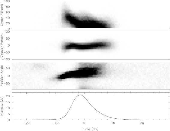
Figure 6: Grey-scale representation of the polarization properties of the single pulses from PSR B1641$-$45. Black denotes regions of high counts.

4.2 Polarization

In order to examine the polarization of the single pulses, an analysis similar to that of Stinebring et al. (1984a,b) was performed. For the linear polarization, for example, a two dimensional grid is constructed with the pulse phase along the x-axis and 20 bins along the y-axis from 0 to 100%. For each pulse the appropriate cell is then updated by one depending on its linear polarization. The same procedure is carried out for the circular polarization and the position angle. The values in the cells are then converted to a linear grey-scale between white and black depending on the counts in that cell. Figure 6 shows the grey-scale representation of the data. The figure shows that although there is a large spread in the linear and circular polarization, rather few pulses have a net polarization greater than 50% apart from the leading edge of the profile. There is also little evidence of orthogonally polarised modes in the position angle distribution.

Figure 7 shows the polarization properties of the phase bin where the linear polarization is maximum. In this bin, one mode dominates virtually all the time, the position angle distribution is narrow around its mean value. The fractional linear polarization is high and the circular polarization shows large flux densities of either sign although there is a slight preference for negative values. This contributes to give a low net circular polarization.

Figure 8 shows the same information for a phase bin on the trailing edge of the profile. Both the total intensity and linearly polarized intensity are lower as is the fractional linear polarization. The PA distribution is much broader than seen in Fig. 7. This is partly due to increased uncertainity in the measurement of the PA (as the linear polarization is lower) and partly due to the presence of the orthogonal mode appearing near PA $-80\degr$. The circular polarization is more evenly distributed around zero.

5 Simulating Single Pulses

I have already demonstrated that replicating the single pulses in total intensity is a relatively simple task for this pulsar. It involves drawing three random numbers from a log-normal distribution. What further parameters need to be added in order to replicate the polarization of the single pulses?

As a starting point I use the model proposed by McKinnon & Stinebring (1998). In their model both polarization modes are emitted simultaneously and are 100% polarized. Then, the total power is the sum of the intensities of the two modes and the linear polarization is their difference. The amplitudes of the modes are highly correlated. They found that, under these assumptions, the single pulse data of Stinebring et al. (1994) could be replicated. McKinnon & Stinebring (1998) treated each phase bin in an independent fashion. In a further paper, they also showed that the integrated profile could be ‘split’ into the two orthogonal modes [McKinnon & Stinebring 2000]. This involved a simple mathematical manipulation based on the fractional linear polarization in each bin (see also Karastergiou et al. 2003).

In this instance, I assume that the Gaussians described in Section 3 are a coherent emitting unit, or patch, and that they emit radiation simultaneously in two, 100% polarized orthogonal modes. Ignoring for now the circular polarization, one can apply the technique of McKinnon & Stinebring (2000) to compute the mean amplitude of each of the modes for each of the Gaussians under these assumptions using the data from Table 1 and knowing the integrated fractional polarization. Furthermore, the distribution of the amplitudes of these Gaussians are also known from the fitting described above; they are all log-normal.

Figure 7: Polarization properties of bin at time –3.4 ms. Flux density in Jy, position angle in degrees. The 1-$\sigma$ noise is level is 0.6 Jy.

Figure 8: Polarization properties of bin at time 3.64 ms. Flux density in Jy, position angle in degrees. The 1-$\sigma$ noise is level is 0.6 Jy.

In order to simulate the polarization of the single pulses from PSR B1641$-$45, therefore, we now need to draw 8 random numbers (one pair for each of the Gaussians in the table) from a log-normal distribution with the mean and sigma as given in Table 2. Note that the random values for each mode are correlated according to the correlation coefficient given in the table [McKinnon & Stinebring 1998]. Also, the parameters for Gaussian 1 are not well constrained, but do not play a major role in the single pulse data as the flux density is low. The total intensity of each Gaussian is then the sum of the amplitudes of the two orthogonal modes and the linear polarization is the difference of their amplitudes. This accounts for the linear polarization but does not include any circularly polarized component. The mean circular polarization of each individual Gaussian is already known from the fits to the integrated profile. It is tempting to associate a handedness of circular polarization with a given orthogonal mode as has been proposed by e.g. Cordes, Rankin & Backer (1978). However, this seems be to true only at observing frequencies lower than $\sim$600 MHz. Recent observations of the Vela pulsar [Kramer, Johnston & van Straten 2002] and PSR B1133+16 [Karastergiou, Johnston & Kramer 2003] show that the situation is much more complex at frequencies above about 1 GHz. There is a lack of correlation between the handedness of circular polarization and the dominant orthogonal mode, but a rather large spread in the values of both hands of circular polarization. For each component (not each orthogonal mode), I therefore draw the circular polarization from a Gaussian distribution with a mean and standard deviation as listed in Table 2.

Figure 9: Simulated data from the same time bin as in Fig 7.

Figure 10: Simulated data from the same time bin as in Fig 8.

Single pulses simulated in such a way bear a strong resemblance to the true single pulse data. Figs 9 and 10 show the simulated data for the same phase bins as Figs 7 and 8. Comparison between the total intensity distributions show that the low flux density pulses are under-represented, however the high intensity data are well matched. The linear and circular polarizations are well replicated. The biggest discrepancy lies in the spread of the position angle distributions. In the simulated data, the spread is relatively narrow and the orthogonal modes are well separated. The spread in values is almost entirely due to receiver noise as I have assumed that the position angle is fixed for a given bin. In the real data the spread is much larger than a delta function convolved with the noise. This is similar to the results found by McKinnon & Stinebring (1998) and Karastergiou et al. (2002).

6 Discussion

I have shown that Gaussian decomposition of the integrated profile not only provides a good fit to the total intensity but can also fit the polarization profile, including the location of the orthogonal jump. In this pulsar, at least, these same Gaussians can be made to fit the single pulse data with only their amplitudes as a free parameter. Interestingly the distribution of these amplitudes is log-normal. Log-normal distributions are seen both in the time-averaged flux density of pulsars and in phase resolved statistics [Cairns, Johnston & Das 2001, Cairns, Johnston & Das 2003]. The implications are then that pulsar emission may be interpreted in terms of stochastic growth theory and that the emission mechanism is linear, involving either a direct linear instability or linear mode conversion of non-escaping waves driven by a linear instability as discussed in detail in Cairns et al. (2003).

Under the assumptions of 100% polarized orthogonal modes, the polarization distributions of the single pulse data can also be reproduced from a relatively small number of random variables. This extends the work of McKinnon & Stinebring (2000) by implying that the sub-pulses can be characterised in such a way (not just a particular phase bin) and that log-normal statistics are clearly the dominant statistic for the observed flux density distributions. Any physical model must therefore have as its basis an emission beam which is 100% polarized and which is subsequently split through e.g. bi-refringence into two orthogonally polarized modes. However, it is clear that propagation effects, not taken into account in the simulation process, strongly affect the position angle and the degree of circular polarization seen in single pulses. This situation has also been seen previously by a number of observers and discussed in the context of theoretical models by Petrova (2001). In her model, the polarization modes recombine in the ‘polarization limiting region’. This mode coupling then allows for significant deviations in the position angle and in the circular polarization, with greater position angle deviations leading to increased circular polarization. The data here do not entirely support this picture. Comparison between Figs 7 and 8 show that the former has a much narrower spread of position angles than the latter but that the percentage V distributions look very similar. The effects of refraction in the magnetosphere are also likely to be important as the two modes are affected differently. This is likely to result in a mode mixture at a given observer’s longitude and such an effect would also serve to broaden the position angle distribution.

The applicability of this method to other pulsars is not clear. For example, in the Vela pulsar, Krishnamohan & Downs (1983) showed that four Gaussian components fitted the total intensity data and could account for some of the single pulse data. More recent observations with much higher time resolution [Kramer, Johnston & van Straten 2002] showed that microstructure was prevalent in the single pulse data. Clearly, no amount of Gaussian fitting will reproduce microstructure. Other pulsars, such as PSR B0950+08 show a bewildering variation in the amplitude and location of single pulse components, and there is almost no resemblance between the single pulses and the integrated profile. Many pulsars, such as PSR B1133+16, show orthogonal mode jumps near the peak of a pulse component and again such a feature is hard to reproduce using simple Gaussian decomposition.

However, it may be that there is a class of pulsars similar to PSR B1641$-$45 for which this method will work very well. One possibility is that the scatter broadening in this pulsar blurs the features with time-scales less than the sub-pulse time. The same was also true of the low resolution observations of the Vela pulsar where the dispersion measure smearing also blurred out the microstructure. Processing techniques which involve smoothing over the microstructure are also possible. For example, van Leeuwen et al. (2002) fitted Gaussian components to PSR B0809+74 in order to study the drift bands and noted how similar the Gaussians were in amplitude and width.

It therefore appears to be possible to get a handle on processes on the scale of tens of milliseconds (the subpulses) without delving into the complexities which occur on timescales significantly shorter. The data seem to favour the idea of simultaneously occuring modes of emission, with propagation through the magnetosphere influencing the degree of circular polarization and the position angle variations.

References

- [Cairns, Johnston & Das 2001] Cairns I. H., Johnston S., Das P., 2001, ApJ, 563, L65
- [Cairns, Johnston & Das 2003] Cairns I. H., Johnston S., Das P., 2003, MNRAS, Submitted
- [Cordes, Rankin & Backer 1978] Cordes J. M., Rankin J. M., Backer D. C., 1978, ApJ, 223, 961
- [Deshpande & Rankin 1999] Deshpande A. A., Rankin J. M., 1999, ApJ, 524, 1008
- [Gupta & Gangadhara 2003] Gupta Y., Gangadhara R. T., 2003, ApJ, 584, 418
- [Karastergiou, Johnston & Kramer 2003] Karastergiou A., Johnston S., Kramer M., 2003, AA, 404, 325
- [Karastergiou et al. 2002] Karastergiou A., Kramer M., Johnston S., Lyne A., Bhat R., Gupta Y., 2002, AA, 391, 247
- [Komesaroff et al. 1973] Komesaroff M. M., Ables J. G., Cooke D. J., Hamilton P. A., McCulloch P. M., 1973, Astrophys. Lett., 15, 169
- [Kramer, Johnston & van Straten 2002] Kramer M., Johnston S., van Straten W., 2002, MNRAS, 334, 523
- [Kramer et al. 1994] Kramer M., Wielebinski R., Jessner A., Gil J. A., Seiradakis J. H., 1994, A&AS, 107, 515
- [Krishnamohan & Downs 1983] Krishnamohan S., Downs G. S., 1983, ApJ, 265, 372
- [Lyne & Manchester 1988] Lyne A. G., Manchester R. N., 1988, MNRAS, 234, 477
- [Manchester, Hamilton & McCulloch 1980] Manchester R. N., Hamilton P. A., McCulloch P. M., 1980, MNRAS, 192, 153
- [McKinnon & Stinebring 1998] McKinnon M., Stinebring D., 1998, ApJ, 502, 883
- [McKinnon & Stinebring 2000] McKinnon M. M., Stinebring D. R., 2000, ApJ, 529, 435
- [Petrova 2001] Petrova S. A., 2001, AA, 378, 883
- [Rankin 1990] Rankin J. M., 1990, ApJ, 352, 247
- [Stinebring et al. 1984a] Stinebring D. R., Cordes J. M., Rankin J. M., Weisberg J. M., Boriakoff V., 1984a, ApJS, 55, 247
- [Stinebring et al. 1984b] Stinebring D. R., Cordes J. M., Weisberg J. M., Rankin J. M., Boriakoff V., 1984b, ApJS, 55, 279
- [van Leeuwen et al. 2003] van Leeuwen A. G. J., Kouwenhoven M. L. A., Ramachandran R., Rankin J. M., Stappers B. W., 2003, AA, 387, 169
- [van Ommen et al. 1997] van Ommen T. D., D’Alesssandro F. D., Hamilton P. A., McCulloch P. M., 1997, MNRAS, 287, 307