Quasar Atmospheres: Toward a ‘Low’ Theory for Quasars

Abstract

After 40 years we have no ‘low’ theory of quasars to predict the atomic absorption and emission features so abundant in quasar spectra. Here I take the first step, using results selected for their diagnostic power to build an ‘observational paradigm’ unifying all the atomic features in quasars. This paradigm bears a remarkable resemblance to the one I proposed in Elvis (2000)! Yet all the results used here were not used in that earlier study, with one exception. The Elvis (2000) model has been tested by the new data and has survived, and so has been strengthened. The structure is readily tested, is physically suggestive, and opens up many areas for detailed modelling. From this I believe a truly predictive ‘low’ theory of quasars will emerge.

Harvard-Smithsonian Center for Astrophysics, 60 Garden St., Cambridge MA 02138 USA

1. INTRODUCTION: HIGH THEORY AND LOW

Enlightenment does not scale with published mass. The quasar/AGN literature has over 12,000 refereed published papers, and papers now appear at a rate of about 2/day. Yet few would contend that we have a much deeper understanding of quasars today than we did 30 years ago. By 1974, just over 10 years after the discovery of quasars, all of the current model for a quasar were in place: a central massive black hole, an accretion disk and a relativistic jet. We have made great observational progress mapping out quasar properties at all wavelengths, and in the Unified Scheme (Padovani & Urry 1999) have resolved much of the confusing properties of quasars to be due to the effects of obscuration. But most quasar observations are of atomic features. The black hole/disk/jet theory is a ‘high’ theory, dealing only with overall energetics, and describes a naked quasar, devoid of any of the veiling gas that creates these atomic features. We need a ‘low’ theory with sufficient detail to predict the emission and absorption phenomenology of quasars. But to get to such a theory in one step from 10⁴ papers is not realistic. First we need to build an ‘observational paradigm’ to unify the phenomenology into a coherent, over-constrained, and so robust, structure of what can accurately be called the quasar atmosphere.

2. THE BLIND MEN AND THE ELEPHANT: GETTING THE QUASAR BIG PICTURE

In the old Indian tale six blind men approach an elephant to understand what it might be. The first happened on the elephant’s flank and declared that an elephant is a wall; the second found the tusk and pronounced an elephant to be a spear; the third grasped the trunk, and decided an elephant was a snake; the fourth felt a leg, and called an elephant a tree; the fifth touched an ear and decided that an elephant is a fan; and the sixth seized the tail and so said an elephant is a rope. Each was confident in his diagnosis, “Though each was partly in the right, And all were in the wrong!”. Moral: Not using all the available information can be quite misleading. So when we study quasar atmospheres we must not look at just one wavelength or feature, but must consider all the features together (table 1).

Table 1.: Quasar Atmosphere Features

Broad Emission Lines	BELs
which we can divide into:
High Ionization Broad Emission Lines	HIBELs
Low Ionization Broad Emission Lines	LOBELs
Broad Absorption Lines	BALs
Narrow Absorption Lines	NALs
X-ray Warm Absorbers	WAs
Scattering phenomena (BAL troughs, VBELR, Compton Humps, Fe-K)

3. A PARADIGM FOR QUASAR ATMOSPHERES

In Elvis (2000) I proposed a simple paradigm for quasar atmospheres. To the high theory combination of black hole/disk/jet, I added a wind arising from the accretion disk (figure 1). The wind has specific properties: coming from a restricted range of radii, initially making a large angle to the disk plane (and so being roughly cylindrical), and becoming radial well above the disk, making a $\sim$60^∘ angle to the disk axis to form a hollow bi-cone.

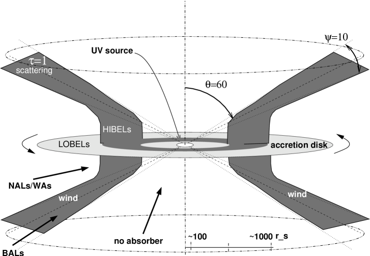
Figure 1.: A Paradigm for Quasar Atmospheres (Adapted from Elvis 2000)

Looking through the quasi-cylindrical part of the wind we see NALs and WAs (Table 1). Because we are looking through a flattened structure, scattering off the wind produces polarization. When we look near to the rotation axis our line of sight misses the wind altogether and we see no absorption features. We are also looking down on a highly symmetric structure, so polarization is weak. A cool phase of this wind emits the HIBELs. The LOBELs come from the outer disk. As the wind becomes radial it is accelerated; looking down the radial through this accelerating gas we see the BALs. The BAL wind is marginally Thompson thick, producing the observed electron scattering signatures.

This model is purely geometric and kinematic. At first this appeared to be a weakness. We all want to go directly to the physics of this wind. But let’s recall that the Rees model for relativistic jets was also just a geometric and kinematic model. To this day we do not have an accepted theory of quasar jet acceleration, yet the simple model allows us to understand quite a bit. Intermediate models or paradigms such as these are valuable. Note also that this model is independent of the type 1/type 2 Unified Scheme. An obscuring torus at large radii would simply shrink the opening angle derived for the bi-cone.

Several features of quasar atmospheres fall out as a natural consequence of the structure proposed in Elvis (2000) [e.g. the BAL covering factor; BAL ‘detachment velocities’; HIBEL blue-shifts.] This is encouraging. In the following I reconstruct the same paradigm using only studies not used in Elvis (2000), except one. The fact that the structure can be re-built with almost none of the original starting blocks is itself a strong test of the model and suggests that there is something to it.

4. FILTERS: Finding Observations with Leverage

Since there are so many papers on quasars we need a means to filter out the many which do not point us toward a paradigm . I use three filters to accept papers: (1) Physical measurements. e.g. Mass, length, density, (but not ratios, column densities). (2) Absorption lines. Since absorption only involves an integration of the gas distribution over one spatial dimension, not three, and because the sign of one of the three velocity dimensions is also determined (i.e. blue-shift = outflow), which is not true for emission lines. (3) Polarization. Since any polarization implies a non-spherical geometry and quasars, unlike stars, are not spherical even to first order. (As we know from their jets.)

5. PHYSICAL MEASUREMENTS

5.1. A Rotating, Large Scale-Height BEL Region

Reverberation mapping of the BELs has been the most valuable technique in quasar/AGN work. As a means of understanding quasar atmospheres the most important result is the radius-line width relation for BELs (Peterson & Wandel 2000). This correlation follows a Keplerian $v^{2}r=constant$ relation, which tells us that the BEL gas is close to bound and close to following simple orbits. Peterson (2003, these proceedings) demonstrates that there are still factors of 2-3 uncertainty in the normalization of $v^{2}r$ to black hole mass, so that pure Keplerian motion is not required. However, the lack of red-blue asymmetry in the reverberation response in NGC 5548 (Wanders et al. 1995) already requires a large orbital component, as does the polarization of H$\alpha$ (Robinson et al. 2002).

Variability of another kind - VLBI expansion - lets us derive another physical measurement, the angle of the jet axis to our line of sight, $\theta$, (figure 1, assuming we know $H_{0}$). Rokaki et al. (2003) use this approach to derive jet angles for a sample of radio-loud quasars for which they also measure H$\alpha$ FWHM and equivalent widths (EW). Strikingly they find angles up to 40^∘, well away from the region ($\theta<10\hbox{${}^{\circ}$}$) where a beamed continuum dominates the quasar spectrum. Rokaki et al. find that more edge-on objects have on average broader FWHM(H$\alpha$), implying ordered rotation around the jet axis. Similar correlations with radio core-to-lobe ratio, which is a proxy for $\theta$, find the same result, but proxy measurements cannot compare model predictions. Having $\theta$, Rokaki et al. can do so, and they find that pure rotation is not a good fit, and that another component of amplitude $\sim$2000 km s^-1 is needed. We return to this later (§6.3).

The EW(H$\alpha$) vs $\theta$ plot also shows a correlation. If H$\alpha$ were from a flattened disk, as we expect the continuum to be, then as we view the disk at larger and larger angles both would suffer the same geometric and limb darkening, and so no change in EW. Instead larger $\theta$ objects have larger EW(H$\alpha$). Rokaki et al. find that the EW vs. $\theta$ relation is just as expected if the continuum comes from a disk and suffers cos $\theta$ and limb darkening, but the H$\alpha$ is isotropic. So the BEL is not only rotating, it also has a large scale height, rising well above the continuum producing disk. I.e. a rotating cylinder.

A rotating cylinder is not an equilibrium configuration. A Keplerian velocity on the disk becomes super-Keplerian above the disk, so gas there will feel a radial centrifugal acceleration. A natural way of producing this configuration is for BEL gas to be a wind rising off the disk at a large angle to the disk.

5.2. A Limited Range of BEL Wind Radii

The reverberation mapping FWHM vs lag time correlation shows that the BEL region is stratified, with HIBELs (Table 1), which have FWHM$\leq$10,000 km s^-1, lying in the inner region at $\sim$1000 $r_{s}$ ($r_{s}$=Schwartzchild radii). For NGC 5548 (Korista et al. 1995) the ratio of the HeII to CIV lag times is roughly 3, so the HIBEL region has an approximate thickness $\Delta r/r\sim$3, although at this level it is not obvious how to define the correct lags (Peterson 2003, these proceedings).

Collin-Souffrin et al. (1988) proposed that the LOBELs (Table 1) come from a disk, while the HIBELs come from a large scale height flow. Since the LOBELs are narrower and have longer reverberation times, they lie outside the HIBEL region. Once we think of the HIBELs as coming from a wind, the Collin-Souffrin et al. picture requires that the HIBEL wind arises only from a restricted range of radii. This idea is strongly supported by observations of two Narrow Line Seyfert 1s (NLSy1s) by Leighly & Moore (2003). They find that the LOBEL MgII is narrow and symmetric, as implied by the NLSy1 label, but that the HIBEL CIV is broad and asymmetric to the blue. This is readily explained if the CIV velocity comes from a wind, with the far (red-shifted) side of the wind obscured by the disk. Similar blueshifts of HIBELs relative to LOBELs have been known for a long time in ordinary quasars (Gaskell 1982) but have remained puzzling. These can now be understood as less extreme examples of the effect found by Leighly & Moore. In normal quasars the HIBELs are dominated by disk rotation, but include blue-shifts of $\sim$1000-3000 km s^-1 due to a wind component. The lack of HIBEL redshifts seems to put the wind at accretion disk dimensions, not on a torus scale.

6. ABSORPTION

6.1. The NAL/WA gas: a 2-phase medium in Pressure Balance

The idea that the NALs and WAs came from the same medium was contentious only recently (Crenshaw 1997). Now that we have high resolution (R$>$400) X-ray spectra of quasars from Chandra and XMM-Newton, this concern has been laid to rest. The NALs and WAs both have (1) narrow line widths, (2) similar outflow velocities of $\sim$1000 km s^-1 (Collinge et al. 2000), (3) closely related ionization states (Krongold et al. 2003), and (4) occur in the same objects so reliably that one can predict the other (Mathur et al. 1998). So now we can use this equivalence to learn more about the UV/X-ray revealed winds from quasars.

Krongold et al. (2003) find 2 ionization states in the X-ray absorption spectrum of NGC 3783, and can exclude an intermediate third state. This points away from a many-phase medium (Krolik & Kriss 2001). The Krongold et al. model requires only 6 free parameters to fit over 100 X-ray absorption features (75% of which are blends). Occam’s razor says there is something to their model. They find that the pressure in the two gases is equal, assuming only that they lie at the same distance from the central continuum, as is suggested by their shared kinematics. When the two phases are plotted in temperature, T vs $\Xi$ (the ratio of radiation pressure to gas pressure) space they lie on the equilibrium curve for a gas illuminated by a continuum similar to that of NGC 3783. Netzer et al. (2003) find a 3rd, higher ionization, absorber and this may lie on the upper branch of the equilibrium curve. Krongold et al. (2004) have now found a similar solution for another object, NGC 985, so the result may be general. The cool phase has T$\sim$10⁴K, comparable to the BEL gas, and also has a similar ionization parameter, $log~{}U\sim$ -0.8. Hence a simple 2-phase medium in pressure balance is strongly indicated. Only an extraordinary coincidence could be invoked to explain the equal pressures if separate media are involved. The geometrical relation of the 2 phases is unknown: e.g. is it layered or foam-like.

6.2. The NAL/WA gas: a Transverse Wind, Close to the Continuum

How is the NAL/WA wind flowing? There is strong evidence that the primary motion is transverse to our line of sight; so the true speed of the wind is larger than the observed values. Arav et al. (2002) note that the CIV doublet ratio in NGC 5548 is not 2:1 as required by atomic physics. The only way out is to have extra continuum fill in the base of the absorption lines. But Arav et al. also find that the CIV doublet ratio varies systematically with velocity across the lines, so scattering into the line of sight is untenable. The only remaining possibility is that the absorbing gas covers different fractions of the continuum source at different velocities. A radial wind cannot do that unless our line of sight is very special. A transverse wind can naturally incorporate velocity-dependent covering factors if the wind accelerates across the diameter of the source. This requires the wind to be quite close to the continuum source, say within $\sim$10 continuum diameters (so that the continuum source subtends $>$10^∘) since at larger distances: (1) partial covering is improbable, (2) significant acceleration in a random small section of the wind is unlikely. A systematic change in covering factor with velocity also points to sheets rather than to a mist of clouds.

So the NAL/WA gas must lie in a transverse wind, close to the continuum, at $\leq$1000$r_{s}$ if the UV continuum comes from $\sim$100$r_{s}$. [$T=3\times 10^{4}$K for $L=0.05~{}L_{Edd},M_{\bullet}=10^{8}~{}M_{\odot}$ (Frank, King & Raine 1992, Eq.7.18) for NGC 5548 parameters (Peterson & Wandel 2000).] Limited WA variability monitoring gives similar sizes from recombination times (Nicastro et al. 1999). A transverse flow also implies a plane of origin and a conical or cylindrical structure.

6.3. One Wind: Combining HIBELs and NALs/WAs

In the above sections we have seen that the BEL is a wind, as is the NAL/WA. We also saw that the BEL and the NAL/WA winds both: (1) rise from a disk at a large angle; (2) lie roughly at $r\sim 1000~{}r_{s}$; (3) have the same pressure; (4) have complementary ionization parameters; (5) have non-orbital velocities of $\sim$1000-3000 km s^-1. In addition the BEL wind is rotating, something we do not know for the NAL/WA wind. The obvious simplest explanation is that the BEL is just the cool phase of the NAL/WA gas. There is only one disk wind from quasars, and it accounts for all the atomic features discussed so far.

7. POLARIZATION: A THOMPSON THICK SCATTERER

7.1. The NAL/WA Wind is Flattened and Universal

The optical polarization of AGN with NALs is higher than that of non-NAL AGN (Leighly et al. 1997). In a plot of % polarization vs. $log~{}N_{H}$ (from ASCA X-ray spectra) Leighly et al. find a clear separation between low $N_{H}$ non-NAL objects (with low polarization, $<$1%), and high $N_{H}$ NAL objects (with high polarization, $\sim$1-5%). The scatterer in the NAL objects must be highly flattened and seen close to edge-on. If follows that there must be objects from the same population seen pole-on, but these objects cannot be obscured by a large $N_{H}$ as there are no high $N_{H}$/low polarization objects. So the scatterer and the obscurer share a flattened co-axial geometry. The simplest explanation is that the scattering structure is a part of the NAL/WA (and by implication HIBEL) wind, and all AGN have NAL/WA winds. Yet the NAL/WA wind $N_{H}$ is only $\sim$10²²cm^-2, $\sim$1% of ${\large\tau}_{T}$, insufficient to produce strong polarization.

7.2. All Quasars have Flattened BAL Winds

BALs have widths $\sim$3-10%$c$, some 10 times those of NALs. BALs are only seen in $\sim$15% of quasars (Tolea, Krolik & Tsvetanov 2002). However BALs are of much wider importance in quasars because the strong polarization of the BAL troughs (Ogle et al. 1998) implies that BAL winds are highly flattened (Ogle 1998) and so must be present in all, or most, quasars. (This is the argument also used in Elvis 2000.)

If BAL winds are present in all quasars, but in most cases do not enter our line of sight, then non-BAL quasars should also show evidence of scattering off high velocity material. Ogle (1999, PhD thesis and unpublished preprint) uses a formalism for polarization from scattering off axisymmetric structures, first developed for Be stars, to show that a wide angle bi-cone (half opening angle $\sim 60$^∘), viewed from a random set of directions, can reproduce the distribution of optical polarization seen in non-BAL quasar samples. The implied universality of BALs in quasars and their 15% occurrence rate require the BAL bi-cone divergence, $\psi$, angle to be small.

BAL winds are then an integral part of quasar structure, and any model of quasar structure must include them. But we just showed that NAL/WA winds are universal in AGN. Is there a connection?

8. A BEND IN THE WIND: WA/NAL/HIBEL and BAL Unity

If the NAL/WA/HIBEL wind is transverse and forms a bi-conical structure (see §§6.2, 7.1), then there must be some cases where we look through the wind right down the flow direction. How many cases there are will depend on the wind divergence angle, $\psi$. $\psi$=10^∘(for $\theta$=60^∘, figure 1) gives a 15% covering factor for the central continuum source, so if this is the correct divergence angle then BALs could be simply the WA/NAL/BEL wind seen end on. The acceleration of the wind would show up in the broad profiles of the BELs. There is a problem with this picture. In a simple bi-cone with a 60^∘opening angle the typical NAL velocities will be $\sim$ 90% of the BAL velocity, instead of the 10% observed.

Why should BALs not simply be the high terminal velocity/high luminosity tail of the NAL population? After all, BALs are typically found in luminous quasars (at z$>$2 in order to see CIV BALs in ground-based optical spectra), while no low luminosity (low z) objects have NALs with widths $>$4000 km s^-1 (Kriss 2001). This is not a conclusive argument, as low luminosity sample sizes are typically only of order 20, so that only $\sim$3 BALs are expected. The larger samples of FUSE AGN, and Sloan Digital Sky Survey (SDSS) faint quasars at z$>$2 will test this idea more strongly. Meanwhile it is useful to consider alternatives.

A curious feature of BALs is their ‘detachment velocity’. The onset of a BAL is usually sharp, but does not occur at the center of the corresponding BEL, but offset to the blue by 0-4000 km s^-1. There are three potential explanations: (1) the BAL wind accelerates impulsively leaving negligible $N_{H}$ from 0-4000 km s^-1; (2) the BAL flow is initially over-ionized as it begins to accelerate, so line driving is weak (see §5.2) and the wind must be hydromagnetic. (3) The BAL flow bends into our line of sight only when it has already accelerated to some significant fraction of the BEL FWHM velocity.

The latter, geometrical, explanation is simple, and implies that low velocity NALs must be observed, since a bend in the wind allows many viewing directions to cut through a point in the wind at a large angle to the wind flow direction (figure 1), picking out a single velocity. If we accept a bend in the wind then we combine the NAL/WA/HIBEL wind with the BAL wind by a simple geometry.

If this unification is real we would expect evidence for high ${\large\tau}_{T}$ and BAL velocity material in low luminosity quasars (=AGN). The non-variable ‘narrow’ Fe-K X-ray emission lines, and their corresponding Compton humps, show that ${\large\tau}_{T}\sim$1 material is present in AGN far from the X-ray source (e.g. Chiang et al. 2000). Polarization and variability studies of BELs reveal a “Very Broad Emission Line Region” or VBELR. These broad faint wings are mainly seen in H$\alpha$ and are polarized (Young et al. 1999). This indicates that they are scattered radiation off electrons moving at about twice the FWHM(H$\alpha$). BALs typically have twice the BEL FWHM (Lee & Turnshek 1995), suggesting that the scattering material could well be the BAL gas. Since the VBELs do not vary, a scatterer larger than the HIBEL region, consistent with the conical BAL part of the wind, is a simple explanation. SDSS spectra (Hall et al. 2002) show that the occasional detachment velocities that lie redward of the peak of the emission lines can be explained by a rotating BAL wind close to an extended continuum source. Why the wind bends outward will be discussed in §9.2.

8.1. Return to a Paradigm for Quasar Atmospheres

With the above arguments we have constructed the same basic picture of quasar atmospheres proposed by Elvis (2000, see §3), out of almost entirely new results. All the components of quasar atmospheres listed in table 1 are included. The model explains several features not built in, which were previously just puzzling observed facts. The Elvis (2000) model has survived numerous tests: any of the data used above could have been inconsistent with the model, but did not turn out to be. This paradigm makes predictions, allowing stronger tests.

9. THE BEGINNINGS OF A LOW THEORY OF QUASARS

Given the growing solidity of the Elvis (2000) observational paradigm, we can begin to explore the physical implications. The realization that quasar atmospheres are not static but are winds, marks a big change in viewpoint. Winds not only point to specific physics for quasar atmospheres, they also allow us to think about the constraints they put on the base of the wind, i.e. the accretion disk. Winds also force us to ask what happens to the wind material as it leaves the immediate quasar environment. Exploration of these topics is only just beginning and we sketch some developments below.

9.1. A 2-phase Photoionized Wind

Winds allow the application of an old, but discarded, result (Krolik, McKee & Tarter (1981). Krongold et al.’s (2003) findings that: (1) the WAs lie on the (T, $\Xi$) equilibrium curve, (2) they are on stable branches of that curve, and (3) they have the same pressure, points clearly to a few (2-3) phase gas photo-ionized by the central continuum source. But a static confining medium for cool BEL clouds destroys the BEL clouds in less than a dynamical crossing time via shear forces. The realization that if the hot and cool phases are co-moving in a (non-spherical) wind then differential forces on the two phases become a 2nd order effect, and that any particular gas condensation is gone from the system in a dynamical time (Elvis 2000) removes this problem. We are looking, as it were, through a candle flame. A flame appears almost steady, yet is an ever changing flow of gas.

9.2. Line Driven Winds, with Caveats

Photoionization is clearly important for quasar winds. Is radiation pressure then the driver for the wind? In particular, given the ionization state of the wind, is line driving via UV and X-ray transitions accelerating the wind, as in O-stars. There is evidence that this is so. Arav (1996) note that a signature of ‘line-locking’ between Ly$\alpha$ and NV is seen (the ‘ghost of Ly$\alpha$’). Murray and collaborators (Murray & Chiang 1995, Murray et al. 1995, Chiang & Murray 1996) have developed the theory of line driven quasar winds to explain BALs and BELs. Given the presence of some shielding gas at small radii (‘hitchhiking’ gas), these winds arise naturally in quasar conditions. Proga (2003) has made detailed hydrodynamical calculations for radiation driven winds and shows clearly that disk winds can be made, and can match BEL profiles.

There are some characteristics of the paradigm that are not quite in agreement with these models: (1) The observations seem to require the disk wind to be close to vertical for some large height above the disk, in order to produce NALs/WAs, while the radiation driven wind models tend to produce more equatorial winds. (2) Pure radiation driven winds must reach the escape velocity before a gas element makes more than half an orbit, else the gas remains on a bound orbit and will re-enter. [The gas is highly supersonic, since $v_{sound}\sim$100 km s^-1, so no gas pressure support is possible.] Yet the observations point to most BEL gas being dominated by orbital velocities. (3) The observed wind extends over a factor of only a few (2-3) in disk radius, while the models tend to have winds arising over the whole disk surface.

Hydro-magnetic winds, which are common in protostellar disks, may address the first two points (e.g. Blandford & Payne 1982; Konigl & Kartje 1994), since the field can confine the gas longer and may allow it to rise at large angles to the disk, and be orbital velocity dominated. How does the magnetic pressure affect the pressure balance of the hot and cool phases, and does this affect the (T, $\Xi$) curves?

9.3. Why is the Wind Thin?

The observed wind extends over a factor of only 2-3 in disk radius, yet neither sets of papers referred to above point to this as a consequence of their models. In fact, though, a limited range of radii may be natural in line driven winds.

Both Leighly & Moore (2003) and Risaliti & Elvis (2003) model line driven winds and find that the change in ionization parameter, $U$, and the available driving UV/soft-X-ray radiation, control where a wind can arise. At small radii the gas is over-ionized and few atomic transitions are available, so electron scattering dominates, but is too weak to create a wind. However this ‘failed wind’ does screen gas in the next outer radii, lowering $U$ (and providing an explanation for the hitchhiking gas). As $U$ decreases below a critical value, the number of transitions rises very fast and so the opacity does too, making radiation line and driving suddenly become $\sim$1000 times stronger than electron scattering, driving a wind. This creates an inner boundary to the wind. The wind absorbs most of the UV and soft-X-ray continuum, so that by some larger radius, where ${\large\tau}_{\tiny UV}\sim$1, the radiation available to drive the winds falls quickly, creating an outer boundary to the wind. Low ionization BEL gas, excited by harder X-rays, is found further out where, the bound LOBEL gas tracks the disk kinematics.

Risaliti & Elvis (2003) explore the range of ($M_{\bullet},\dot{m}/\dot{m}_{Edd}$) for which winds are possible. At $\dot{m}_{Edd}$ all quasars, inevitably have winds, but below $\dot{m}/\dot{m}_{Edd}\sim$0.1 it becomes hard to initiate a wind. Super-Eddington winds [L$>$L(Edd)] are different from those discussed in this paper, and are probably important during the black hole building phase of quasar, where they may create the black hole mass, bulge mass ($M_{\bullet}-\sigma_{V}$) relation (King 2003).

9.4. Working Back: Constraining Quasar Accretion Disk Physics

What imparts the initial vertical push to the wind gas at the accretion disk? Proga (2003) and Risaliti & Elvis (2003) use the local radiation pressure in a Shakura & Sunyaev (1972) disk. Since quasars do have winds we can explore how far a disk can stray from the $L_{r}\propto r^{15/8}$ Shakura/Sunyaev dependence and still make winds. We could also search for other mechanisms, such as the magnetic field recombination which drives the solar wind.

The spectrum from the hot inner edges of accretion disks are highly model dependent and there are numerous candidate models (e.g. Janiuk et al. 2003), including emission from the ‘plunging region’ within the innermost stable orbit (Krolik & Hawley 2002). This part of the disk will emit in the EUV, which is inherently unobservable. We may be able to determine the EUV SED shape by requiring the (T, $\Xi$) equilibrium curve to go through WA points, and varying the EUV SED until consistency is achieved. We may then constrain accretion physics close to the black hole.

9.5. Thinking Ahead: the Dusty Fate of the BEL gas

If the BEL gas is constantly being ejected from quasars what happens to it? Elvis, Marengo & Karovska (2003) find that the cool BEL gas expands adiabatically in quasar winds and will inevitably form large amounts of dust as it passes through the (P,T) region where dust is formed in AGB stars. Conditions in the gas are more benign than in AGB stars. Quasar winds could then be a major source of dust at high redshifts. The most luminous quasars with 10⁴⁷erg s^-1 have the highest dust masses, and may lose $>$10 M_⊙ yr^-1. For the same 1% dust fraction as in AGB stars this gives $\sim$10⁷ M_⊙ of dust over a 10⁸ yr lifetime. This approaches the detected amounts, but still short by a factor $\sim$10. Super-solar abundances in high redshift quasars (Hamann & Ferland 1999) will provide a higher density of atoms to form precursor molecules. Dust condensation is highly nonlinear so the amount of dust formed is hard to predict, but initially the dependence on abundance is likely to go as $n^{2}$, allowing more dust to be produced. So the infrared emission of quasars may not require the normally assumed associated starburst.

10. CONCLUSIONS

I have presented a structure for quasar atmospheres. This structure is simple, and increasingly well supported by the data. The structure explains a variety of, once unrelated, quasar observations and puts them into a self-consistent physical picture. This picture is physically suggestive, and gives us the prospect not only of understanding quasar winds and atmospheres, but of working back to the physics of accretion, and out to the impact of quasar winds on their larger scale environment. If the view presented here continues to fit the data, then we have the beginnings of a low theory of quasars, starting with their atmospheres. Quasar studies can then enter a stage in which they connect with detailed physics and so link quasars to the rest of astrophysics.

References

Arav N. 1996, ApJ, 465, 617

Arav N., Korista K.T. & de Kool M. 2002, ApJ, 566, 699

Blandford R.D. & Payne 1982, 199, 883

Chiang J. & Murray N. 1996, ApJ¡ 466, 704

Chiang J. et al. 2000, Ap.J., 528, 292

Collinge M.J. et al. 2001, ApJ, 557, 2

Collin-Souffrin S. et al. 1988, MNRAS 232, 539

Crenshaw M., 1997 ASP Conf. 128, 121

Elvis M., 2000, ApJ, 545, 60. astro-ph/008064

Elvis M., Marengo M. & Karovska M., 2003, ApJL, 567, L107

Frank, King & Raine 1992 Accretion Power in Astrophysics [Cambridge:CUP]

Gaskell M. 1982, ApJ, 263, 7

Hall P., et al. 2002, ApJS, 141, 267

Hamann F., Ferland G., 1999 ARA&A, 487

Janiuk A., Czerny B. & Siemiginowska A., 2002, ApJ, 576, 908

King A., 2003, ApJL, 596, L27

Kriss G.A. 2001, ASP Conf. Ser. 255, 69

Korista K. et al. 1995 ApJS, 97, 285

Krongold Y. et al. 2003, ApJ, in press, astro-ph/0306460

Krongold Y. et al. 2004, in preparation

Krolik J.H. & Hawley S. 2002 ApJ, 573, 754

Krolik J.H. & Kriss G.A. 2001, ApJ, 561, 684

Konigl A. & Kartje J.F., 1994, ApJ, 434, 446

Krolik J.H., McKee C.F. & Tarter C.B. 1981, ApJ, 249, 422

Lee L.W. & Turnshek D.A., 1995, ApJL, 453, L61

Leighly K.M. & Moore J.R., 2003, ApJ, submitted

Leighly K.M., et al., 1997, ApJ, 489, L137

Mathur S., Wilkes B. & Elvis M.. 1998 ApJL, 503, L23

Murray & Chiang 1995, ApJL, 454, L105

Murray N., Chiang J., Grossman S.A. & Voit G.M., 1995, ApJ, 451, 498

Netzer H. et al. 2003, in press. astro-ph/0309096

Nicastro F., Fiore F., Perola G.C. & Elvis M., 1999, Ap.J., 512, 184

Ogle P. et al. 1998 ApJS, 125, 1

Ogle P. 1999, PhD thesis and unpublished preprint

Peterson B.A. & Wandel A. 2000, ApJL, 540, L13

Peterson B.A. 2003, PASP, 105, 247

Risaliti G. & Elvis M., 2003, ApJ, submitted.

Robinson A., Axon D.J. & Smith J.E., 2002, astro-ph/0211207

Rokaki E. et al. 2003, MNRAS, 340, 1298

Shakura & Sunyaev R., 1973 A&A, 24, 337

Tolea, Krolik J.H., & Tsvetanov Z. 2002, AJ 125, 1711

Wanders I., et al. 1995, ApJ, 453, 87

Young et al. 1999, MNRAS, 303, 277

Appendix A POSTSCRIPT: IMAGING QUASARS

All of the indirect reasoning given above to derive what a quasar looks like is needed because quasars have always been point (‘quasi-stellar’) sources. But we now know the length scale of quasar atmospheres from reverberation studies of BELs. Combining these with the WMAP metric gives us their angular diameters. These turn out to be $\sim$0.1 mas for nearby AGN and only 10 times smaller ($\sim$10 $\mu$as) for luminous high z quasars (Elvis, & Karovska 2002, ApJL, 581, L67).

So an optical or near-IR interferometer of baseline $\sim$100 km could resolve BEL structure in quasars and render this indirect argument moot. Similarly a UV interferometer in space with a $\sim$10 km baseline could image the nearby ($z<$2) HIBELs. Inverting this approach, imaging reverberation mapping of high z quasars could map out the metric to $z>$6, and independently test WMAP cosmology (Elvis, & Karovska 2002).

Near-IR interferometers are now coming on-line at the VLT (VLT-I) and on Mauna Kea (‘Ohana’) with baselines of a few 100 meters. This may be enough to resolve BEL regions, but not to image them well. A good site for a near-IR or optical interferometer would be ‘Dome C’ in Antarctica, where a new Italian-French base has been constructed. The K-band isoplanatic patch is $\sim$1 meter in diameter at Dome C, allowing diffraction limited imaging with good sized telescopes quite simply. The isoplanatic in the optical is being measured, and should be large. A 0.8 meter IR telescope is under construction. In the UV, NASA is developing an interferometry mission ‘Stellar Imager’ with a $\sim$20 meter baseline. The quasar community should join this effort with a view to building a larger version, a ‘Quasi-Stellar Imager’, if we want to see what quasars really look like.

Figure 2.: BEL region diameters from reverberation mapping (Elvis & Karovska 2002).