Finite volume effects for non-Gaussian multi-field inflationary models

Abstract

Models of multi-field inflation exhibiting primordial non-Gaussianity have recently been introduced. This is the case in particular if the fluctuations of a light field scalar field, transverse to the inflaton direction, with quartic coupling can be transferred to the metric fluctuations. So far in those calculations only the ensemble statistical properties have been considered. We explore here how finite volume effects could affect those properties. We show that the expected non-Gaussian properties survive at a similar level when the finite volume effects are taken into account and also find that they can skew the metric distribution even though the ensemble distribution is symmetric.

I Introduction

The observations of Cosmic Microwave Background anisotropies and of the large-scale structure of the universe offer a window to the physics of the inflaton. For instance the detailed measurement of the shape of the power spectrum can give constraints on the shape of the inflaton potential. On the other hand the detection of Non-Gaussian metric fluctuations could signal the existence of effective couplings between the inflaton and other fields. There have been a series of observational progresses in view of constraining the deviation from Gaussianity using CMB data on large scales ($\theta\sim 10^{o}$) [1], intermediate ($\theta\sim 1^{o}$) [2] and small scales ($\theta\sim 10^{\prime}$) [3], as well as large scales structures [4]. The recent CMB data by WMAP were also used by Komatsu et al. [5] that concluded that the CMB spectrum was compatible with Gaussianity on the basis of an analysis of the bispectrum. Similar analysis using Minkowski functionals [6] and 3-point correlation function [7] reached the same conclusions. More recently, an analysis of the WMAP data using measurements of the genus and its statistics [8] conluded that the Gaussianity of the CMB field was ruled out at a 99% level. As stressed after, non-Gaussianity of primordial origin may still have escaped detection and further investigations are needed.

From a theoretical point of view, Gaussianity is a generic prediction of slow-roll single field inflation [9, 10]. A series of models including feature in the inflationary potential [11], existence of seeds such as $\chi^{2}$ [12], axion [13] or topological defects [14], curvaton scenario [15], varying inflaton decay rate [16] have been shown to be able to generate some primordial non-Gaussianity.

In Ref. [10], we proposed a general mechanism to produce non-Gaussianity in the adiabatic mode and explicit realizations of such models were presented in Ref. [17]. The mechanism is based on the generation of non-Gaussian isocurvature fluctuations which are then transferred to the adiabatic modes through a bend in the classical inflaton trajectory. Natural realizations were shown to involve quartic self-interaction terms. The statistical properties of the resulting metric fluctuations were then shown to be the superposition of a Gaussian and a non-Gaussian contribution of the same variance, the relative weight of the two contributions being related to the total bending of the trajectory in field space. The non-Gaussian probability distribution function (PDF) was also computed and shown to be described by a single new parameter so that generically only two new parameters suffice in describing this class of models.

In order to infer constraints from e.g. CMB data on these kind of models predicting non-Gaussianity one needs at least to go through 2 steps.

1. One first needs a precise prediction of the statistical properties of the curvature in order to construct estimator adapted to the detection of this kind of non-Gaussianity. For instance the analysis Komatsu et al. [5] uses the bispectrum and Minkowski functional and constrains a $\chi^{2}$ deviation from Gaussianity. The gravitational potential was parametrized as $\Phi=\Phi_{\rm L}+f_{\rm NL}(\Phi^{2}_{\rm L}-\left<\Phi^{2}_{\rm L}\right>)$ where $\Phi_{\rm L}$ is the Gaussian linear perturbation of zero mean and it was concluded that $-58<f_{\rm NL}<134$ at 95% CL. This constrains only a very peculiar type of non-Gaussianity and does not apply e.g. to the models of Refs. [10, 17].

2. Even if the form of the PDF is predicted theoretically, one needs to investigate what is measured and how the measurements are related to the theoretical predictions.

The goal of this article is to investigate the observational implications of the theoretical predictions of Ref. [10]. It requires further investigations in particular on the effect of finite volumes of the survey while the detailed comparison of our model to existing dataset, beyond the scope of this work, is still left for further studies. In particular, we want to show that these finite volume effects do not suppress the predicted non-Gaussianity.

Section II formulates the problem, focusing on the quantities that can actually be observed. In Section III, we recall basics of the models we consider in this paper and give simple consequences. We then develop in Section IV some arguments to understand the effect of the mean value of the non-Gaussian component on the size of the survey. Section V is devoted to the computation of the lowest order measured cumulants. In particular, we will show that there appears a non vanishing skewness that is directly induced by the finite volume effects as stressed in our concluding remarks, Section VI.

II An overview of finite volume effects

Basically what we want to measure are the statistical properties of a scalar field $\chi$ of zero mean

$$\left<\chi\right>=0,$$

where and from now on angular brackets,$\left<\,\,\right>$, refer specifically to ensemble averages. Such a scalar field will be in the following identified with the gravitational potential but the actual observations may be complex linear transforms of that field such as the temperature anisotropies or polarization of the CMB or the large-scale cosmic density fluctuations. The general questions raised by precision measurements of statistical properties of cosmic fields can be very intricate. We refer for instance to[18] Section VI for extensive developments regarding such issues. We will restrict our discussion to the overall aspects of them.

In practice while performing such measurements, two scales enter the problem, the scale $R_{{}_{\rm S}}$ at which $\chi$ is measured (e.g. somehow smoothed) and the size $R_{{}_{\rm H}}$ of the survey. The smoothed field $\chi_{{}_{\rm S}}$ can be measured at different locations in the survey. The idea is that its spatial fluctuations should provide us with hints of the actual statistical properties of the field. Ensemble averages are however inaccessible as such. The values of $\chi_{{}_{\rm S}}$ we have access to are in finite number and are all inherited from the a single stochastic process, the one of our universe. One can however get insights into the stochastic properties of $\chi$ from geometrical averages. In the following, we denote such a geometrical average $\overline{A}$ and its connected part $\overline{A}^{\,{}_{c}}$. For instance one can have access to quantities such as

$$X_{n}\equiv\overline{({\chi_{{}_{\rm S}}}-{\bar{\chi}})^{n}\,}^{\,{}_{c}}=\overline{\delta{\chi_{{}_{\rm S}}}^{n}\,}^{\,{}_{c}}.$$

The $X_{n}$ are themselves stochastic quantities that depend on the stochastic field $\chi$. To be more specific we have

$${\bar{\chi}}=\int\chi({\bf y},t){\cal W}_{R_{{}_{\rm H}}}({\bf y}){\rm d}^{3}{\bf y}.$$ (1)

and

$$\chi_{{}_{\rm S}}({\bf x})=\int\chi({\bf y},t){\cal W}_{R_{{}_{\rm S}}}({\bf x}-{\bf y}){\rm d}^{3}{\bf y}$$ (2)

where ${\cal W}_{R}$ is a window function of volume unity and for simplicity assumed to be spherically symmetric, e.g. for a top hat filtering we have ${\cal W}_{R}=\Theta(|{\bf x}-{\bf y}|-R)/V$ where $\Theta$ is the heavyside function and $V$ the volume of the ball or ${\cal W}_{R}=\exp(-|{\bf x}-{\bf y}|^{2}/(2R)^{2})/(\sqrt{2\pi}R)^{3}$ for a Gaussian window function.

Clearly quantities such as $\left<\chi^{2}\right>$ cannot be estimated because they contain contributions from modes of wavelength larger than the size of the survey and that cannot be observed. Only modes with wavelength in a given range are measurable. This is in particular the case for a Gaussian field. In this case one can show that if the two scales $R_{{}_{\rm S}}$ and $R_{{}_{\rm H}}$ are in large enough ratio, $X_{n}$ can be good estimates of $\left<\left(\chi_{{}_{\rm S}}-{\bar{\chi}}\right)^{n}\right>$, e.g. the expected dispersion of the measured values $X_{n}$ decreases with $R_{{}_{\rm H}}/R_{{}_{\rm S}}$ to a power that depends on the power spectrum shape. In our case however not only the super-Hubble modes cannot be measured but the modes that can be observed are correlated and also correlated to the super-Hubble modes.

In the following, we will explore the consequences of both the fact that only modes in specific wavelength are measurable and that they are correlated. Ideally, cosmological models should be able to predict the PDFs of the measured cumulants,

$${\cal P}(X_{n}),$$

but such predictions are obviously difficult to do in general. We will see in the following how we can estimate these distributions for some families of multi-field inflationary models.

III Models

III.1 Self-interacting scalar fields in de Sitter space

Before we start to investigate the statistics of the observed quantities let us recall the basics of the models we have in mind. In the models [10, 17], the non-Gaussianities are first generated by an auxiliary field, $\chi$, self-interacting in a potential, typically quartic,

$$V(\chi)=\frac{\lambda}{4!}\chi^{4}.$$ (3)

This field is assumed to be a test field so that it does not affect the dynamics of inflation driven by an other scalar field, $\phi$. Assuming an almost de Sitter inflation and neglecting the gravitational back-reaction on the evolution of the universe, its evolution will be dictated by

$$\ddot{\chi}+3H\dot{\chi}-\frac{1}{a^{2}}\Delta\chi=-\frac{\lambda}{3!}\chi^{3}$$ (4)

where $H=\dot{a}/a$ is the Hubble constant and $\Delta$ the comoving Laplacian. The evolution of the scale factor is given by

$$a(t)=a_{0}\hbox{e}^{Ht},\qquad\eta=-\frac{\hbox{e}^{-Ht}}{H},\quad a(\eta)=-\frac{1}{H\eta}$$ (5)

where $t$ is the cosmic time and $\eta$, which is negative, the conformal time.

For a free massless scalar field ($\lambda=0$), the Klein-Gordon equation (4) in the de Sitter background takes the form

$$v^{\prime\prime}+\left(k^{2}-\frac{2}{\eta^{2}}\right)v=0$$ (6)

where we have introduced $v\equiv\chi/a$. The general of this equation is

$$\chi_{k}(t)=-\frac{H\eta}{\sqrt{2k}}\left(1+\frac{1}{ik\eta}\right)\,\hbox{e}^{-ik\eta},$$ (7)

once the quantum field, $\chi$, is decomposed in Fourier modes as

$$\chi({\bf x},t)=\int\frac{{\rm d}^{3}{\bf k}}{(2\pi)^{3/2}}\left[\chi_{k}(t)\hbox{e}^{i{\bf k}.{\bf x}}\hat{b}_{\bf k}+\hbox{h.c.}\right],$$ (8)

where $[\hat{b}_{\bf k},\hat{b}_{{\bf k}^{\prime}}^{\dagger}]=(2\pi)^{3}\delta({\bf k}-{\bf k}^{\prime})$.

It implies that the field $\chi$ has a correlator given by

$$\left<\chi({\bf k})\chi^{*}({\bf k}^{\prime})\right>=(2\pi)^{3}P(k)\delta({\bf k}-{\bf k}^{\prime})$$ (9)

where $P(k)$ is the power spectrum, which is equal to $P(k)=H^{2}/2k^{3}$ on super-Hubble scales for a free scalar field living in de Sitter space. This is the so-called Harrison-Zel’dovich spectrum.

Moreover, the self interaction term of $\chi$ induces non-zero high order correlation functions. For a quartic potential the odd order correlation functions vanish; the even order ones can be computed from a perturbation theory approach at tree order. For instance, the four-point function in the super-Hubble limit reads

$$\left<\chi_{{\bf k}_{1}}\ldots\chi_{{\bf k}_{4}}\right>_{c}=-\frac{\lambda}{3}(2\pi)^{6}\frac{\log\left(\eta\sum_{i}k_{i}\right)}{H^{2}}\,\delta\left(\sum_{i}{\bf k}_{i}\right)\,P(k_{1})P(k_{2})P(k_{3})+\,{\rm perm.},$$ (10)

as explicitly shown in Ref. [26].

III.2 Second and fourth moment

When one wants to relate the expectation values of observable quantities such as the $X_{n}$ to the statistical properties of the field, filtering effects should properly be taken into account. The observable quantities, $\delta\chi_{{}_{\rm S}}$, can be written in terms of the Fourier modes, $\chi_{{\bf k}}$, as

$$\delta\chi_{{}_{\rm S}}=\int\frac{{\rm d}^{3}{\bf k}}{(2\pi)^{3/2}}\hbox{e}^{i{\bf k}.{\bf x}}\chi({\bf k})\,\widetilde{W}(k)$$ (11)

with

$$\widetilde{W}(k)\equiv\widehat{W}(kR_{{}_{\rm S}})-\widehat{W}(kR_{{}_{\rm H}}).$$ (12)

It follows immediately that

$$\left<\delta\chi_{{}_{\rm S}}^{2}\right>=4\pi\int k^{2}P(k)\widetilde{W}^{2}(k)\,{\rm d}k.$$ (13)

Such an expression can be easily computed in case of a Harrison-Zel’dovich spectrum and a $k$-space top-hat window function. Defining $k_{{}_{\rm S}}$ and $k_{{}_{\rm H}}$ respectively as $1/R_{{}_{\rm S}}$ and $1/R_{{}_{\rm H}}$, the second moment of $\delta\chi_{{}_{\rm S}}$ reduces to

$$\left<\delta\chi_{{}_{\rm S}}^{2}\right>=2\pi H^{2}\ln\left(\frac{k_{{}_{\rm S}}}{k_{{}_{\rm H}}}\right)\equiv\sigma_{\delta}^{2}.$$ (14)

It follows from this calculation that the expectation value of the observable quantity $X_{2}$ is given by

$$\left<X_{2}\right>=\left<\delta\chi_{{}_{\rm S}}^{2}\right>=\sigma_{\delta}^{2}.$$ (15)

Its (cosmic) variance, $\left<X_{2}^{2}\right>_{c}^{1/2}$, can similarly be computed and it scales like $R_{{}_{\rm S}}/R_{{}_{\rm H}}$ in case of a Gaussian field .

Furthermore, the expectation value of $X_{4}$ is given by

$$\left<X_{4}\right>=\left<\delta\chi_{{}_{\rm S}}^{4}\right>_{c}=\int\frac{{\rm d}^{3}{\bf k}_{1}\ldots{\rm d}^{3}{\bf k}_{4}}{(2\pi)^{6}}\widetilde{W}(k_{1})\ldots\widetilde{W}(k_{4})\,\left<\chi_{{\bf k}_{1}}\ldots\chi_{{\bf k}_{4}}\right>_{c}.$$ (16)

Expressing the 4-point correlator by mean of Eq. (10) and assuming a Harrison-Zeldovich spectrum and a top-hat window function in $k$-space, this expression finally reads

$$\left<\delta\chi_{{}_{\rm S}}^{4}\right>_{c}=-{4\lambda\over 3H^{2}}\left({H^{2}\over 2}\right)^{3}\int_{k_{{}_{\rm H}}}^{k_{{}_{\rm S}}}{{\rm d}^{3}{\bf k}_{1}\over k_{1}^{3}}\int_{k_{{}_{\rm H}}}^{k_{{}_{\rm S}}}{{\rm d}^{3}{\bf k}_{2}\over k_{2}^{3}}\ \int_{k_{{}_{\rm H}}}^{k_{{}_{\rm S}}}{{\rm d}^{3}{\bf k}_{3}\over k_{3}^{3}}\ \ \widetilde{W}\left(|{\bf k}_{1}+{\bf k}_{2}+{\bf k}_{3}|\right)\log\left[\left(k_{1}+k_{2}+k_{3}+|{\bf k}_{1}+{\bf k}_{2}+{\bf k}_{3}|\right)\eta\right].$$ (17)

where ${\widetilde{W}}\left(|{\bf k}_{1}+{\bf k}_{2}+{\bf k}_{3}|\right)$, defined in Eq. (12), simply expresses the condition $k_{{}_{\rm H}}<|{\bf k}_{1}+{\bf k}_{2}+{\bf k}_{3}|<k_{{}_{\rm S}}$ and is inherited for the term $\widetilde{W}(k_{4})$. When the ratio $k_{{}_{\rm S}}/k_{{}_{\rm H}}$ is large this expression can be easily computed after noting that, in this case, one of the $k_{i}$ generically dominates over the others (the contributions to the integral being roughly uniform over the integration domain when the wave-vector norms are logarithmicallly spaced). In this limit it is therefore possible to approximate ${\bf k}_{1}+{\bf k}_{2}+{\bf k}_{3}$ by say ${\bf k}_{1}$ and $k_{1}+k_{2}+k_{3}+|{\bf k}_{1}+{\bf k}_{2}+{\bf k}_{3}|$ by $2\,k_{1}$. Finally the integral reads,

$$\left<\delta\chi_{{}_{\rm S}}^{4}\right>_{c}\simeq-{4\over 3}\,\lambda\,\log\left(2\eta k_{{}_{\rm S}}^{3/4}k_{{}_{\rm H}}^{1/4}\right)\ {\sigma_{\delta}^{6}\over H^{2}}$$ (18)

which corresponds to what has been found in our previous work provided the number of $e$-folds is identified with $\log\left(2\eta\,k_{{}_{\rm S}}^{3/4}\,k_{{}_{\rm H}}^{1/4}\right)$. It means that the kurtosis of the $\delta\chi_{{}_{\rm S}}$ field is significant if ${\lambda\log\left(2\eta\,k_{{}_{\rm S}}^{3/4}\,k_{{}_{\rm H}}^{1/4}\right)}$ approaches unity. This result demonstrates that the mechanism described in our previous study survives finite volume effects. We can also note that observable quantities are insensitive to the behavior of $P(k)$ in the small $k$ limit.

Finite volume effects have however other consequences due to the fact that the observable modes are correlated. The physical reason of these correlations is that they share the same history, e.g. they have been produced in the same stochastic process. We found that a random walk approach for the evolution of the local $\chi$ field values gives precious insights on those more subtle finite volume effects.

IV Lessons from a random walk approach

From the previous definitions, it is clear that ${\bar{\chi}}$ and the different values of $\chi_{{}_{\rm S}}$ share contributions of super-hubble modes. Those cannot be observed but they shape the values of ${\bar{\chi}}$ and $\chi_{{}_{\rm S}}$. Actually the value of $\chi_{{}_{\rm R}}$ at a given scale, whether it is $R_{{}_{\rm H}}$ or $R_{{}_{\rm S}}$, is dynamically built from the stacking of modes that successively leave the horizon.

A random walk approach can then be used to describe the stochastic growth of $\chi_{{}_{\rm R}}$. It will allow two things, to get insights into the excursion values of ${\bar{\chi}}$ and to see how $\chi_{{}_{\rm S}}$ values are correlated through their common history. In this approach the field value evolution is described in term of a Langevin eq during inflation.

Before we go to this equation, let us sort out how the different scales and evolution equation and related together.

IV.1 Scales intervening in the problem

Different scales will have to be distinguished in our study.

• During the inflationary stage, the super-Hubble modes of the scalar field can be treated as classical. In a de Sitter spacetime, the physical Hubble radius is constant $R^{(\rm phys)}=H^{-1}$ so that the comoving smoothing scale is time dependent, $R=(aH)^{-1}$. The evolution equation of the classical part will thus contain a stochastic force simulating the effect of the quantum noise due to the modes which are crossing the horizon at each time step to become classical. We thus define a stochastic field, $\chi_{{}_{\rm H}}(t)$, for which the filtering scale is dependent and always equal to the horizon size, $R_{{}_{\rm H}}^{\rm phys}=a(t)R_{{}_{\rm H}}$ with $R_{{}_{\rm H}}^{\rm phys}\sim H^{-1}$ so that

  $$\chi_{{}_{\rm H}}=\chi_{R=1/aH}.$$ (19)

  The dynamics of $\chi_{{}_{\rm H}}$ will follow a Langevin equation. We investigate the dynamics and the statistical properties of $\chi_{{}_{\rm H}}$ in Section IV.2.

• On the other hand the field values ${\bar{\chi}}$ and $\chi_{{}_{\rm S}}$ can be seen as a time dependent quantity but they correspond to the filtering of $\chi$ at fixed physical scales. They identify though with $\chi_{{}_{\rm H}}$ at precisely the time $\eta$ at which the scales $R_{{}_{\rm H}}$ and $R_{{}_{\rm S}}$ respectively cross the horizon, e.g. ${\bar{\chi}}(\eta=-1/R_{{}_{\rm H}}{}_{{}_{0}})=\chi_{{}_{\rm H}}(\eta=-1/R_{{}_{\rm H}}{}_{{}_{0}})$ and $\chi_{{}_{\rm S}}(\eta=-1/R_{{}_{\rm S}})=\chi_{{}_{\rm H}}(\eta=-1/R_{{}_{\rm S}})$. After that these coincidental times the two fields ${\bar{\chi}}$ and $\chi_{{}_{\rm S}}$ behave classically, i.e. follow an inflationary classical Klein-Gordon equation without stochastic source terms.

To summarize, two of the comoving scales $R_{{}_{\rm S}}$ and $R_{{}_{\rm H}}{}_{{}_{0}}$ are fixed while one, $R_{{}_{\rm H}}$ is a time dependent quantity. A sketch of the different sequences that the field dynamics follow are shown on Fig. 1.

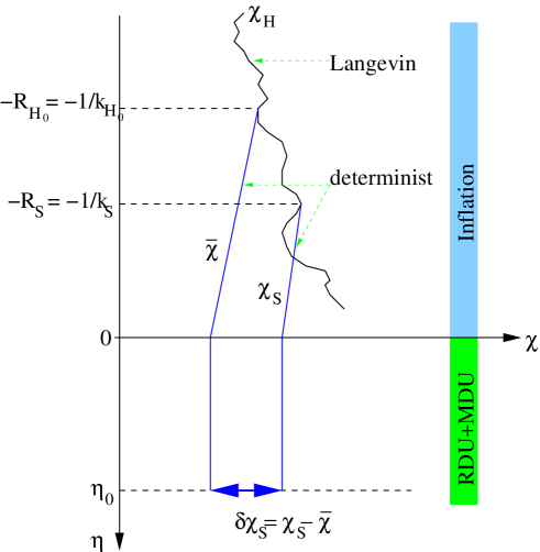
Figure 1: The different filtered quantities and scales entering our problem. $\chi_{{}_{\rm H}}$ follows a stochastic dynamics that can be described by a Langevin equation; it has a time dependent smoothing scale so that more and more modes contribute to the filtered field. The field values ${\bar{\chi}}$ and $\chi_{{}_{\rm S}}$ evolve according a classical Klein-Gordon equation; their smoothing scale is time independent; they coincide with $\chi_{{}_{\rm H}}$ at horizon crossing times.

IV.2 The late time PDF of $\chi_{{}_{\rm H}}(\eta)$.

We follow a formalism first developed to deal with self-interacting fields in a de Sitter background [19] based on the idea that the infrared part of the scalar field may be treated as a classical spacetime dependent stochastic field satisfying a Langevin equation [20, 21] (see Ref. [22] for the case of a massless free field).

Assuming that $\chi$ is slow rolling, the dynamics of $\chi_{{}_{\rm H}}$ can be obtained by averaging Eq. (4) in which both the second time derivative and the Laplacian term can be neglected, since $\chi_{{}_{\rm H}}$ contains only long wavelength modes. Using the identity

$$\dot{\chi}_{{}_{\rm H}}{}_{\bf k}=(\chi_{\bf k})_{R_{\rm H}}{\widehat{W}}(kR_{{}_{\rm H}})-kR_{{}_{\rm H}}\chi_{\bf k}{\widehat{W}}^{\prime}(kR_{{}_{\rm H}})$$ (20)

where ${\widehat{W}}^{\prime}(u)={\rm d}{\widehat{W}}(u)/{\rm d}u$ and where we have used Eq. (5) to express the time derivative of $R_{{}_{\rm H}}$. It follows that

$$\dot{\chi}_{{}_{\rm H}}=-\frac{1}{3H}\bar{V}^{\prime}(\chi_{{}_{\rm H}}+\delta\chi)+\xi_{{}_{\rm Q}}({\bf x},t)$$ (21)

which reduces ($\delta\chi\ll\chi_{{}_{\rm H}}$) to

$$\dot{\chi}_{{}_{\rm H}}=-\frac{1}{3H}\frac{{\rm d}V(\chi_{{}_{\rm H}})}{{\rm d}\chi_{{}_{\rm H}}}+\xi_{{}_{\rm Q}}({\bf x},t).$$ (22)

The term $\xi_{{}_{\rm Q}}({\bf x},t)$ appears from the commutation between $({\dot{\chi}})_{R_{\rm H}}$ and $\dot{\chi}_{{}_{\rm H}}$ using Eq. (20). It is a stochastic noise describing the effects of the small wavelength (quantum) part exiting the horizon on the classical stochastic part. Using Eq. (8), one obtains its expression as

$$\xi_{{}_{\rm Q}}({\bf x},t)=-\int\frac{{\rm d}^{3}{\bf k}}{(2\pi)^{3/2}}(kHR_{{}_{\rm H}})\left[\chi_{k}(t){\widehat{W}}^{\prime}(kR_{{}_{\rm H}})\hbox{e}^{i{\bf k}.{\bf x}}\hat{b}_{\bf k}+\hbox{h.c.}\right].$$ (23)

Indeed, $\xi_{{}_{\rm Q}}$ is quantum noise so that we replace it heuristically by a Gaussian stochastic noise, $\xi$ with a correlator that matches the quantum expectation value in the standard Bunch-Davies vacuum, that is

$$\left<\xi({\bf x},t)\xi({\bf x}^{\prime},t^{\prime}\right>=\left<0\right|\xi_{{}_{\rm Q}}({\bf x},t)\xi_{{}_{\rm Q}}({\bf x}^{\prime},t^{\prime})\left|0\right>.$$ (24)

It follows that

$$\left<\xi({\bf x},t)\xi({\bf x}^{\prime},t^{\prime})\right>=\int\frac{k^{3}{\rm d}k}{4\pi^{2}}\frac{\sin kr}{r}\frac{\chi_{k}(t)\chi_{k}^{*}(t^{\prime})}{a(t)a(t^{\prime})}{\widehat{W}}^{\prime}\left(\frac{k}{a(t)H}\right){\widehat{W}}^{\prime}\left(\frac{k}{a(t^{\prime})H}\right),$$ (25)

with $r\equiv|{\bf x}-{\bf x}^{\prime}|$, which reduces, using the expression (7) on small scales, to [23]

$$\left<\xi({\bf x},t)\xi({\bf x}^{\prime},t^{\prime})\right>=\frac{H^{4}\eta\eta^{\prime}}{4\pi^{2}r}\int{\rm d}k\sin kr(1+ik\eta)(1-ik\eta^{\prime})\hbox{e}^{ik(\eta^{\prime}-\eta)}{\widehat{W}}^{\prime}\left(-k\eta\right){\widehat{W}}^{\prime}\left(-k\eta^{\prime}\right).$$ (26)

Even though $\chi_{{}_{\rm H}}$ remains a quantum operator, it was replaced by a stochastic field in a way that, for all observables, the expectation values of the two fields are in excellent agreement.

In the following and for the sake of simplicity, we consider a window function reducing to a top-hat in Fourier space so that ${\widehat{W}}^{\prime}$ reduces to a Dirac distribution. In that case, using the solution (7) one obtains

$$\left<\xi({\bf x},t)\xi({\bf x}^{\prime},t^{\prime})\right>=\frac{H^{3}}{4\pi^{2}}\frac{\sin a(t)Hr}{a(t)Hr}\delta(t-t^{\prime}).$$ (27)

The case of more realistic window functions (such as a Gaussian) was discussed in Ref. [23].

From a Langevin equation of the form

$$\dot{\chi}_{{}_{\rm H}}=-\beta V^{\prime}+\alpha\xi,\qquad\left<\xi({\bf x},t)\xi({\bf x}^{\prime},t^{\prime})\right>=\delta(t-t^{\prime})$$ (28)

where we assume the two coefficients $\beta$ and $\alpha$ to be independent of $\chi_{{}_{\rm H}}$, one can deduce [24] a equation, the Fokker-Planck equation, for the PDF of $\chi_{{}_{\rm H}}$ of the form

$$\partial_{t}{\cal P}=\beta\partial^{2}_{\chi_{{}_{\rm H}}}{\cal P}+\frac{\alpha}{2}\partial_{\chi_{{}_{\rm H}}}[V^{\prime}{\cal P}].$$ (29)

It follows from the Langevin equation (22) with a top-hat window function for which the noise is given by Eq. (27) with $\beta=-1/3H$ and $\alpha=H^{3/2}/2\pi$ that the one-point PDF, ${\cal P}(\chi_{{}_{\rm H}},t)$, is solution of

$$\partial_{t}{\cal P}=\frac{H^{3}}{8\pi^{2}}\partial_{\chi_{{}_{\rm H}}}^{2}{\cal P}+\frac{1}{3H}\partial_{\chi_{{}_{\rm H}}}\left(V^{\prime}{\cal P}\right).$$ (30)

In a cosmological context, this equation was first derived in Ref. [19] in the case $H={\rm const.}$, which we are interested in, and then in Ref. [22] in the case $V^{\prime}=0$. It was generalized to more involved situations in Ref. [25].

The solution of Eq. (30) where studied in Ref. [21] in which it is shown that ${\cal P}$ approaches the static equilibrium solution

$${\cal P}_{{}_{\rm eq}}={\cal N}^{-1}\exp\left(-\frac{8\pi^{2}}{3H^{4}}V(\chi_{{}_{\rm H}})\right),\qquad{\cal N}\equiv\int_{-\infty}^{\infty}\exp\left(-\frac{8\pi^{2}}{3H^{4}}V(\chi_{{}_{\rm H}})\right){\rm d}\chi_{{}_{\rm H}}$$ (31)

irrespectively of the initial conditions.

For the quartic potential, Eq. (3), we find

$${\cal P}_{{}_{\rm eq}}(\chi_{{}_{\rm H}})=\frac{1}{2\Gamma(5/4)H}\left(\frac{\pi^{2}\lambda}{9}\right)^{1/4}\exp\left[-\frac{\pi^{2}\lambda}{9H^{4}}\chi_{{}_{\rm H}}^{4}\right].$$ (32)

They are few lessons to learn from this result. The excursion values of $\chi_{{}_{\rm H}}$ are bounded. Their distribution does not depend on the remote past history of $\chi$ and, importantly for the following, the typical value one can expect for $\chi_{{}_{\rm H}}$, and therefore ${\bar{\chi}}$, is $H/\lambda^{1/4}$.

IV.3 Consequences on the shape of the PDF of $\delta\chi_{{}_{\rm S}}$

We can then insights into the shape of the probability distribution function of $\delta\chi_{{}_{\rm S}}$ as a function of ${\bar{\chi}}$.

Quantitative results can be drawn from the perturbation approach we initially developed in our previous work [10]. We expand the filtered field in terms of the coupling constant as

$$\chi_{{}_{\rm S}}(\eta)=\chi_{{}_{\rm S}}^{(0)}(\eta)+\chi_{{}_{\rm S}}^{(1)}(\eta)+\dots.$$ (33)

$\chi_{{}_{\rm S}}^{(0)}$ represents the value of the filtered field when the interaction term is switched off. In the slow-roll regime the field $\chi_{{}_{\rm S}}$ follows the Klein-Gordon equation (22). Contrary of the previously studied case of $\chi_{{}_{\rm H}}$, the evolution equation does not contain any noise term because the smoothing scale $R$ is now fixed and there is no new modes entering $\chi_{{}_{\rm S}}$. The free filtered field, $\chi_{{}_{\rm S}}^{(0)}$, is therefore constant and, from the discussion of the previous section, it cannot be assumed to be Gaussian distributed with a zero mean: its expectation value, ${\overline{\chi_{{}_{\rm S}}^{(0)}}}$, is actually the value of ${\bar{\chi}}$ at time $\eta=1/R_{{}_{\rm H}}$. Since this field value is going to be only weakly affected but its subsequent evolution, in the following we will identify ${\overline{\chi_{{}_{\rm S}}^{(0)}}}$ and ${\bar{\chi}}$. The difference $\delta\chi_{{}_{\rm S}}^{(0)}\equiv\chi_{{}_{\rm S}}^{(0)}-{\overline{\chi_{{}_{\rm S}}^{(0)}}}$ has been built up from the modes that have left the horizon between $-1/k_{{}_{\rm H}}$ and $-1/k_{{}_{\rm S}}$. It can be assumed to be Gaussian distributed with a width precisely given by $\sigma_{\delta}$.

The first order term in $\lambda$, ${\chi_{{}_{\rm S}}}^{(1)}$, evolves according to

$$3H\dot{\chi_{{}_{\rm S}}}^{(1)}=-\frac{\lambda}{3!}\left[\chi_{{}_{\rm S}}^{(0)}\right]^{3}.$$ (34)

In this approach the treatment of the filtering of the r.h.s. of this equation is very crude. The results we are going to find can anyway be checked against more rigorous calculations based on the computed shape of the tri-spectrum. Our goal now is to capture the essential effects of a non-vanishing ${\bar{\chi}}$ on the statistical properties of $\delta\chi_{{}_{\rm S}}$.

The equation of evolution (34) can be solved to get

$$\chi_{{}_{\rm S}}^{(1)}(t)=-\lambda(t-t_{{}_{\rm H}})\frac{\left(\chi_{{}_{\rm S}}^{(0)}\right)^{3}}{18\,H},$$ (35)

which also reads

$$\chi_{{}_{\rm S}}^{(1)}(t)=-\frac{\lambda N_{e}}{18\,H^{2}}\left(\chi_{{}_{\rm S}}^{(0)}\right)^{3},$$ (36)

$N_{e}$ being the number of $e$-fold between $t_{H}$ and the end of inflation.

These results imply that

$${\bar{\chi}}\approx{\overline{\chi_{{}_{\rm S}}^{(0)}}}-\frac{\lambda N_{e}}{18\,H^{2}}\left[\left({\overline{\chi_{{}_{\rm S}}^{(0)}}}\right)^{3}+3\,{\overline{\chi_{{}_{\rm S}}^{(0)}}}\,\sigma_{\delta}^{2}\right]$$ (37)

which explicitly shows that ${\bar{\chi}}$ and ${\overline{\chi_{{}_{\rm S}}^{(0)}}}$ are equal at leading order in $\lambda$. It also gives

$$\delta\chi_{{}_{\rm S}}=\delta\chi_{{}_{\rm S}}^{(0)}-\frac{\lambda N_{e}}{18\,H^{2}}\left\{\left(\delta\chi_{{}_{\rm S}}^{(0)}\right)^{3}+3\left[\left(\delta\chi_{{}_{\rm S}}^{(0)}\right]^{2}-\sigma_{\delta}^{2}\right){\bar{\chi}}+3\delta\chi_{{}_{\rm S}}^{(0)}{\bar{\chi}}^{2}\right\}.$$ (38)

It is straightforward to see that $\delta\chi_{{}_{\rm S}}$ has acquired a non zero third order moment,

$$\overline{\delta\chi_{{}_{\rm S}}^{3}}=-\frac{\lambda N_{e}}{H^{2}}{\bar{\chi}}\sigma_{\delta}^{4}$$ (39)

at leading order in $\lambda$. This is a finite volume effect in the sense that it exists for a fixed (not ensemble averaged) value of ${\bar{\chi}}$. This effect cannot a priori be neglected. From the study of the previous paragraph, we know that ${\bar{\chi}}$ should be of the order of $H/\lambda^{1/4}$, which implies that the reduced skewness of $\delta\chi_{{}_{\rm S}}$, $\overline{\delta}\chi_{{}_{\rm S}}^{3}/(\overline{\delta}\chi_{{}_{\rm S}}^{2})^{3/2}\sim\lambda^{3/4}N_{e}\sigma_{\delta}/H$ is significant as soon as $\lambda^{3/4}N_{e}$ approaches unity, a condition similar to that encountered in Sect. III.2.

Actually the evolution equation for $\chi_{{}_{\rm S}}$ can be solved in

$$\chi_{{}_{\rm S}}=\frac{\chi_{{}_{\rm S}}^{(0)}}{\sqrt{1-\frac{\lambda\,N_{e}}{9H^{2}}\left(\chi_{{}_{\rm S}}^{(0)}\right)^{2}}}$$ (40)

and the distribution of $\chi_{{}_{\rm S}}$ can then be infered from that of $\chi_{{}_{\rm S}}^{(0)}$ assuming the latter is Gaussian distributed with a non-zero mean value .

Figure 2: PDF of $\delta\chi_{{}_{\rm S}}=\delta\chi_{{}_{\rm S}}-{\bar{\chi}}$ for different values of ${\bar{\chi}}$. The dashed line corresponds to a Gaussian distribution; the dot-dashed line to the deformed distribution of $\delta\chi_{{}_{\rm S}}$ when $\lambda N_{e}/H^{2}=1$ and ${\bar{\chi}}=0$ and the solid lines when the latter equals $0.5$ and $1$.

In figure 2, we present the deformation of the PDF of $\delta\chi_{{}_{\rm S}}$ while ${\bar{\chi}}$ is varied. As expected, it shows that when ${\bar{\chi}}$ is not zero, the PDF gets skewed in a way that can be easily understood: when ${\bar{\chi}}$ is positive it gets more difficult to have excursion towards larger value of $\chi_{{}_{\rm S}}$, but easier to roll down to smaller values. It is as if the field $\chi$ was actually evolving in the potential $\lambda(\chi+{\bar{\chi}})/4!$. As a result one naturally expects the field $\chi$ to have non-vanishing three-point function. As mentioned before, these calculations treat the smoothing in a rather simplified way but we think that for illustrative purposes it encapsulates the main effects that we want to describe.

It nonetheless shows the way for the computation of the finite volume effects for expected stochastic properties of the field.

V Finite volume effects on high order cumulants

What the Langevin picture suggests is that finite volume effects on the observed quantities are not due to the whole stochastic process that give birth the observed field but mainly to the value of ${\bar{\chi}}$ alone. In other words, we expect to have

$${\cal P}(X_{n})=\int{\cal P}({\bar{\chi}})\,\delta\left(X_{n}-\left<\left(\chi_{{}_{\rm S}}-{\bar{\chi}}\right)^{n}\right>_{{\bar{\chi}}}\right)\,{\rm d}{\bar{\chi}}.$$ (41)

This form (41) implies in particular that the PDF of $X_{n}$, ${\cal P}(X_{n})$, is expected to be peaked around the expectation value of $\delta\chi_{{}_{\rm S}}^{n}$ at ${\bar{\chi}}$ fixed. In particular, it implies that

$$\left<X_{n}^{p}\right>\simeq\left<\left(\left<\delta\chi_{{}_{\rm S}}^{n}\right>_{{\bar{\chi}}}\right)^{p}\right>$$ (42)

We will explicitly check such a property for the lower order cumulants.

In general, for small enough values of ${\bar{\chi}}$, the constrained ensemble averages of the form $\left<A(\chi)\right>_{{\bar{\chi}}}$ should be given by

$$\left<A(\chi)\right>_{{\bar{\chi}}}\simeq\left<A(\chi){\bar{\chi}}\right>\,\frac{{\bar{\chi}}}{\sigma^{2}_{{\bar{\chi}}}}$$ (43)

where $\sigma^{2}_{{\bar{\chi}}}$ is the variance square of the ${\bar{\chi}}$ fluctuations. This relation, exact for Gaussian fields, is only approximate in general. It can be derived for stochastic variables following a quasi-Gaussian distribution. Here, it will be valid only if the excursion values of ${\bar{\chi}}$ are modest compared to the fluctuations of $\delta\chi_{{}_{\rm S}}$.

Not surprisingly, it implies that the even order cumulants are left unchanged.

V.1 The bi-spectrum

Non trivial finite volume effects are then going to appear at the level of the third order cumulants or correlation functions. In particular it induces a non-vanishing bispectrum, three-point correlation function of the wave-vectors, which is going to be given by

$$\left<\chi({\bf k}_{1})\chi({\bf k}_{2})\chi({\bf k}_{3})\right>_{{\bar{\chi}}}\simeq\left<\chi({\bf k}_{1})\chi({\bf k}_{2})\chi({\bf k}_{3}){\bar{\chi}}\right>_{c}\ \frac{{\bar{\chi}}}{\sigma_{{\bar{\chi}}}^{2}}$$ (44)

when ${\bar{\chi}}$ is small enough. Using Eq. (10) to express $\left<\chi_{{\bf k}_{1}}\ldots\chi_{{\bf k}_{4}}\right>_{c}$ and using that Eq. (2) implies that ${\bar{\chi}}_{\bf k}=\chi_{\bf k}\widehat{W}(kR_{{}_{\rm H}})$, the previous expression reduces to

$$\left<\chi({\bf k}_{1})\chi({\bf k}_{2})\chi({\bf k}_{3})\right>_{{\bar{\chi}}} = -\frac{\lambda}{3H^{2}}(2\pi)^{9/2}\,\frac{{\bar{\chi}}}{\sigma_{{\bar{\chi}}}^{2}}\,\log\left[\left(\sum_{i}k_{i}+\left|\sum_{i}{\bf k}_{i}\right|\right)\eta\right]\times$$ (45)

$$\left\{P(k_{1})P(k_{2})P(k_{3})+P\left(\left|\sum_{i}{\bf k}_{i}\right|\right)\left[P(k_{1})P(k_{2})+\hbox{perm.}\right]\right\}\widehat{W}\left(\left|\sum_{i}{\bf k}_{i}\right|R_{{}_{\rm H}}\right).$$

The factor $\widehat{W}\left(|{\bf k}_{1}+\ldots{\bf k}_{3}|R_{{}_{\rm H}}\right)$, that arises from the contribution of modes with $k<1/R_{{}_{\rm H}}$ to ${\bar{\chi}}$, ensures that $|{\bf k}_{1}+\ldots{\bf k}_{3}|$ is small compared to each of the $k_{i}$, and thus can be neglected in the log term. It implies that for an Harrison-Zel’dovich type spectrum that $P(|{\bf k}_{1}+\ldots+{\bf k}_{3}|)\gg P(k_{i})$ so that the first term of (45) is negligible. As a result we deduce that

$$\left<\chi({\bf k}_{1})\chi({\bf k}_{2})\chi({\bf k}_{3})\right>_{{\bar{\chi}}}\simeq-\frac{\lambda{\bar{\chi}}}{3H^{2}}(2\pi)^{9/2}\log\left[\left(\sum_{i}k_{i}\right)\eta\right]\left[P(k_{1})P(k_{2})+\hbox{perm.}\right]\frac{P\left(\left|\sum_{i}{\bf k}_{i}\right|\right)\widehat{W}\left(\left|\sum_{i}{\bf k}_{i}\right|R_{{}_{\rm H}}\right)}{\sigma_{{\bar{\chi}}}^{2}}.$$ (46)

Now, noting that, by definition, $P(k)\widehat{W}(kR_{{}_{\rm H}}){\rm d}^{3}{\bf k}/\sigma_{{\bar{\chi}}}^{2}$ integrates to unity and that the function ${P\left(\left|\sum_{i}{\bf k}_{i}\right|\right)\widehat{W}\left(\left|\sum_{i}{\bf k}_{i}\right|R_{{}_{\rm H}}\right)}$ is, for the modes we are interested in, peaked near the origin we obtain that this factor is essentially equal to $\delta\left(\sum_{i}{\bf k}_{i}\right)$. It therefore implies that

$$\left<\chi({\bf k}_{1})\chi({\bf k}_{2})\chi({\bf k}_{3})\right>_{{\bar{\chi}}}=-\frac{\lambda{\bar{\chi}}}{3H^{2}}(2\pi)^{9/2}\,\log\left[\left(\sum_{i}k_{i}\right)\eta\right]\,\left[P(k_{1})P(k_{2})+\hbox{perm.}\right]\,\delta\left(\sum_{i}{\bf k}_{i}\right).$$ (47)

Here is one of the main points of this paper: Finite volume effects induce a non-vanishing three-point function although the potential in which $\chi$ evolves is symmetric.

From this bispectrum it is possible to compute the third order moment of $\delta\chi_{{}_{\rm S}}$. Its amplitude will be in agreement with what had been obtained from the Langevin equation. It is also the three-point function one expects for a field evolving in potential $\lambda\,{\bar{\chi}}\,\chi/3!$ (see Ref. [26] for details).

V.2 The three-point cumulant

We now turn to the lowest order cumulant exhibiting a non-trivial result due to a non-vanishing ${\bar{\chi}}$, that is $X_{3}$, which reads

$$X_{3}=\int\frac{{\rm d}^{3}{\bf k}_{1}\ldots{\rm d}^{3}{\bf k}_{3}}{(2\pi)^{9/2}}\widehat{W}(|{\bf k}_{1}+{\bf k}_{2}+{\bf k}_{3}|R_{{}_{\rm H}})\widetilde{W}(k_{1})\widetilde{W}(k_{2})\widetilde{W}(k_{3})\chi_{{\bf k}_{1}}\chi_{{\bf k}_{2}}\chi_{{\bf k}_{3}}.$$ (48)

Obviously its ensemble average vanishes,

$$\left<X_{3}\right>=0$$

but not $\left<X_{3}^{2}\right>_{c}$. Let us check, as expected from our analysis [see Eqs. (41-42)], that it is well approximated by $\left<\left(\left<X_{3}\right>_{{\bar{\chi}}}\right)^{2}\right>$.

To evaluate the latter expression, we start from the expression of $\left<X_{3}\right>_{{\bar{\chi}}}$ that is defined by

$$\left<X_{3}\right>_{{\bar{\chi}}}\simeq\frac{{\bar{\chi}}}{\sigma_{{\bar{\chi}}}^{2}}\int\frac{{\rm d}^{3}{\bf k}_{1}\ldots{\rm d}^{3}{\bf k}_{3}}{(2\pi)^{9/2}}\widehat{W}(|{\bf k}_{1}+\ldots+{\bf k}_{3}|R_{{}_{\rm H}})\widetilde{W}(k_{1})\ldots\widetilde{W}(k_{3})\left<\chi_{{\bf k}_{1}}\ldots\chi_{{\bf k}_{3}}\right>_{{\bar{\chi}}}.$$ (49)

Using Eq. (47), it reduces after integration over ${\bf k}_{3}$ to

$$\left<X_{3}\right>_{{\bar{\chi}}}\simeq-\frac{\lambda{\bar{\chi}}}{3H^{2}}\int{\rm d}^{3}{\bf k}_{1}{\rm d}^{3}{\bf k}_{2}\widetilde{W}(k_{1})\widetilde{W}(k_{2})\widetilde{W}(|{\bf k}_{1}+{\bf k}_{2}|)\left\{P(k_{1})P(k_{2})+P(|{\bf k}_{1}+{\bf k}_{2}|)\left[P(k_{1})+P(k_{2})\right]\right\}$$ (50)

where the window function $\widehat{W}(|{\bf k}_{1}+\ldots+{\bf k}_{3}|R_{{}_{\rm H}})$ was aborbed during the integration over ${\bf k}_{3}$ due to the Dirac distribution. Such an expression can be computed following the same lines as for the computation of the expectation value of the fourth order cumulant (17),

$$\left<X_{3}\right>_{{\bar{\chi}}}\simeq-{\lambda{\bar{\chi}}\over 3H^{2}}\left(\frac{H^{2}}{2}\right)^{2}\int_{k_{{}_{\rm H}}}^{k_{{}_{\rm S}}}{{\rm d}^{3}{\bf k}_{1}\over k_{1}^{3}}\int_{k_{{}_{\rm H}}}^{k_{{}_{\rm S}}}{{\rm d}^{3}{\bf k}_{2}\over k_{2}^{3}}\ 3{\widetilde{W}}\left(|{\bf k}_{1}+{\bf k}_{2}|\right)\ \log\left[\left(k_{1}+k_{2}+|{\bf k}_{1}+{\bf k}_{2}|\right)\eta\right].$$ (51)

where, again, ${\widetilde{W}}\left(|{\bf k}_{1}+{\bf k}_{2}|\right)$ simply expresses the conditions, $k_{{}_{\rm H}}<|{\bf k}_{1}+{\bf k}_{2}|<k_{{}_{\rm S}}$. A simple expression for this integral can be obtained when $k_{{}_{\rm S}}$ is much larger than $k_{{}_{\rm H}}$ where it is possible to replace ${\bf k}_{1}+{\bf k}_{2}$ and $k_{1}+k_{2}+|{\bf k}_{1}+{\bf k}_{2}|$ by respectively either ${\bf k}_{1}$ and $2\,k_{1}$ or ${\bf k}_{2}$ and $2\,k_{2}$. Finally the integral reads,

$$\left<X_{3}\right>_{{\bar{\chi}}}=-\lambda\,{\bar{\chi}}(4\pi)^{2}\left(\frac{H^{2}}{2}\right)^{2}\log^{2}\left({k_{{}_{\rm S}}\over k_{{}_{\rm H}}}\right)\log\left(2\eta k_{{}_{\rm S}}^{2/3}k_{{}_{\rm H}}^{1/3}\right)$$ (52)

e.g.

$$\left<X_{3}\right>_{{\bar{\chi}}}=-{\lambda\ {\bar{\chi}}\ \log\left(2\eta k_{{}_{\rm S}}^{2/3}k_{{}_{\rm H}}^{1/3}\right)}\frac{\sigma_{\delta}^{4}}{H^{2}}$$ (53)

which reproduces the result (39) if $N_{e}$ is identified with $\log\left(2\eta k_{{}_{\rm S}}^{2/3}k_{{}_{\rm H}}^{1/3}\right)$. In conclusion, we end up with

$$\left<\left(\left<X_{3}\right>_{{\bar{\chi}}}\right)^{2}\right>^{1/2}\simeq{\lambda\ \log\left(2\eta k_{{}_{\rm S}}^{2/3}k_{{}_{\rm H}}^{1/3}\right)}\frac{\sigma_{\delta}^{4}\sigma_{{\bar{\chi}}}}{H^{2}}$$ (54)

In this case, it is actually possible to compute $\left<X_{3}^{2}\right>$ from a perturbation theory approach in order to check that its dominant contribution is indeed $\left<\left(\left<X_{3}\right>_{{\bar{\chi}}}\right)^{2}\right>$. $\left<X_{3}^{2}\right>$ is given in general by

$$\left<X_{3}^{2}\right> = \int\frac{{\rm d}^{3}{\bf k}_{1}\ldots{\rm d}^{3}{\bf k}_{3}}{(2\pi)^{9/2}}\int\frac{{\rm d}^{3}{\bf k}^{\prime}_{1}\ldots{\rm d}^{3}{\bf k}^{\prime}_{3}}{(2\pi)^{9/2}}\widetilde{W}(k_{1})\ldots\widetilde{W}(k_{3})\widetilde{W}(k^{\prime}_{1})\ldots\widetilde{W}(k^{\prime}_{3})$$ (55)

$$\qquad\widehat{W}(|{\bf k}_{1}+\ldots+{\bf k}_{3}|R_{{}_{\rm H}})\widehat{W}(|{\bf k}^{\prime}_{1}+\ldots+{\bf k}^{\prime}_{3}|R_{{}_{\rm H}})\left<\chi_{{\bf k}_{1}}\ldots\chi_{{\bf k}_{3}}\chi_{{\bf k}^{\prime}_{1}}\ldots\chi_{{\bf k}^{\prime}_{3}}\right>_{c}.$$

It involves the expression of the 6-point correlation function $\left<\chi_{{\bf k}_{1}}\ldots\chi_{{\bf k}_{3}}\chi_{{\bf k}^{\prime}_{1}}\ldots\chi_{{\bf k}^{\prime}_{3}}\right>_{c}$ which, in a perturbation theory approach, can be split into 2 contributions

$$I\equiv\left<\chi^{(0)}_{{\bf k}_{1}}\chi^{(0)}_{{\bf k}_{2}}\chi^{(1)}_{{\bf k}_{3}}\chi^{(0)}_{{\bf k}^{\prime}_{1}}\chi^{(0)}_{{\bf k}^{\prime}_{2}}\chi^{(1)}_{{\bf k}^{\prime}_{3}}\right>,\qquad II\equiv\left<\chi^{(0)}_{{\bf k}_{1}}\chi^{(0)}_{{\bf k}_{2}}\chi^{(2)}_{{\bf k}_{3}}\chi^{(0)}_{{\bf k}^{\prime}_{1}}\chi^{(0)}_{{\bf k}^{\prime}_{2}}\chi^{(0)}_{{\bf k}^{\prime}_{3}}\right>$$

where

$$\chi^{(1)}({\bf x})\sim-\frac{\lambda}{18}\frac{N_{e}}{H^{2}}\left[\chi^{(0)}({\bf x})\right]^{3},\qquad\chi^{(2)}({\bf x})\sim\frac{\lambda^{2}}{8}\frac{N_{e}^{2}}{H^{4}}\left[\chi^{(0)}({\bf x})\right]^{5}.$$

This implies that

$$I=(2\pi)^{9}\frac{\lambda^{2}}{18^{2}}18^{2}\frac{N_{e}^{2}}{H^{4}}P(k_{1})P(k_{2})P({\bf k}_{3}+{\bf k}_{1}+{\bf k}_{2}|)P(k_{2}^{\prime})P(k^{\prime}_{3})\,\delta\left(\sum{\bf k}_{i}+\sum{\bf k}^{\prime}_{i}\right).$$ (56)

and

$$II=(2\pi)^{9}\frac{\lambda^{2}}{8}\,6!\,\frac{N_{e}^{2}}{H^{4}}P(k_{1})P(k_{2})P(k_{1}^{\prime})P(k_{2}^{\prime})P(k^{\prime}_{3})\,\delta\left(\sum{\bf k}_{i}+\sum{\bf k}^{\prime}_{i}\right)$$ (57)

where $18^{2}$ and $6!$ are symmetry factors.

Let us evaluate the first contribution

$$\left<X_{3}^{2}\right>_{c}^{(I)} = \lambda^{2}\frac{N_{e}^{2}}{H^{4}}\int{\rm d}^{3}{\bf k}_{1}{\rm d}^{3}{\bf k}_{2}P(k_{1})P(k_{2})\widetilde{W}(k_{1})\widetilde{W}(k_{2})\int{\rm d}^{3}{\bf k}_{3}P(|{\bf k}_{3}+{\bf k}_{1}+{\bf k}_{2}|)\widetilde{W}(k_{3})\widehat{W}^{2}(|{\bf k}_{1}+{\bf k}_{2}+{\bf k}_{3}|R_{{}_{\rm H}})$$ (58)

$$\int{\rm d}^{3}{\bf k}^{\prime}_{1}{\rm d}^{3}{\bf k}^{\prime}_{2}P(k^{\prime}_{1})P(k^{\prime}_{2})\widetilde{W}(k^{\prime}_{1})\widetilde{W}(k^{\prime}_{2})\widetilde{W}(|{\bf k}_{1}+{\bf k}_{2}+{\bf k}_{3}+{\bf k}^{\prime}_{1}+{\bf k}^{\prime}_{2}|.$$

The term $\widehat{W}^{2}(|{\bf k}_{1}+{\bf k}_{2}+{\bf k}_{3}|R_{{}_{\rm H}})$ implies that $|{\bf k}_{1}+{\bf k}_{2}+{\bf k}_{3}|\ll R_{{}_{\rm H}}$ so that $\widetilde{W}(k_{3})\sim\widetilde{W}(|{\bf k}_{1}+{\bf k}_{2}|)$ and $\widetilde{W}(|{\bf k}_{1}+{\bf k}_{2}+{\bf k}_{3}+{\bf k}^{\prime}_{1}+{\bf k}^{\prime}_{2}|\sim\widetilde{W}(|{\bf k}^{\prime}_{1}+{\bf k}^{\prime}_{2}|)$. Setting ${\bf e}={\bf k}_{1}+{\bf k}_{2}+{\bf k}_{3}$, we conclude that

$$\left<X_{3}^{2}\right>_{c}^{(I)} \sim \lambda^{2}\frac{N_{e}^{2}}{H^{4}}\left[\int{\rm d}^{3}{\bf k}_{1}{\rm d}^{3}{\bf k}_{2}P(k_{1})P(k_{2})\widetilde{W}(k_{1})\widetilde{W}(k_{2})\widetilde{W}(|{\bf k}_{1}+{\bf k}_{2}|)\right]^{2}\,\int{\rm d}^{3}{\bf e}P(e)\widehat{W}^{2}(eR_{{}_{\rm H}}).$$ (59)

The integral over ${\bf e}$ reduces to $\sigma_{{\bar{\chi}}}^{2}$ so that

$$\left<X_{3}^{2}\right>_{c}^{(I)} \sim \lambda^{2}\frac{N_{e}^{2}}{H^{4}}\,\sigma_{{\bar{\chi}}}^{2}\left[\int{\rm d}^{3}{\bf k}_{1}{\rm d}^{3}{\bf k}_{2}P(k_{1})P(k_{2})\widetilde{W}(k_{1})\widetilde{W}(k_{2})\widetilde{W}(|{\bf k}_{1}+{\bf k}_{2}|)\right]^{2}.$$ (60)

The second contribution reduces to

$$\left<X_{3}^{2}\right>_{c}^{(II)} \sim 90\lambda^{2}\frac{N_{e}^{2}}{H^{4}}\int{\rm d}^{3}{\bf k}_{1}{\rm d}^{3}{\bf k}_{2}P(k_{1})P(k_{2})\widetilde{W}(k_{1})\widetilde{W}(k_{2})\widetilde{W}(|{\bf k}_{1}+{\bf k}_{2}|)$$ (61)

$$\int{\rm d}^{3}{\bf k}^{\prime}_{1}{\rm d}^{3}{\bf k}^{\prime}_{2}{\rm d}^{3}{\bf k}^{\prime}_{3}P(k_{1}^{\prime})P(k_{2}^{\prime})P(k_{3}^{\prime})\widetilde{W}(k_{1}^{\prime})\widetilde{W}(k_{2}^{\prime})\widetilde{W}(k_{3}^{\prime})\widehat{W}^{2}(|{\bf k}^{\prime}_{1}+{\bf k}^{\prime}_{2}+{\bf k}^{\prime}_{3}|R_{{}_{\rm H}}).$$

The second integral reduces to

$$\int{\rm d}^{3}{\bf k}^{\prime}_{1}{\rm d}^{3}{\bf k}^{\prime}_{2}{\rm d}^{3}P(k_{1}^{\prime})P(k_{2}^{\prime})P(|{\bf k}^{\prime}_{1}+{\bf k}^{\prime}_{2}|)\widetilde{W}(k_{1}^{\prime})\widetilde{W}(k_{2}^{\prime})\widetilde{W}(|{\bf k}^{\prime}_{1}+{\bf k}^{\prime}_{2}|)\int{\rm d}^{3}{\bf e}\widehat{W}^{2}(eR_{{}_{\rm H}}).$$

The integral over ${\bf e}$ gives $\sim R_{{}_{\rm H}}^{-3}$ so that

$$\left<X_{3}^{2}\right>_{c}^{(II)} \sim 90\lambda^{2}\frac{N_{e}^{2}}{H^{4}}R_{{}_{\rm H}}^{-3}\int{\rm d}^{3}{\bf k}_{1}{\rm d}^{3}{\bf k}_{2}P(k_{1})P(k_{2})\widetilde{W}(k_{1})\widetilde{W}(k_{2})\widetilde{W}(|{\bf k}_{1}+{\bf k}_{2}|)$$ (62)

$$\int{\rm d}^{3}{\bf k}^{\prime}_{1}{\rm d}^{3}{\bf k}^{\prime}_{2}P(k_{1}^{\prime})P(k_{2}^{\prime})P(|{\bf k}^{\prime}_{1}+{\bf k}^{\prime}_{2}|)\widetilde{W}(k_{1}^{\prime})\widetilde{W}(k_{2}^{\prime})\widetilde{W}(|{\bf k}^{\prime}_{1}+{\bf k}^{\prime}_{2}|).$$

Due to the term $\widetilde{W}(|{\bf k}^{\prime}_{1}+{\bf k}^{\prime}_{2}|)$, we deduce that, in the case of a Harrisson-Zel’dovich spectrum, $(R_{{}_{\rm S}}/R_{{}_{\rm H}})^{3}<|{\bf k}^{\prime}_{1}+{\bf k}^{\prime}_{2}|^{-3}R_{{}_{\rm H}}^{-3}<1$ so that this contribution is at most equal to the one of Eq. (60). As a result we have

$$\left<X_{3}^{2}\right>\simeq\left<X_{3}^{2}\right>_{c}^{(I)}.$$ (63)

From Eq. (60), this reduces to

$$\left<X_{3}^{2}\right>^{1/2}\simeq\lambda\,N_{e}(2\pi)^{3}\frac{\sigma_{\delta}^{4}\sigma_{{\bar{\chi}}}}{H^{2}}$$ (64)

that can be identified with the expectation value of $\left<\delta\chi_{{}_{\rm S}}^{3}\right>_{{\bar{\chi}}}^{2}$ over the distribution of ${\bar{\chi}}$, as obtained in Eq. (54).

This explicit computation shows that, as expected, the fluctuations of the measured values of $X_{3}$ are mainly due the fluctuations of ${\bar{\chi}}$. It justifies for instance that one should expect to see a bispectrum of the form (47) for such inflationary models.

VI Conclusions

In this article we have focused on the phenomenology of the non-Gaussianity generated in models developed in Refs. [10, 17]. Interestingly, whereas the metric perturbation statistics involve only two microscopic parameters respectively related to the weight of the non-Gaussian component and to its PDF, the finite volume effects imply that the statistical properties of any observational quantity will involve a third parameter. This new parameter arises from the fact that the mean value, ${\bar{\chi}}$, of the field on the size of the observable universe does not vanish a priori. Obviously ${\bar{\chi}}$ cannot be determined on the basis of any observation. As described in § IV, it implies that the originally symmetric PDF can be skewed and that this skewness is directly proportional to ${\bar{\chi}}$ that needs to be considered as a new parameter of the PDF while dealing with observations.

These results open the way for more detailed phenomenological studies. To see how those properties translate for the temperature and local density fields is not easy. Such investigation will probably require numerical tools such that developed in Ref. [27].

Acknowledgements: We thank Nabila Aghanim and Tristan Brunier for discussions as well as Alain Riazuelo for early discussions on the project.

References

-
[1]
A. Kogut et al., Astrophys. J. 464 (1996) 29;
N. Aghanim, O. Forni, and F.R. Bouchet, Astron. Astroph. 365 (2001) 341;
E. Komatsu, and D.N. Spergel, Phys. Rev. D 63 (2001) 0633002. -
[2]
C.G. Park et al., Astrophys. J. 556 (2001) 582;
S.F. Shandarin et al., Astroph. J. Suppl. 141 (2002) 1. -
[3]
J.H.P. Wu et al., Phys. Rev. Lett. 87 (2001)
251303;
M.G. Santos et al., Phys. Rev. Lett. 88 (2002) 241302;
G. Polenta et al., Astrophys. J. 572 (2002) L27. -
[4]
F. Bernardeau, Y. Mellier, and L. van Waerbeke, Astron. Astrophys. 389 (2002) L28;
M. Takada and B. Jain, Mon. Not. Roy. Astron. Soc. 337 (2002) 875;
R. Durrer et al., Phys. Rev. D 62 (2000) 021301(R). - [5] E. Komatsu et al., Astrophys. J. Suppl. 148 (2003) 119.
- [6] W.N. Colley and J.R. Gott III, Mon. Not. Roy. Astron. Soc. 344 (2003) 686.
-
[7]
E. Gaztañaga and J. Wagg, Phys. Rev. D 68 (2003) 021302;
E. Gaztañaga et al., Mon. Not. Roy. Astron. Soc. 346 (2003) 47. - [8] C.G. Park, [arXiv:astro-ph/0307469].
-
[9]
V. Mukhanov and G.V. Chibisov, JETP Lett. 33 (1981) 532;
A.D. Linde, Particle physics and inflationary cosmology, Harwood (Chur, Witzerland, 1990);
J. Maldacena, JHEP 0305 (2003) 013. - [10] F. Bernardeau and J.-P. Uzan, Phys. Rev. D 66 (2002) 103506.
- [11] A.A. Starobinsky, Grav. Cosm. 4 (1998) 88.
-
[12]
T.J. Allen, B. Grinstein, and M.B. Wise, Phys. Lett. B 197
(1987) 66;
P.J.E. Peebles, Astrophys. J. 483 (1999) L1. - [13] E. Copeland, J.E. Lidsey, and D. Wands, Phys. Lett. B 443 (1998) 97.
-
[14]
A. Gangui and S. Mollerach, Phys. Rev. D 54 (1996) 4750;
R. Durrer, M. Kunz, and A. Melchiorri, Phys. Rept. 364 (2002). -
[15]
D. Lyth and D. Wands, Phys. Lett. B 524 (2002) 5;
D. Lyth, C. Ungarelli, and D. Wands, Phys. Rev. D 67 (2003) 023509;
N. Bartolo, S. Matarrese, and A. Riotto, [arXiv:hep-ph/0309033]. - [16] M. Zaldariagga, [arXiv:astro-ph/0306006]
- [17] F. Bernardeau and J.-P. Uzan, Phys. Rev. D 67 (2003) 121301(R).
- [18] F. Bernardeau et al., Phys. Rept. 367 (2002) 1.
- [19] A.A. Starobinsky, Phys. Lett. B 117 (1982) 175.
- [20] A.A. Starobinsky, in Current topics in field theory, quantum gravity and strings, Eds. H. De Vega and N. Sanchez, Lecture Notes in Physics 246(Springer, Heidelberg, 1986) p. 107.
- [21] A.A. Starobinsky and J. Yokoyama, Phys. Rev. D 50 (1994) 6357.
- [22] A. Vilenkin, Phys. Rev. D 27 (1983) 2848.
- [23] S. Winitzki and A. Vilenkin, Phys. Rev. D 61 (2000) 084008.
- [24] S. Chandrasekhar, Rev. Mod. Phys. 15 (1943) 1.
- [25] A.D. Linde, D.A. Linde, and A. Mezhlumian, Phys. Rev. D 49 (1994) 1783.
- [26] F. Bernardeau, T. Brunier, and J.-P. Uzan, [arXiv:astro-ph/0311422].
- [27] M. Liguori, S. Matarrese, L. Moscardini, [arXiv:astro-ph/0306248].