Controlling a Telescope Chopping Secondary Mirror Assembly Using a Signal Deconvolution Technique

Abstract

We describe a technique for improving the response of a telescope chopping secondary mirror assembly by using a signal processing method based on the Lucy deconvolution technique. This technique is general and could be used for any systems, linear or non-linear, where the transfer function(s) can be measured with sufficient precision. We demonstrate how the method was implemented and show results obtained at the Caltech Submillimeter Observatory using different chop throw amplitudes and frequencies. No intervention from the telescope user is needed besides the selection of the chop throw amplitude and frequency. All the calculations are done automatically once the appropriate command is issued from the user interface of the observatory’s main computer.

I Introduction

Chopping scans are widely used in radioastronomy as they provide an efficient way to reduce the adverse effects that any instabilities present either in the sky signal or some telescope equipment can have on the detection of weak signals. A chopping scan is defined as a mode of observation where the telescope’s secondary mirror is rotated back and forth through some angle and where the signals from both “end” positions are integrated separately and subtracted from each other. This mode is to be compared with the so-called ON-OFF position (beam switching) scan where the telescope actually moves back and forth from one end position to the other. Because of the much greater speed at which the secondary mirror can move compared to the telescope, the signal subtraction happens much faster and thus an increase in the ability to detect weak signals. By moving or chopping the secondary mirror even at a relatively low frequency (e.g., 1 Hz) one can obtain a significant improvement in baseline quality when compared to a typical beam switch. In what will follow, the secondary mirror displacements are in units of arcseconds as measured on the sky.

At the Caltech Submillimeter Observatory (CSO) a chopping secondary mirror assembly was installed in 1994 and has since been used both for heterodyne receivers and bolometer cameras (e.g., SHARC and HERTZ) observations. It is composed, in part, of a carbon fiber mirror mounted on a DC brushless motor along with a system of counterweights which greatly reduces the amount of vibration noise transmitted to the observatory’s receivers or cameras. The huge advantage that this vibration suppression technique brings, for the detection of weak signals comes, however, at the cost of an increase in the inertia of the chopper assembly which causes a reduction in the speed and an increase in the settling time in the response of the system.

We show in Figure 1 a block diagram of the chopping secondary system as it has been used since its installation at the CSO. Once the user of the telescope has selected a chop throw amplitude (in arcseconds) and frequency, a square wave is sent to the input of a typical Proportional-Integral-Derivative (PID) electronic controller (Ogata, 1970) where it is compared to the position signal of the mirror (obtained through a Linear Variable Differential Transformer or LVDT). The processed error signal is then sent to a power amplifier which feeds the motor and thus continuously re-positions the mirror while the PID controller acts to minimize the error signal.

Because of the relatively slow response of the chopper assembly, and the non-linearities inherent to the system (see section IV), the parameters of the PID controller cannot be held fixed at a given set of values but have to be adjusted by the user of the telescope for different chop throw amplitudes and frequencies. Although this does not present a problem in principle it has been the experience that the tuning of the controller’s parameters can sometimes be a time consuming effort that reduces the efficiency of the observatory. Also, since, as will be shown later, the response time of the assembly is of the order of the chopping period (or more) it is often quite difficult to find the appropriate set of parameters that will give optimum results. Too often, the outcome of such exercise is a reduction in the performance of the chopping assembly; both in its settling time and positioning accuracy.

In the following sections of this paper we will demonstrate how a signal processing method based on the Lucy deconvolution technique (Lucy, 1974) was implemented at the CSO to solve this problem and provide a system that requires no intervention from the telescope user, while keeping hardware changes to a minimum. We will start in the next section with a brief exposition of the set of equations that govern the Lucy deconvolution technique followed by a presentation of the new chopping secondary assembly (section III). We will finish by showing how the deconvolution technique was implemented, along with the needed modifications, and by presenting some results obtained so far.

II Lucy’s Deconvolution Technique

An iterative method for signal deconvolution based on the Bayes rule for conditional probabilities was introduced by Lucy (1974) and has been successfully used in astronomy for the processing and extraction of precise photometric information from originally blurred images taken under average seeing conditions (see for example Houde & Racine (1994)).

Limiting ourselves to a one-dimensional problem, the set of equations governing Lucy’s technique is relatively simple. Denoting by $r\left(t\right)$ and $s\left(t\right)$ the input and output signals of a linear system, respectively, we know that they are related to each other through the transfer function $h\left(t\right)$ of this same system by the following convolution integral

$$s\left(t\right)=\int r\left(\tau\right)h\left(t-\tau\right)d\tau,$$ (1)

where the limits of integration in equation (1), and in all of the integrals that will follow, are from $-\infty$ to $+\infty$.

The goal of a deconvolution technique is to invert equation (1) and express $r\left(\tau\right)$ as a function of $s\left(t\right)$ using a new function $g\left(\tau-t\right)$ as follows

$$r\left(\tau\right)=\int s\left(t\right)g\left(\tau-t\right)dt.$$ (2)

Lucy’s idea was to liken the (reversed) time shifted transfer function $h\left(t-\tau\right)$ to a Bayes density function of conditional probability. In doing so, the new function $g\left(\tau-t\right)$ can be interpreted as a new density function and readily determined using the Bayes rule by (Haykin, 1978)

$$g\left(\tau-t\right)=\frac{r\left(\tau\right)h\left(t-\tau\right)}{s\left(t\right)},$$ (3)

or alternatively

$$g\left(\tau-t\right)=\frac{r\left(\tau\right)h\left(t-\tau\right)}{\int r\left(\lambda\right)h\left(t-\lambda\right)d\lambda}.$$

Evidently, it is impossible to directly determine $g\left(\tau-t\right)$ with equation (3) since it is expressed as a function of $r\left(\tau\right)$ which is the unknown that we are trying to evaluate. But the form of equations (1), (2) and (3) suggests a simple iterative method that can be used to solve the problem.

If we supply an initial “guess” $r_{0}\left(\tau\right)$ for $r\left(\tau\right)$ and insert it in equation (1), we find a first approximate solution $s_{0}\left(t\right)$ to $s\left(t\right)$. We then in turn insert $s_{0}\left(t\right)$ along with $r_{0}\left(\tau\right)$ in equation (3) to get an approximation $g_{0}\left(\tau-t\right)$ for $g\left(\tau-t\right)$. Finally, $g_{0}\left(\tau-t\right)$ is used in equation (2) to get a new function $r_{1}\left(\tau\right)$, and so on. This process can be repeated as often as desired or until convergence is attained.

The final set of equations that define this iterative algorithm can then be written as follows

$$s_{i}\left(t\right) = \int r_{i}\left(\tau\right)h\left(t-\tau\right)d\tau$$ (4)

$$r_{i+1}\left(\tau\right) = r_{i}\left(\tau\right)\int\frac{s\left(t\right)}{s_{i}\left(t\right)}h\left(t-\tau\right)dt.$$ (5)

for $i=0,1,2,...$

Finally, two comments to end this section:

• the applicability of the solution to the problem given by equations (4) and (5) is based on the implied assumption that the transfer function of the system $h\left(t\right)$ can be measured independently or is known a priori. This is true for the problem of the chopping secondary that will be addressed starting in the next section

• it will be noted that the integral in equation (5) is actually a correlation. It follows that the algorithm dictated by the final set of equations can easily be programmed (i.e., computer coded) using subroutines based on the so-called Fast-Fourier-Transform (FFT) methods for convolution and correlation integrals. This is what we have done in the implementation of our technique where we have used Fortran routines presented by Press, Teukolsky, Vetterling & Flannery (1996).

III The new CSO Chopping Secondary Mirror Assembly

In a simple implementation of equations (4) and (5) one needs a way to generate an input signal to be applied to a given system, measure the output of the system when subjected to this input and finally evaluate the transfer function of the system. In order to accomplish this with our chopping secondary system we modified our assembly from that of Figure 1 to that of Figure 2. We have replaced the square wave generator of our original system by a Real Time Linux (RT Linux) computer which is equipped with the necessary input/output devices (i.e., Analog-to-Digital and Digital-to-Analog converters) to achieve these tasks.

The RT Linux computer also serves as host to the program that performs the necessary calculations and measurements that will allow for the determination of the optimum input to the chopper assembly.

Ideally the sequence of operations would go like this

1. Calibration of the system: signals of constant level are sent to the input of the assembly and the corresponding output levels are measured. In this manner, the “gain” and “offset” of the system are determined and applied to all subsequent input/output operations.

2. Evaluation of the transfer function: this is done by sending a step input signal of a given amplitude to the chopper assembly and calculating the normalized time derivative of the corresponding output signal. This is a very simple way to evaluate a transfer function since the convolution of an arbitrary function with a unit step function is equivalent to the primitive of the original function. This is the technique we use although it should be noted that we also smooth the resulting time derivative with a Savitzky-Golay filter (Press, Teukolsky, Vetterling & Flannery, 1996) to reduce the impact of noise in the application of the Lucy deconvolution technique. We will show some examples of measured transfer functions in the next section.

3. Determination of the desired or targeted output signal $s\left(t\right)$.

4. Determination of the optimum input signal: to do so one would i) choose an arbitrary waveform as a hypothetical input of the assembly ($r_{0}\left(\tau\right)$ in equations (4) and (5)), ii) calculate the corresponding output response $s_{0}\left(t\right)$ of the system using equation (4) and iii) calculate a new input $r_{1}\left(\tau\right)$ using equation (5). Repeat ii) and iii) (using $r_{i}\left(\tau\right)$ and $s_{i}\left(t\right)$, with $i=1,2,...$, instead of $r_{0}\left(\tau\right)$ and $s_{0}\left(t\right)$) until convergence to the best input $r_{f}\left(\tau\right)$ signal is attained.

5. Finally, $r_{f}\left(\tau\right)$ is applied to the input of the assembly to produce the output $s_{f}\left(t\right)$ that most resemble the desired output $s\left(t\right)$.

We have tested this technique on simple linear systems (e.g., electrical RC filters) with very good results. However, when applied to our chopping secondary mirror assembly the technique did not work in general. It was determined that the non-linearities in the system’s response were the cause of this failure and forced us to bring some changes to the algorithm discussed here.

IV Implementation of the Method

IV.1 Non-linearities

Since we have a DC motor as one of the main components of the chopper assembly, it is not surprising that the system should include some non-linearities in its response. As one should expect, the magnetic core of the motor is inherently non-linear as it will experience different amounts of saturation depending on the amplitude of the excitation it is subjected to. That is to say that the transfer function of the system changes with the input signal and that the system reacts differently to different chop throw amplitudes. Moreover, it is also the case that the sign of chop throw will affect the shape of the transfer function. Simply stated, the system has hysteresis and, therefore, does not go “up” the same way it goes “down”.

This will be made clear with the results presented in Figure 3. In this figure we can see the effect that the non-linearities have on the transfer function of the system. The transfer functions shown were measured using the method discussed earlier using rising (“up”) and falling (“down”) step functions (90 arcseconds in amplitude) at two different rest positions (0 and 180 arcseconds for the top and bottom graphs, respectively).

From this it is clear why the algorithm defined by equations (4) and (5) would be doomed to failure. The same two equations can, however, be easily adapted to the problem at hand and make it possible to use the Lucy deconvolution method (albeit somewhat modified) for this kind of non-linear system.

IV.2 Modifications to the Lucy Deconvolution Method

As was mentioned in the last section, the fact there does not exist a single transfer function that defines the system does not imply that we cannot use the Lucy deconvolution technique to achieve our goal, but we must acknowledge the existence of a family of transfer functions that are dependent on the input signal to the system. That is to say, we should replace $h\left(t\right)$ by $h\left(t;r\right)$, the aforementioned dependence on the input signal $r\left(t\right)$ now being made explicit. In practice this means that we now have to measure the transfer functions of the system along a sufficiently refined two-dimensional grid of different step amplitudes (positive and negative) and rest positions. Four examples of such measurements were shown in Figure 3. For the results that will be presented later in this section, we have used a grid where the step amplitude ranges from $-240$ to 240 arcseconds with a resolution of 30 arcseconds and the rest position spans a similar domain with half the resolution (i.e., 60 arcseconds). It should be noted that this measurement of the transfer functions requires a fair amount of time (as much as 15 to 20 minutes for the grid defined above). But, on the other hand, it needs to be done only once and does not have to be repeated for different chop throw amplitudes and frequencies.

Another important thing to realize is that, contrary to instances where one uses the Lucy technique to deconvolve astronomical images (Houde & Racine, 1994), we are here free to use the system to measure its response to any given input signal and not forced to calculate it through equation (4). This means that the original set of equations (4) and (5) can be reduced to only one equation, namely

$$r_{i+1}\left(\tau\right)=r_{i}\left(\tau\right)\int\frac{s\left(t\right)}{s_{i}\left(t\right)}h\left(t-\tau;r_{i}\right)dt.$$ (6)

With these modifications, the sequence of operations defined in section III now becomes

1. Calibration of the system: signals of constant level are sent to the input of the assembly and the corresponding output levels are measured. In this manner, the “gain” and “offset” of the system are determined and applied to all subsequent input/output operations.

2. Evaluation of the transfer functions: a set of step input signals of differing amplitudes and rest positions are sequentially sent to the chopper assembly and the transfer functions are measured by calculating the normalized time derivative of the corresponding output signals. A Savitzky-Golay filter (Press, Teukolsky, Vetterling & Flannery, 1996) is applied to the functions to reduce the impact of noise on the deconvolution.

3. Determination of the desired or targeted output signal $s\left(t\right)$.

4. Determination of the optimum input signal: to do so one would i) send an arbitrary wave form $r_{0}\left(\tau\right)$ to the input to the assembly, ii) measure the corresponding output response $s_{0}\left(t\right)$ of the system and iii) use equation (6) to determine a new input signal $r_{1}\left(\tau\right)$. Repeat i), ii) and iii) (using $r_{i}\left(\tau\right)$ and $s_{i}\left(t\right)$, with $i=1,2,...$, instead of $r_{0}\left(\tau\right)$ and $s_{0}\left(t\right)$) until convergence to the best input $r_{f}\left(\tau\right)$ signal is attained.

5. Finally, $r_{f}\left(\tau\right)$ is applied to the input of the assembly to produce the output $s_{f}\left(t\right)$ that most resemble the desired output $s\left(t\right)$.

We have applied this technique to our chopping secondary mirror assembly at the CSO with success. We show typical results in Figures 4 and 5 for chop throws of 60 arcseconds and 300 arcseconds, respectively, at a frequency of 1 Hertz. For this, we chose the initial input signal $r_{0}\left(\tau\right)$ to be a square wave with corresponding amplitudes and frequency, the system’s response to this input is labeled “uncorrected output” in the legends. The desired or “targeted output” signals corresponding to $s\left(t\right)$ (also shown on the graphs) in equation (6) in both cases rise (or fall) at the same rate of 3 arcseconds per millisecond when not constant. A comparison of the “uncorrected output” ($s_{0}\left(t\right)$) with the “corrected output” ($s_{f}\left(t\right)$) shows the power of this deconvolution method when applied to this type of problems. In both cases the improvement is significant. Furthermore, it would have been next to impossible to guess which form should the final input signal $r_{f}\left(\tau\right)$ (shown by the “applied input” curves in the graphs) take to obtained the desired outcome. The residual error signal is also plotted in the bottom graph of each figure. As can be seen, the RMS error calculated on flatter parts of the curves are in both cases small ($\leq 1.1$ arcsecond).

Referring to Figure 3 we see that the transfer function of the system settles down in about 0.5 seconds, which is exactly equal to half of the period of the signals displayed in Figures 4 and 5. This means that the assembly would have just enough time to settle into steady state during half of a cycle when subjected to a square wave of a frequency of 1 Hertz. It would be interesting to see how our technique fares when the period of the input signal is reduced to a value that is significantly less than that the system’s settling time. To test this we have subjected the chopper assembly to a signal of a frequency of 4 Hz and tried to obtained an output of 60 arcseconds in amplitude. This is shown on Figure 6 where now the “targeted output” rises and falls at a rate of 6 arcseconds per millisecond when not constant. Although as could be expected the overall shape of the resulting output signal is somewhat more “rounded” when compared to the results shown in Figure 4, the improvement obtained in going from the “uncorrected output” to the final output signal (i.e., “corrected output” on the graph) is rather significant. In fact, we can see from the bottom graph that for about 52% of a period the response is at most within a few arcseconds from the desired position; the RMS value of the error on that portion of the signal is 1.4 arcseconds.

Figure 1: The existing chopping secondary mirror assembly at the CSO. A square wave signal is sent to the input of the PID controller and compared with the mirror output position signal (from a LVDT). The resulting processed error signal is sent to a power amplifier which feeds the positioning motor.

Figure 2: The new chopping secondary controller. The new mirror assembly is the same as that of Figure 1, but the input signal is now fed to the PID controller from a RT Linux computer, which hosts the deconvolution program that determines the needed input signal.

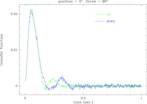
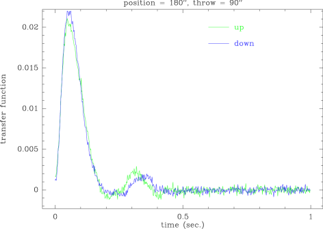
Figure 3: Effects of the non-linearities as seen through transfer functions obtained with rising (“up”) and falling (“down”) step functions (90 arcseconds in amplitude) at two different rest positions (0 and 180 arcseconds for the top and bottom graphs, respectively).

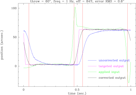
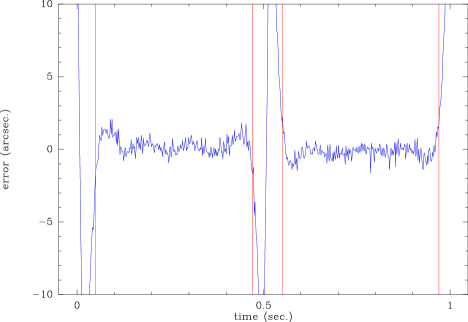
Figure 4: Results obtained with our deconvolution technique for a throw of 60 arcseconds at a frequency of 1 Hz (top). The residual error signal is plotted in the bottom graph and its RMS value (0.6 arcsecond) was calculated using data points located between the vertical lines (on the flatter parts of the curve which represent about 84% of a period).

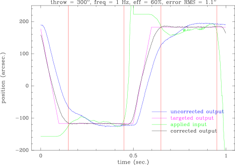
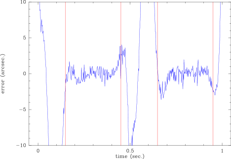
Figure 5: Results obtained with our deconvolution technique for a throw of 300 arcseconds at a frequency of 1 Hz (top). The residual error signal is plotted in the bottom graph and its RMS value (1.1 arcsecond) was calculated using data points located between the vertical lines (on the flatter parts of the curve which represent about 60% of a period).

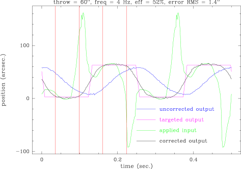
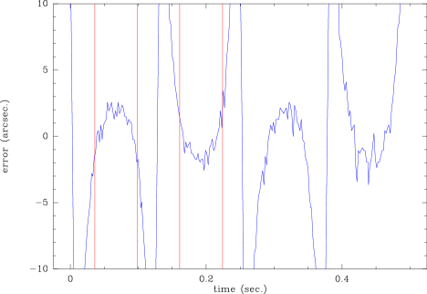
Figure 6: Results obtained with our deconvolution technique for a throw of 60 arcseconds at a frequency of 4 Hz (top). The residual error signal is plotted in the bottom graph and its RMS value (1.4 arcseconds) was calculated using data points located between the vertical lines (on the flatter parts of the curve which represent about 52% of a period).

Figure Captions

Figure 1: The existing chopping secondary mirror assembly at the CSO. A square wave signal is sent to the input of the PID controller and compared with the mirror output position signal (from a LVDT). The resulting processed error signal is sent to a power amplifier which feeds the positioning motor.

Figure 2: The new chopping secondary controller. The new mirror assembly is the same as that of Figure 1, but the input signal is now fed to the PID controller from a RT Linux computer, which hosts the deconvolution program that determines the needed input signal.

Figure 3: Effects of the non-linearities as seen through transfer functions obtained with rising (“up”) and falling (“down”) step functions (90 arcseconds in amplitude) at two different rest positions (0 and 180 arcseconds for the top and bottom graphs, respectively).

Figure 4: Results obtained with our deconvolution technique for a throw of 60 arcseconds at a frequency of 1 Hz (top). The residual error signal is plotted in the bottom graph and its RMS value (0.6 arcsecond) was calculated using data points located between the vertical lines (on the flatter parts of the curve which represent about 84% of a period).

Figure 5: Results obtained with our deconvolution technique for a throw of 300 arcseconds at a frequency of 1 Hz (top). The residual error signal is plotted in the bottom graph and its RMS value (1.1 arcsecond) was calculated using data points located between the vertical lines (on the flatter parts of the curve which represent about 60% of a period).

Figure 6: Results obtained with our deconvolution technique for a throw of 60 arcseconds at a frequency of 4 Hz (top). The residual error signal is plotted in the bottom graph and its RMS value (1.4 arcseconds) was calculated using data points located between the vertical lines (on the flatter parts of the curve which represent about 52% of a period).