The black hole mass versus velocity dispersion relation in QSOs/Active Galactic Nuclei: observational appearance and black hole growth

Abstract

Studies of massive black holes (BHs) in nearby galactic centers have revealed a tight correlation between BH mass and galactic velocity dispersion. In this paper we investigate how the BH mass versus velocity dispersion relation and the nuclear luminosity versus velocity dispersion relation in QSOs/active galactic nuclei (AGNs) are connected with the BH mass versus velocity dispersion relation in local galaxies, through the nuclear luminosity evolution of individual QSOs/AGNs and the mass growth of individual BHs. In the study we ignore the effects of BH mergers and assume that the velocity dispersion does not change significantly during and after the nuclear activity phase. Using the observed correlation in local galaxies and an assumed form of the QSO/AGN luminosity evolution and BH growth, we obtain the simulated observational appearance of the BH mass versus velocity dispersion relation in QSOs/AGNs. The simulation results illustrate how the BH accretion history (e.g., the lifetime of nuclear activity and the possibility that QSOs/AGNs accrete at a super-Eddington accretion rate at the early evolutionary stage) can be inferred from the difference between the relation in QSOs/AGNs and that in local galaxies. We also show how the difference may be weakened by the flux limit of telescopes. We expect that a large complete sample of QSOs/AGNs with accurate BH mass and velocity dispersion measurements will help to quantitatively constrain QSO/AGN luminosity evolution and BH growth models.

1 Introduction

The existence of massive black holes (BHs) in nearby galactic centers, as a prediction of the widely accepted QSO model that QSOs are powered by gas accretion onto massive BHs (e.g., Lynden-Bell 1969; Sołtan 1982; Rees 1984), is now believed to be confirmed (e.g., Kormendy & Richstone, 1995; Magorrian et al., 1998; Gebhardt et al., 2003; Pinkney et al., 2003). Studies of the BHs in nearby galaxies have revealed that BH mass in nearby galactic centers is tightly correlated with galactic velocity dispersion (Ferrarese & Merritt, 2000; Gebhardt et al., 2000a; Tremaine et al., 2002) and is also (less tightly) correlated with the luminosity (or mass) of elliptical galaxies or bulges of spiral/S0 galaxies (e.g., Kormendy & Gebhardt 2001). These correlations suggest a close link between the formation and evolution of BHs and their host galaxies. However, why these correlations exist and whether they also exist in distant galaxies have not yet had definite answers.

The purpose of this paper is to investigate the relationship between BH mass and velocity dispersion in QSOs/active galactic nuclei (AGNs). It is important to study this in QSOs/AGNs at least for the following two reasons:

1. Various BH growth models have been proposed to explain the origin of the tight correlation between BH mass and velocity dispersion in nearby galaxies (e.g., Silk & Rees, 1998; Fabian, 1999; Blandford, 1999; Ostriker, 2000; Haehnelt & Kauffmann, 2000; Burkert & Silk, 2001; Adams et al., 2001; Islam et al., 2003; King, 2003), including accretion of either baryonic gas or non-baryonic dark matter onto seed BHs or hierarchical mergers of intermediate-mass BHs (which might be end products of the first generation of stars, or Population III stars) with masses of typically a few hundred $M\sun$ (e.g., Schneider et al., 2002). How can these BH growth models be tested by observations? Among these BH growth processes, currently BH mergers are unlikely to be observed directly although detecting gravitational wave signals emitted from BH mergers might be possible in the future. The possible observational features of accretion of non-baryonic material are still unclear; only accretion of baryonic gas, which appears as QSO/AGN phenomena, is detectable and has been extensively studied. We expect that the investigation of the BH mass versus velocity dispersion relation in QSOs/AGNs will provide an observationally achievable way to understand BH growth and the origin of the correlation of local BHs with their host galaxies. As a matter of fact, some observational investigations on the relation in QSOs/AGNs have been performed in the past several years (e.g., Laor, 1998; Wandel, 1999; Gebhardt et al., 2000b; Ferrarese et al., 2001; Shields et al., 2003).

2. Furthermore, according to current observations, the total local BH mass density is consistent with the total mass density accreted onto BHs during QSO/AGN phases, which suggests that BH mass growth comes mainly from gas accretion during QSO/AGN phases, rather than from accretion of non-baryonic material or mergers of intermediate-mass BHs (Yu & Tremaine, 2002; Aller & Richstone, 2002; Fabian, 2004). Since QSOs/AGNs represent the population of galaxies housing growing BHs, the study of the relationship between BH mass and velocity dispersion in QSOs/AGNs can provide valuable information on the BH growth history, the evolution of galaxies, and the origin of the tight correlation between BH mass and velocity dispersion in local galaxies.

In this paper we show how the BH mass (or nuclear luminosity) versus velocity dispersion relation in QSOs/AGNs is connected with the BH mass versus velocity dispersion relation in local galaxies through the nuclear luminosity evolution of individual QSOs/AGNs and mass growth of individual BHs. The basic model assumptions are as follows:

1. BH mergers are assumed to not be important for BH growth. In principle, the mass growth of a BH may come from both gas accretion due to QSO/AGN phases and mergers with other BHs. However, currently, the BH merger process and rate are very uncertain. In addition, comparison of the mass density distribution in nearby galaxies with that accreted due to QSO phases has shown that BH mergers are not necessarily required at least for growth of high-mass ($\gtrsim 10^{8}{\rm\,M_{\odot}}$) BHs (Yu & Tremaine, 2002).

2. The velocity dispersion of host galaxies is assumed to not change significantly during and after the nuclear activity phase. In principle, both nuclear luminosity evolution/BH mass growth and the evolution of host galaxy velocity dispersions contribute to the evolution of the nuclear luminosity/BH mass versus velocity dispersion relation. However, ignoring the velocity dispersion evolution may greatly simplify our analysis and highlight the effects of nuclear luminosity evolution/BH mass growth. Comparison of observations with the predictions obtained by ignoring velocity dispersion evolution might also provide clues on the effect of velocity dispersion evolution. In addition, this assumption has also been adopted in many other physical models to explain the correlation between BH mass and velocity dispersion in nearby galaxies (e.g., Silk & Rees 1998; Fabian 1999; Blandford 1999; Burkert & Silk 2001; Adams et al. 2001; King 2003).

The model includes the following three basic components: the BH mass distribution of local galaxies at a given host galaxy velocity dispersion, the curve of the nuclear luminosity evolution/mass growth of individual BHs, and the nuclear luminosity/BH mass distribution in QSOs/AGNs at the given velocity dispersion. In principle, given any two of them, the last one can be constrained by the model. In this paper we use the first two components as model inputs and the third one as the model output.

The paper is organized as follows: In § 2 we review current observational results on the BH mass versus velocity dispersion relation in local galaxies. In § 3 we formulate the connection of the nuclear luminosity/BH mass versus velocity dispersion relation in QSOs/AGNs with the BH mass versus velocity dispersion relation in nearby galaxies through the nuclear luminosity evolution/mass growth of individual BHs. Detailed models on the nuclear luminosity evolution/mass growth of individual BHs are presented in § 4. Applying the observational results of the local BH demography (in § 2) and the assumed QSO luminosity evolution and BH growth curves (in § 4) to the analysis made in § 3, we predict the BH mass versus galactic velocity dispersion relation in QSOs/AGNs and show the simulation results of its observational appearance in § 5. Discussion on current observational results of the relation in QSOs/AGNs is given in § 6. Finally, conclusions are summarized in § 7.

In § 3 readers who are primarily interested in the results of the formulation might want to skip the detailed mathematical manipulations and move straight to the model predictions given by equations (11), (24), and (26) (with the aid of Table 1). The QSO luminosity evolution or BH growth is incorporated into those equations through the lifetime of the nuclear activity $\tau_{\rm life}$ and a distribution function of the probability that the progenitor of a local BH with mass $M_{\rm BH,0}$ (where the subscript “0” represents the current cosmic time $t_{0}$) had a mass $M_{\rm BH}$ or nuclear luminosity $L$ in its nuclear activity history [i.e., $P(M_{\rm BH}|M_{\rm BH,0})$ or $P(L|M_{\rm BH,0})$ in Table 1]. The observational counterparts of the model predictions are given by equations (16) and (30). Comparison of the observations with the model predictions may help to strengthen the existing constraints or provide new information on the QSO/AGN luminosity evolution and BH growth.

In this paper we set the Hubble constant to $H_{0}=100h{\rm\,km\,s^{-1}}$, and the cosmological model used is ($\Omega_{\rm M}$,$\Omega_{\Lambda}$,$h$)$=(0.3,0.7,0.65)$.

2 The BH mass versus velocity dispersion relation in nearby normal galaxies

In nearby galaxies BH mass ($M_{{\rm BH},0}$) is tightly correlated with galactic velocity dispersion ($\sigma$) (Ferrarese & Merritt, 2000; Gebhardt et al., 2000a; Tremaine et al., 2002). The logarithm of the BH mass at a given velocity dispersion $\sigma$ has a mean value given by

$$\langle\log(M_{{\rm BH},0})|\sigma\rangle=A+\gamma\log(\sigma/200{\rm\,km\,s^{-1}})$$ (1)

(Tremaine et al., 2002), where $M_{{\rm BH},0}$ is in units of ${\rm\,M_{\odot}}$, $\gamma=4.02\pm 0.32$, $A=8.18\pm 0.06$ has been adjusted to our assumed Hubble constant $h=0.65$ (see section 2.2 in Yu & Tremaine 2002), and $\sigma$ is the luminosity-weighted line-of-sight velocity dispersion within the effective radius of galaxies. Note that relation (1) is fitted in $\log M_{{\rm BH},0}$–$\log\sigma$ space. We assume that the distribution in $\log M_{{\rm BH},0}$ at a given $\sigma$ is Gaussian, with intrinsic standard deviation ${\Delta_{\log M_{{\rm BH},0}}}$ (which is assumed to be independent of $\sigma$ here), and can be written as

$${\sf p}(\log M_{{\rm BH},0}|\sigma,t_{0})=\frac{1}{\sqrt{2\pi}{\Delta_{\log M_{{\rm BH},0}}}}\exp\left[-\frac{(\log M_{{\rm BH},0}-\langle\log M_{{\rm BH},0}|\sigma\rangle)^{2}}{2\Delta^{2}_{\log M_{{\rm BH},0}}}\right].$$ (2)

According to Tremaine et al. (2002), the intrinsic scatter in $\log M_{{\rm BH},0}$ should not be larger than 0.25–$0.3$  dex. In this paper we set ${\Delta_{\log M_{{\rm BH},0}}}=0.27{\rm\,dex}$.

According to Bayes’s theorem, the velocity dispersion probability distribution function (PDF) of nearby galaxies with BH mass $M_{{\rm BH},0}$, ${\sf p}(\sigma|M_{{\rm BH},0},t_{0})$, is related to
${\sf p}(M_{{\rm BH},0}|\sigma,t_{0})=[\ln(10)M_{{\rm BH},0}]^{-1}{\sf p}(\log M_{{\rm BH},0}|\sigma,t_{0})$ by the equation

$${\sf p}(\sigma|M_{{\rm BH},0},t_{0})=\frac{n_{\sigma}(\sigma,t_{0}){\sf p}(M_{{\rm BH},0}|\sigma,t_{0})}{n_{M_{\rm BH}}(M_{{\rm BH},0},t_{0})},$$ (3)

where $n_{M_{\rm BH}}(M_{{\rm BH},0},t_{0})$ is the local BH mass function (BHMF) defined so that $n_{M_{\rm BH}}(M_{{\rm BH},0},t_{0}){\rm d}M_{{\rm BH},0}$ represents the number density of local BHs with mass in the range $M_{{\rm BH},0}\rightarrow M_{{\rm BH},0}+{\rm d}M_{{\rm BH},0}$, $n_{\sigma}(\sigma,t_{0})$ is the velocity dispersion distribution function of local galaxies with massive BHs, and we have $n_{M_{\rm BH}}(M_{{\rm BH},0},t_{0})=\int n_{\sigma}(\sigma,t_{0}){\sf p}(M_{{\rm BH},0}|\sigma,t_{0}){\rm d}\sigma$.

Besides ${\sf p}(M_{{\rm BH},0}|\sigma,t_{0})$ above, several other PDFs are also defined below. For comparison of their physical meanings, we list all of them in Table 1.

symbol	physical meaning	reference
${\sf p}(M_{{\rm BH},0}|\sigma,t_{0})$	PDF of BH mass in local galaxies with velocity dispersion $\sigma$	eq. 2
${\sf p}(\sigma|M_{{\rm BH},0},t_{0})$	PDF of velocity dispersion in local galaxies with central BH mass $M_{{\rm BH},0}$	eq. 3
$p(L|\sigma,t)$	PDF of nuclear luminosity in QSOs/AGNs with velocity dispersion $\sigma$ at cosmic time $t$	eqs. 4, 15
$p(M_{\rm BH}|\sigma,t)$	PDF of BH mass in QSOs/AGNs with velocity dispersion $\sigma$ at cosmic time $t$	eqs. 22, 29
${\cal P}(L|\sigma)$	PDF of nuclear luminosity in QSOs/AGNs at all redshifts and with velocity dispersion $\sigma$	eqs. 5, 16
${\cal P}(\sigma|L)$	PDF of velocity dispersion in QSOs/AGNs at all redshifts and with nuclear luminosity $L$	eqs. 17, 19
${\cal P}(M_{\rm BH}|\sigma)$	PDF of BH mass in QSOs/AGNs at all redshifts and with velocity dispersion $\sigma$	eqs. 23, 30
$P(L|M_{{\rm BH},0})$	PDF of nuclear luminosity of the progenitor of a local BH during its nuclear activity phases	eq. 8
$P(M_{\rm BH}|M_{{\rm BH},0})$	PDF of BH mass of the progenitor of a local BH during its nuclear activity phases	eq. 25

Table 1: List of PDFs defined in this paper.

3 The demography of QSOs/AGNs

In this section we analytically link the nuclear luminosity/BH mass versus velocity dispersion relation in QSOs/AGNs to the QSO/AGN luminosity evolution, BH growth, and demography of local BHs. We investigate the nuclear luminosity versus velocity dispersion relation in QSOs/AGNs in § 3.1 and the BH mass versus velocity dispersion relation in QSOs/AGNs in § 3.2. For each relation, we first present the model prediction and then show its observational counterpart.

3.1 The nuclear luminosity versus velocity dispersion relation in QSOs/AGNs

3.1.1 Model prediction from local BHs and their nuclear luminosity evolution

We define ${\cal N}_{L}(t_{i},M_{{\rm BH},0},L,t)$ ($t\geq t_{i}$) so that ${\cal N}_{L}(t_{i},M_{{\rm BH},0},L,t){\rm d}t_{i}{\rm d}M_{{\rm BH},0}{\rm d}L{\rm d}t$ is the comoving number density of local BHs with the following properties: the nuclear activity due to accretion onto their seed BHs was triggered during cosmic time $t_{i}\rightarrow t_{i}+{\rm d}t_{i}$, the nuclei of their host galaxies were active and had luminosity in the range $L\rightarrow L+{\rm d}L$ at cosmic time $t$, and the BHs are quiescent and have mass in the range $M_{{\rm BH},0}\rightarrow M_{{\rm BH},0}+{\rm d}M_{{\rm BH},0}$ at the present time $t_{0}$. Thus, the comoving number density of those BHs whose host galaxies have velocity dispersions in the range $\sigma\rightarrow\sigma+{\rm d}\sigma$ is ${\cal N}_{L}(t_{i},M_{{\rm BH},0},L,t){\sf p}(\sigma|M_{{\rm BH},0},t_{0}){\rm d}t_{i}{\rm d}M_{{\rm BH},0}{\rm d}L{\rm d}t{\rm d}\sigma$ [see ${\sf p}(\sigma|M_{{\rm BH},0},t_{0})$ in eq. 3]. We define the PDF of the nuclear luminosity of these BHs at cosmic time $t$ whose host galaxies have velocity dispersion $\sigma$ as follows:

$$p(L|\sigma,t)\equiv\frac{\int_{0}^{t}{\rm d}t_{i}\int{\rm d}M_{{\rm BH},0}~{}{\cal N}_{L}(t_{i},M_{{\rm BH},0},L,t){\sf p}(\sigma|M_{{\rm BH},0},t_{0})}{\int{\rm d}L\int_{0}^{t}{\rm d}t_{i}\int{\rm d}M_{{\rm BH},0}~{}{\cal N}_{L}(t_{i},M_{{\rm BH},0},L,t){\sf p}(\sigma|M_{{\rm BH},0},t_{0})}.$$ (4)

The function ${\cal N}_{L}(t_{i},M_{{\rm BH},0},L,t)$ is controlled by both the rate of triggering accretion onto seed BHs and the luminosity evolution of individual triggered nuclei. The rate of triggering nuclear activity is usually believed to be related to the formation and evolution of galaxies and is a function of cosmic time, which is very uncertain and not easy to predict. The luminosity evolution of individual triggered nuclei is believed to contain information on the accretion process in the vicinity of BHs and is a function of the physical time that the nuclei have spent since the triggering of the accretion onto seed BHs. Note that the luminosity evolution discussed here is different from the evolution of the characteristic luminosity of the QSO population as a function of redshift, which increases with increasing redshift at $z\lesssim 2-3$ and the variation tendency at $z\gtrsim 2-3$ is not yet clear (e.g., see Fig. 6 in Boyle et al. 2000). The luminosity evolution is also not the evolution of the comoving number density of the QSO population as a function of redshift: the comoving number density of QSOs brighter than a certain luminosity has a peak at redshift $z\sim 2-3$ and decreases at both higher and lower redshift. As with ${\cal N}_{L}(t_{i},M_{{\rm BH},0},L,t)$, the PDF $p(L|\sigma,t)$ is partly related to the triggering history and is not easy to predict. By integrating both the numerator and the denominator in equation (4) over the cosmic time $t$, we define a new nuclear luminosity PDF of the BHs with host galactic velocity dispersion $\sigma$ as

$${\cal P}(L|\sigma)\equiv\frac{\int_{0}^{t_{0}}{\rm d}t\int_{0}^{t}{\rm d}t_{i}\int{\rm d}M_{{\rm BH},0}~{}{\cal N}_{L}(t_{i},M_{{\rm BH},0},L,t){\sf p}(\sigma|M_{{\rm BH},0},t_{0})}{\int{\rm d}L\int_{0}^{t_{0}}{\rm d}t\int_{0}^{t}{\rm d}t_{i}\int{\rm d}M_{{\rm BH},0}~{}{\cal N}_{L}(t_{i},M_{{\rm BH},0},L,t){\sf p}(\sigma|M_{{\rm BH},0},t_{0})}.$$ (5)

As is shown below, to obtain the PDF ${\cal P}(L|\sigma)$, the necessary model inputs are only the luminosity evolution of individual triggered nuclei and the local $M_{{\rm BH},0}$-$\sigma$ relation [see also ${\cal P}(M_{\rm BH}|\sigma)$ similarly defined in eq. 23 below].

As done in Yu & Lu (2004), for BHs with the same mass $M_{{\rm BH},0}$ at present, we assume that their nuclear luminosity, ${\cal L}(M_{{\rm BH},0},\tau)$ is a function only of the age of their nuclear activity $\tau\equiv t-t_{i}$. Then we use ${\cal L}(M_{{\rm BH},0},\tau)$ to define two functions to describe the luminosity evolution of individual triggered nuclei. One is the lifetime of the nuclear activity for a BH with mass $M_{{\rm BH},0}$ at present, defined by

$$\tau_{\rm life}(M_{{\rm BH},0}) = \int{\rm d}\tau$$ (6)

$$= \int{\rm d}L\sum_{k}\frac{1}{\left|{\rm d}{\cal L}(M_{{\rm BH},0},\tau)/{\rm d}\tau|_{\tau=\tau_{k}}\right|}$$ (7)

(see eqs. 13 and 14 in Yu & Lu 2004), where the integration in equation (6) is over the period that the nucleus was active and $\tau_{k}(L,M_{{\rm BH},0})$ ($k=1,2,...$) in equation (7) are the roots of the equation ${\cal L}(M_{{\rm BH},0},\tau)-L=0$ ($0<\tau<t_{0}-t_{i}$). Given $L$ and $M_{{\rm BH},0}$, the number of the roots $\tau_{k}$ can be more than 1, since ${\cal L}(M_{{\rm BH},0},\tau)$ can be a non-monotonic function of $\tau$. The other function is a PDF of the nuclear luminosity, defined by

$$P(L|M_{{\rm BH},0})\equiv\frac{1}{\tau_{\rm life}(M_{{\rm BH},0})}\sum_{k}\frac{1}{\left|{\rm d}{\cal L}(M_{{\rm BH},0},\tau)/{\rm d}\tau|_{\tau=\tau_{k}}\right|}$$ (8)

so that $\tau_{\rm life}(M_{{\rm BH},0})P(L|M_{{\rm BH},0}){\rm d}L$ is the time that a BH (with mass $M_{{\rm BH},0}$ at present) spent with nuclear luminosity in the range $L\rightarrow L+{\rm d}L$. According to equation (17) in Yu & Lu (2004), ${\cal N}_{L}(t_{i},M_{{\rm BH},0},L,t)$ is connected with the two functions defined above as follows:

$$\int_{0}^{t_{0}}{\rm d}t\int_{0}^{t}{\rm d}t_{i}~{}{\cal N}_{L}(t_{i},M_{{\rm BH},0},L,t)=\tau_{\rm life}(M_{{\rm BH},0})P(L|M_{{\rm BH},0})n_{M_{\rm BH}}(M_{{\rm BH},0},t_{0}).$$ (9)

Substituting equation (9) into equation (5), we have

$${\cal P}(L|\sigma) = \frac{\int{\rm d}M_{{\rm BH},0}~{}\tau_{\rm life}(M_{{\rm BH},0})P(L|M_{{\rm BH},0})n_{M_{\rm BH}}(M_{{\rm BH},0},t_{0}){\sf p}(\sigma|M_{{\rm BH},0},t_{0})}{\int{\rm d}M_{{\rm BH},0}~{}\tau_{\rm life}(M_{{\rm BH},0})n_{M_{\rm BH}}(M_{{\rm BH},0},t_{0}){\sf p}(\sigma|M_{{\rm BH},0},t_{0})}$$ (10)

$$= \frac{\int{\rm d}M_{{\rm BH},0}~{}\tau_{\rm life}(M_{{\rm BH},0})P(L|M_{{\rm BH},0}){\sf p}(M_{{\rm BH},0}|\sigma,t_{0})}{\int{\rm d}M_{{\rm BH},0}~{}\tau_{\rm life}(M_{{\rm BH},0}){\sf p}(M_{{\rm BH},0}|\sigma,t_{0})},$$ (11)

where equation (3) is used.

3.1.2 Observational counterparts

The PDFs of $p(L|\sigma,t)$ and ${\cal P}(L|\sigma)$ can also be obtained directly from observations of QSOs/AGNs. Assuming that all the local massive BHs have experienced QSO/AGN phases, the observed QSOs/AGNs at redshift $z$ may represent the progenitors of local galaxies and their central BHs at the cosmic time $t(z)$, and the QSO luminosity function (QSOLF) $\Psi_{L}(L,t)$ [defined so that $\Psi_{L}(L,t){\rm d}L$ is the comoving number density of QSOs/AGNs with luminosity in the range $L\rightarrow L+{\rm d}L$ at cosmic time $t$] is given by (see also Yu & Lu 2004)

$$\Psi_{L}(L,t)=\int_{0}^{t}{\rm d}t_{i}\int{\rm d}M_{{\rm BH},0}~{}{\cal N}_{L}(t_{i},M_{{\rm BH},0},L,t).$$ (12)

We can also define the QSO/AGN luminosity and velocity dispersion function (QSOLVF) $\Phi_{LV}(L,\sigma,t)$ so that $\Phi_{LV}(L,\sigma,t){\rm d}L{\rm d}\sigma$ is the comoving number density of QSOs/AGNs with luminosity in the range $L\rightarrow L+{\rm d}L$ at cosmic time $t$ and galactic velocity dispersion in the range $\sigma\rightarrow\sigma+{\rm d}\sigma$; and we have

$$\Psi_{LV}(L,\sigma,t)=\int_{0}^{t}{\rm d}t_{i}\int{\rm d}M_{{\rm BH},0}~{}{\cal N}_{L}(t_{i},M_{{\rm BH},0},L,t){\sf p}(\sigma|M_{{\rm BH},0},t_{0})$$ (13)

$$\Psi_{L}(L,t)=\int\Phi_{LV}(L,\sigma,t){\rm d}\sigma.$$ (14)

Substituting equation (13) into equations (4) and (5), we have

$$p(L|\sigma,t)=\frac{\Phi_{LV}(L,\sigma,t)}{\int{\rm d}L~{}\Phi_{LV}(L,\sigma,t)}$$ (15)

$${\cal P}(L|\sigma)=\frac{\int_{0}^{t_{0}}{\rm d}t~{}\Phi_{LV}(L,\sigma,t)}{\int{\rm d}L\int_{0}^{t_{0}}{\rm d}t~{}\Phi_{LV}(L,\sigma,t)}.$$ (16)

3.1.3 ${\cal P}(\sigma|L)$

Similar to the definition of ${\cal P}(L|\sigma)$, we may also define a velocity dispersion PDF in QSOs/AGNs at a given nuclear luminosity $L$ as follows:

$${\cal P}(\sigma|L) \equiv \frac{\int_{0}^{t_{0}}{\rm d}t\int_{0}^{t}{\rm d}t_{i}\int{\rm d}M_{{\rm BH},0}~{}{\cal N}_{L}(t_{i},M_{{\rm BH},0},L,t){\sf p}(\sigma|M_{{\rm BH},0},t_{0})}{\int{\rm d}\sigma\int_{0}^{t_{0}}{\rm d}t\int_{0}^{t}{\rm d}t_{i}\int{\rm d}M_{{\rm BH},0}~{}{\cal N}_{L}(t_{i},M_{{\rm BH},0},L,t){\sf p}(\sigma|M_{{\rm BH},0},t_{0})}$$ (17)

$$= \frac{\int{\rm d}M_{{\rm BH},0}~{}\tau_{\rm life}(M_{{\rm BH},0})P(L|M_{{\rm BH},0})n_{M_{\rm BH}}(M_{{\rm BH},0},t_{0}){\sf p}(\sigma|M_{{\rm BH},0},t_{0})}{\int{\rm d}M_{{\rm BH},0}~{}\tau_{\rm life}(M_{{\rm BH},0})P(L|M_{{\rm BH},0})n_{M_{\rm BH}}(M_{{\rm BH},0},t_{0})}.$$ (18)

Substituting equations (13) and (14) into equation (18), we have the observational counterpart of ${\cal P}(\sigma|L)$ given by

$${\cal P}(\sigma|L)=\frac{\int_{0}^{t_{0}}{\rm d}t~{}\Phi_{LV}(L,\sigma,t)}{\int_{0}^{t_{0}}{\rm d}t~{}\Psi_{L}(L,t)}$$ (19)

(see also eq. 64 in Yu & Lu 2004).

As a summary of § 3.1, equation (16) or (19) gives the nuclear luminosity versus velocity dispersion relation in QSOs/AGNs directly obtained from observations. Equation (11) or (18) shows the model prediction from the local $M_{{\rm BH},0}$-$\sigma$ relation and the luminosity evolution of individual QSOs/AGNs.

3.2 The BH mass versus velocity dispersion relation in QSOs/AGNs

Given the luminosity evolution of an individual QSO/AGN ${\cal L}_{\rm bol}(M_{{\rm BH},0},t)$ (where the subscript “bol” represents the bolometric luminosity) and the mass-to-energy conversion efficiency $\epsilon$, the BH mass in QSOs/AGNs follows the evolution below:

$${\cal M}_{\rm BH}(M_{{\rm BH},0},\tau)=M_{{\rm BH},i}(M_{{\rm BH},0})+\int_{0}^{\tau}{\rm d}\tau\frac{(1-\epsilon){\cal L}_{\rm bol}(M_{{\rm BH},0},\tau)}{\epsilon c^{2}},$$ (20)

or

$${\cal M}_{\rm BH}(M_{{\rm BH},0},\tau)=M_{{\rm BH},0}-\int_{\tau}^{\tau_{\rm life}(M_{{\rm BH},0})}{\rm d}\tau\frac{(1-\epsilon){\cal L}_{\rm bol}(M_{{\rm BH},0},\tau)}{\epsilon c^{2}},$$ (21)

where $\epsilon$ is assumed to be a constant and $M_{{\rm BH},i}$ is the seed BH mass.

As done in § 3.1, we can also define the BH mass PDF by replacing $L$ and ${\cal L}(M_{{\rm BH},0},\tau)$ with $M_{\rm BH}$ and ${\cal M}_{\rm BH}(M_{{\rm BH},0},\tau)$. First we define ${\cal N}_{M_{\rm BH}}(t_{i},M_{{\rm BH},0},M_{\rm BH},t)$ ($t\geq t_{i}$) so that
${\cal N}_{M_{\rm BH}}(t_{i},M_{{\rm BH},0},M_{\rm BH},t){\rm d}t_{i}{\rm d}M_{{\rm BH},0}{\rm d}M_{\rm BH}{\rm d}t$ is the comoving number density of local BHs with the following properties: the nuclear activity due to accretion onto their seed BHs was triggered during cosmic time $t_{i}\rightarrow t_{i}+{\rm d}t_{i}$, the nuclei of their host galaxies were active with central BH mass in the range $M_{\rm BH}\rightarrow M_{\rm BH}+{\rm d}M_{\rm BH}$ at cosmic time $t$, and these BHs have mass in the range $M_{{\rm BH},0}\rightarrow M_{{\rm BH},0}+{\rm d}M_{{\rm BH},0}$ at present time $t_{0}$. Similar to equations (4) and (5), we can then use ${\cal N}_{M_{\rm BH}}(t_{i},M_{{\rm BH},0},M_{\rm BH},t)$ to define the BH mass PDF in the nuclear-active progenitors of local BHs, for example,

$$p(M_{\rm BH}|\sigma,t)\equiv\frac{\int_{0}^{t}{\rm d}t_{i}\int{\rm d}M_{{\rm BH},0}~{}{\cal N}_{M_{\rm BH}}(t_{i},M_{{\rm BH},0},M_{\rm BH},t){\sf p}(\sigma|M_{{\rm BH},0},t_{0})}{\int{\rm d}M_{\rm BH}\int_{0}^{t}{\rm d}t_{i}\int{\rm d}M_{{\rm BH},0}~{}{\cal N}_{M_{\rm BH}}(t_{i},M_{{\rm BH},0},M_{\rm BH},t){\sf p}(\sigma|M_{{\rm BH},0},t_{0})}$$ (22)

$${\cal P}(M_{\rm BH}|\sigma) \equiv \frac{\int_{0}^{t_{0}}{\rm d}t\int_{0}^{t}{\rm d}t_{i}\int{\rm d}M_{{\rm BH},0}~{}{\cal N}_{M_{\rm BH}}(t_{i},M_{{\rm BH},0},M_{\rm BH},t){\sf p}(\sigma|M_{{\rm BH},0},t_{0})}{\int{\rm d}M_{\rm BH}\int_{0}^{t_{0}}{\rm d}t\int_{0}^{t}{\rm d}t_{i}\int{\rm d}M_{{\rm BH},0}~{}{\cal N}_{M_{\rm BH}}(t_{i},M_{{\rm BH},0},M_{\rm BH},t){\sf p}(\sigma|M_{{\rm BH},0},t_{0})}$$ (23)

$$= \frac{\int{\rm d}M_{{\rm BH},0}~{}\tau_{\rm life}(M_{{\rm BH},0})P(M_{\rm BH}|M_{{\rm BH},0}){\sf p}(M_{{\rm BH},0}|\sigma,t_{0})}{\int{\rm d}M_{{\rm BH},0}~{}\tau_{\rm life}(M_{{\rm BH},0}){\sf p}(M_{{\rm BH},0}|\sigma,t_{0})},$$ (24)

where

$$P(M_{\rm BH}|M_{{\rm BH},0}){\rm d}M_{\rm BH}\equiv\frac{{\rm d}M_{\rm BH}}{\tau_{\rm life}(M_{{\rm BH},0})}\frac{1}{\left|{\rm d}{\cal M}_{\rm BH}(M_{\rm BH},\tau)/{\rm d}\tau\right|_{\tau=\tau_{1}}},$$ (25)

and $\tau_{1}$ is the only root of the equation ${\cal M}_{\rm BH}(M_{{\rm BH},0},\tau)-M_{\rm BH}=0$ ($0<\tau<t_{0}-t_{i}$) [note that ${\cal M}_{\rm BH}(M_{{\rm BH},0},\tau)$ in eq. 20 or 21 is a monotonically increasing function of $\tau$]. The BH growth history (or $\tau_{\rm life}$) may vary for different $M_{{\rm BH},0}$. For simplicity, we assume that $\tau_{\rm life}$ is independent of $M_{{\rm BH},0}$ below, and thus equation (24) becomes

$${\cal P}(M_{\rm BH}|\sigma)=\int P(M_{\rm BH}|M_{{\rm BH},0}){\sf p}(M_{{\rm BH},0}|\sigma,t_{0}){\rm d}M_{{\rm BH},0}.$$ (26)

We can use moments to characterize the distribution of ${\cal P}(\log M_{\rm BH}|\sigma)=\ln(10)M_{\rm BH}{\cal P}(M_{\rm BH}|\sigma)$, such as the mean of $\log M_{\rm BH}$ at a given $\sigma$, defined by

$$\langle\log M_{\rm BH}|\sigma\rangle\equiv\int(\log M_{\rm BH}){\cal P}(\log M_{\rm BH}|\sigma){\rm d}\log M_{\rm BH},$$ (27)

and also the standard variance, the skewness, etc. The difference between the distributions or moments of ${\cal P}(\log M_{\rm BH}|\sigma)$ and ${\sf p}(\log M_{{\rm BH},0}|\sigma,t_{0})$ contains information on BH accretion history and/or galaxy evolution. Obviously, by applying equation (26) to equation (27), we have the difference of the means of the distributions ${\cal P}(M_{\rm BH}|\sigma)$ and ${\sf p}(M_{{\rm BH},0}|\sigma,t_{0})$,

$$\delta\langle\log M_{\rm BH}|\sigma\rangle\equiv\langle\log M_{\rm BH}|\sigma\rangle-\langle\log M_{{\rm BH},0}|\sigma\rangle<0$$ (28)

[note that $P(M_{\rm BH}|M_{{\rm BH},0})=0$ if $M_{\rm BH}>M_{{\rm BH},0}$, and see $\langle\log M_{{\rm BH},0}|\sigma\rangle$ in eq. 1]. A positive difference of the means might suggest that galaxy velocity dispersions should increase during or after the nuclear activity (i.e., the assumption that the velocity dispersion does not significantly change during or after the nuclear activity should be revised).

Similar to defining the QSOLVF as $\Phi_{LV}(M_{\rm BH},\sigma,t)$ in § 3.1, we can define the BH mass and velocity dispersion function in QSOs/AGNs (QSOMVF) as $\Phi_{MV}(M_{\rm BH},\sigma,t)$, so that $\Phi_{MV}(M_{\rm BH},\sigma,t){\rm d}M_{\rm BH}{\rm d}\sigma$ represents the comoving number density of QSOs/AGNs with central BH mass in the range $M_{\rm BH}\rightarrow M_{\rm BH}+{\rm d}M_{\rm BH}$ and host galactic velocity dispersion in the range $\sigma+{\rm d}\sigma$ at cosmic time $t$. Thus we have

$$p(M_{\rm BH}|\sigma,t)=\frac{\Phi_{MV}(M_{\rm BH},\sigma,t)}{\int{\rm d}M_{\rm BH}~{}\Phi_{MV}(M_{\rm BH},\sigma,t)}$$ (29)

$${\cal P}(M_{\rm BH}|\sigma)=\frac{\int_{0}^{t_{0}}{\rm d}t~{}\Phi_{MV}(M_{\rm BH},\sigma,t)}{\int{\rm d}M_{\rm BH}\int_{0}^{t_{0}}{\rm d}t~{}\Phi_{MV}(M_{\rm BH},\sigma,t)}.$$ (30)

The distributions of $p(M_{\rm BH}|\sigma,t)$ and ${\cal P}(M_{\rm BH}|\sigma)$ give the BH mass versus velocity dispersion relations for QSOs/AGNs at a given cosmic time and for QSOs/AGNs at all redshifts, respectively. The ${\cal P}(M_{\rm BH}|\sigma)$ is the $M_{\rm BH}$-$\sigma$ relation in QSOs/AGNs that is mainly discussed in this paper.

Comparison of the expectation from equation (26) (or [24], [11], [18]) with observations of QSOs/AGNs (see eq. [30], [16], or [19]) can provide feedback to our understanding of the luminosity evolution of individual QSOs/AGNs, the mass growth of individual BHs, and the evolution of host galaxy velocity dispersions.

4 The QSO/AGN luminosity evolution and BH growth model: ${\cal L}_{\rm bol}(M_{{\rm BH},0},\tau)$ and ${\cal M}_{\rm BH}(M_{{\rm BH},0},\tau)$

In this section we present the detailed form of the luminosity evolution and BH growth [${\cal L}_{\rm bol}(M_{{\rm BH},0},\tau)$ and ${\cal M}_{\rm BH}(M_{{\rm BH},0},\tau)$] incorporated in the analysis in § 3. We assume that the luminosity evolution of individual QSOs/AGNs can be described by two phases (see also § 2.4 in Yu & Lu 2004): (1) after the accretion onto a seed BH is triggered, initially there is sufficient material to feed the BH, and the BH accretes with Eddington luminosity; (2) with the mass growth of the BHs and the consumption of the material to feed it, the material becomes insufficient to support Eddington accretion, and then the nuclear luminosity declines and is fainter than the Eddington luminosity (see also Yu & Lu 2004). For simplicity, below we assume that the two phases appear only once for each BH (see also Yu & Lu 2004).

We assume that the first phase lasts for a period of $\tau_{\rm I}$, and the BH mass increases to $M_{{\rm BH,I}}$ at time $t=t_{i}+\tau_{\rm I}\equiv t_{\rm I}$. Thus, the nuclear luminosity in the first phase increases with time as

$${\cal L}_{\rm bol}(\tau)=L_{\rm Edd}(M_{{\rm BH,I}})\exp\left(\frac{\tau-\tau_{\rm I}}{\tau_{\rm Sp}}\right)\qquad 0<\tau<\tau_{\rm I},$$ (31)

where $L_{\rm Edd}(M_{{\rm BH,I}})$ is the Eddington luminosity of a BH with mass $M_{{\rm BH,I}}$, and

$$\tau_{\rm Sp}=4.5\times 10^{7}\left[\frac{\epsilon}{0.1(1-\epsilon)}\right]{\rm\,yr}$$ (32)

is the Salpeter time (the time required for a BH radiating at Eddington luminosity to $e$-fold in mass). The BH mass increases as

$${\cal M}_{\rm BH}(\tau)=M_{{\rm BH,I}}\exp\left(\frac{\tau-\tau_{\rm I}}{\tau_{\rm Sp}}\right)\qquad 0<\tau<\tau_{\rm I}.$$ (33)

In the second phase we assume that the evolution of the nuclear luminosity declines as

$${\cal L}_{\rm bol}(\tau)=\cases{L_{\rm Edd}(M_{{\rm BH,I}})\exp\left(-\frac{\tau-\tau_{\rm I}}{\tau_{\rm D}}\right),&for $\tau_{\rm I}\leq\tau\leq\tau_{\rm I}+\xi\tau_{\rm D}$,\cr 0,&for $\tau>\tau_{\rm I}+\xi\tau_{\rm D}$,}$$ (34)

where $\tau_{\rm D}$ is the characteristic declining timescale of the nuclear luminosity. We assume that QSOs/AGNs become quiescent when the nuclear luminosity declines by a factor of $\eta=\exp(-\xi)$ compared to the peak luminosity $L_{\rm Edd}(M_{{\rm BH,I}})$, so there is a cutoff of the nuclear luminosity at $\tau=\tau_{\rm I}+\xi\tau_{\rm D}$ in equation (34). The factor $\xi$ is set to $\ln(10^{3})=6.9$ (as in Yu & Lu 2004). According to equations (20) and (34), the BH mass increases as

$${\cal M}_{\rm BH}(\tau)=M_{{\rm BH,I}}\left\{1+\frac{\tau_{\rm D}}{\tau_{\rm Sp}}\left[1-\exp\left(\frac{\tau_{\rm I}-\tau}{\tau_{\rm D}}\right)\right]\right\},\qquad\tau_{\rm I}\leq\tau\leq\tau_{\rm I}+\xi\tau_{\rm D}.$$ (35)

With the assumption that the nuclear activity of all QSOs/AGNs is quenched at present (i.e., $t_{0}-t_{i}-\tau_{\rm I}\gg\tau_{\rm D}$), the BH mass at present is given by

$$M_{{\rm BH},0}=\left(1+\frac{\tau_{\rm D}}{\tau_{\rm Sp}}\right)M_{{\rm BH,I}}.$$ (36)

Some constraints on ${\cal L}_{\rm bol}(M_{{\rm BH},0},\tau)$ have been obtained by comparing the time integral of the QSOLF in observations with the prediction from the local BHMF in Yu & Lu (2004). For example, for the nuclear luminosity evolution models above, we should have $\tau_{\rm I}\gtrsim\tau_{\rm Sp}$ if $\epsilon\sim 0.1$ and $\tau_{\rm D}=0$ and have $\tau_{I}\gtrsim 0.2\tau_{\rm Sp}$ if $\epsilon\sim 0.31$ and $\tau_{\rm D}=0$. The characteristic declining timescale of the second phase, $\tau_{\rm D}$, should be significantly shorter than $\tau_{\rm Sp}$, and BH growth should not be dominated by accretion in the second phase. In this paper, based on those constraints, we assume two family models for the parameter $\tau_{\rm D}$: (1) $\tau_{D}=0$ and (2) $\tau_{D}=0.3\tau_{\rm Sp}$. In each of the family models, we consider four cases for the total mass increase of a BH during its nuclear activity period: that is, $M_{{\rm BH},0}/M_{{\rm BH},i}=\exp(0.3),\exp(1),\exp(2)$, and $\exp(4)$, which are denoted as cases A-D, respectively. Thus, we have $\tau_{\rm D}=0$ and $\tau_{\rm I}/\tau_{\rm Sp}=0.3,~{}1,~{}2$, and $4$ for models 1A-1D; and we have $\tau_{\rm D}/\tau_{\rm Sp}=0.3$ and $\tau_{\rm I}/\tau_{\rm Sp}=0.04,~{}0.7,~{}1.7$, and $3.7$ for models 2A-2D.

5 Simulation results of the $M_{\rm BH}$-$\sigma$ relation in QSOs/AGNs

In this section, by applying the BH growth models in § 4 to the analysis in § 3, we obtain the expected observational appearance of the $M_{\rm BH}$-$\sigma$ relation in QSOs/AGNs. We quantitatively illustrate how this relation in QSOs/AGNs depends on the BH growth history and how the flux limit of telescopes affects the observational appearance of the relation. Similarly, the expected observational appearance of the $L$-$\sigma$ relation in QSOs/AGNs can also be obtained, but for simplicity we do not show and discuss it in this paper.

5.1 $\tau_{\rm I}$ and $\tau_{\rm D}$

With the local $M_{{\rm BH},0}$-$\sigma$ relation [or ${\sf p}(M_{{\rm BH},0}|\sigma,t_{0})$; see eqs. 1 and 2] and the QSO/AGN luminosity evolution and BH growth models described in § 4, we use equation (26) to get the distribution ${\cal P}(M_{\rm BH}|\sigma)$ in QSOs/AGNs. The results of ${\cal P}(\log M_{\rm BH}|\sigma=200{\rm\,km\,s^{-1}})$ are shown in Figure 1a for model 1 and in Figure 1b for model 2. In each panel we show the distribution in nearby normal galaxies, ${\sf p}(\log M_{{\rm BH},0}|\sigma,t_{0})$, by the solid line and show the distribution in QSOs/AGNs, ${\cal P}(\log M_{\rm BH}|\sigma)$, by the dotted, short-dashed, dot-dashed, and long-dashed lines for cases A-D, respectively. Note that the shape of the distribution ${\sf p}(\log M_{{\rm BH},0}|\sigma,t_{0})$ has been assumed to be independent of $\sigma$, and the characteristic increasing and decreasing timescales ($\tau_{\rm I}$, $\tau_{\rm D}$) have been assumed to be independent of $M_{{\rm BH},0}$; therefore, the shapes of the curves of ${\cal P}(\log M_{\rm BH}|\sigma)$ are independent of $\sigma$, and the distributions for other velocity dispersions can be obtained simply by shifting the curves to higher or lower BH masses. The difference of the distributions ${\cal P}(\log M_{\rm BH}|\sigma)$ and ${\sf p}(\log M_{{\rm BH},0}|\sigma,t_{0})$ can be characterized by the difference of the mean ($\delta\langle\log M_{\rm BH}|\sigma\rangle$ in eq. 28), the standard variance, the skewness, etc. For simplicity, we mainly discuss the difference of the mean below.

As seen from Figure 1, with increasing timescale $\tau_{\rm I}$ (see eq. 31), the curve peak of ${\cal P}(\log M_{\rm BH}|\sigma)$ shifts to low BH mass and the scatter of ${\cal P}(\log M_{\rm BH}|\sigma)$ increases, since the probability of observing QSOs/AGNs with low BH masses increases. Our calculations show that we have the difference $\delta\langle\log M_{\rm BH}\rangle=\log(M_{{\rm BH},i}/M_{{\rm BH},0})/2\simeq-0.07,-0.2,-0.4$ and $,-0.9$  dexfor models 1A-1D in panel (a) and $\delta\langle\log M_{\rm BH}\rangle\simeq-0.02,-0.08,-0.2$, and $-0.6$  dexfor models 2A-2D in Figure 1b. The difference $\delta\langle\log M_{\rm BH}\rangle$ is difficult to detect for cases (A) and (B), considering the current large measurement errors of BH masses in QSOs/AGNs (see the discussion in § 6), and the difference is relatively significant for case D, which should be detectable if there existed a sufficiently large and complete sample of QSOs/AGNs. As seen from Figure 1, for the same case of the two family models, compared to model 1 ($\tau_{\rm D}=0$), ${\cal P}(\log M_{\rm BH}|\sigma)$ in model 2 ($\tau_{\rm D}=0.3\tau_{\rm Sp}$) is lower at the low-mass end and higher at the high-mass end, and the peak of the curve is closer to the peak of the local distribution ${\sf p}(\log M_{{\rm BH},0}|\sigma,t_{0})$, although the BH mass is increased by the same factor during the nuclear activity. The reason is that in model 2, QSOs/AGNs have a substantially large probability of being observed in the second phase (see eq. 34), in which the QSOs/AGNs are shining at sub-Eddington luminosities and BH masses grow relatively slowly and have acquired nearly all of their mass. In addition, Figure 1(b) shows that the existence of sub-Eddington accretion at the late evolutionary stage may also introduce skewness to the distribution of ${\cal P}(\log M_{\rm BH}|\sigma)$.

5.2 Super-Eddington accretion

In Figure 1 the nuclear luminosity has been assumed to be limited by the Eddington luminosity. In the literature, however, it is argued that QSOs/AGNs might be able to accrete material at a rate higher than the Eddington accretion rate (which is conventionally defined by the Eddington luminosity for $\epsilon=0.1$ here) at the early stage of their evolution (since initially the material supply for the BH growth may be sufficiently large; e.g., Blandford 2004). Below we use a simple example to illustrate how the $M_{\rm BH}$-$\sigma$ relation in QSOs/AGNs is affected by super-Eddington accretion.

We modify model 1D ($\tau_{\rm I}/\tau_{\rm Sp}=4$) as follows: BHs first accrete material at a rate higher than the Eddington rate by a factor of $l$ in the initial $3\tau^{\prime}_{\rm Sp}$ period of the nuclear activity, where $l$ is a constant and $\tau^{\prime}_{\rm Sp}=l^{-1}\tau_{\rm Sp}$ (eq. 32), and then BHs accrete material at the Eddington rate for a period of $\tau_{\rm Sp}$. We denote the modified model as model 1D^′. The BH mass is increased by the same factor in the initial $3\tau^{\prime}_{\rm Sp}$ period of the nuclear activity in model 1D^′ as that in the initial $3\tau_{\rm Sp}$ period of the nuclear activity in model 1D. The total BH mass increase over the whole nuclear activity period is also the same in models 1D^′ and 1D. The ${\cal P}(\log M_{\rm BH}|\sigma)$ of model 1D^′ are shown as the dotted ($l=2$) and dot-dashed ($l=10$) lines in Figure 2. For comparison, ${\sf p}(\log M_{{\rm BH},0}|\sigma,t_{0})$ and the results of models 1B ($\tau_{\rm I}/\tau_{\rm Sp}=1$) and 1D shown in Figure 1a are also shown in Figure 2 as the solid, short-dashed, and long-dashed lines, respectively. As seen from Figure 2, the dot-dashed line (model 1D^′ with $l=10$) is lower than both the dotted (model 1D^′ with $l=2$) and long-dashed lines (model 1D) at the low-mass end ($\lesssim 10^{7}{\rm\,M_{\odot}}$), and the distribution of the dot-dashed line is closer to that of the short-dashed line (model 1B; $\tau_{\rm I}/\tau_{\rm Sp}=1$) than that of the dotted line. The reason is that the larger the accretion rate, the more rapidly the BH mass increases, and thus the smaller the probability of the low-mass BHs within a unit mass range being observed, since the high-rate or super-Eddington accretion is at the early BH growth stage here. For example, in model 1D^′, the BH mass increases by a factor of $\sim 20$ at the early super-Eddington accretion stage and by a factor of $\sim 2.7$ at the Eddington accretion stage; for the case of $l=2$, the time fractions for a QSO to be at those stages are 60% and 40%, respectively, but for the case of $l=10$, the corresponding time fractions become only 23% and up to 77%. The effect of the super-Eddington accretion can also be quantitatively characterized by high-order moments of ${\cal P}(\log M_{\rm BH}|\sigma)$, such as skewness.

5.3 Effects of the flux limit of telescopes

In the results above, we have assumed that QSOs/AGNs with any luminosities can be observed, without being limited by the flux limit of telescopes. In this subsection we show how the observational appearance of the $M_{\rm BH}$-$\sigma$ relation in QSOs/AGNs is affected if only those QSOs/AGNs brighter than a certain absolute magnitude are detected. We show the results of ${\cal P}^{\prime}(\log M_{\rm BH}|\sigma)$, the portion of ${\cal P}(\log M_{\rm BH}|\sigma)$ contributed to QSOs/AGNs with such absolute magnitude truncations, in Figure 3. Unlike those of ${\cal P}(\log M_{\rm BH}|\sigma)$ in Figures 1 and 2, the shapes of ${\cal P}^{\prime}(\log M_{\rm BH}|\sigma)$ vary for different galactic velocity dispersions because of the magnitude truncation. Thus, we show the results at two different velocity dispersions: $\sigma=200{\rm\,km\,s^{-1}}$ in Figure 3a and 3b, and $\sigma=320{\rm\,km\,s^{-1}}$ in Figure 3c and 3d. For $\sigma=200{\rm\,km\,s^{-1}}$ we set the magnitude truncation of the QSOs/AGNs to be $M_{B}<-20$ and $-23$ (the bolometric correction for the $B$-band luminosity, $C_{B}$, is defined through $L_{\rm bol}\equiv C_{B}L_{\nu_{B}}$, where $L_{\nu_{B}}$ is the energy radiated at the central frequency of the $B$ band per unit time and logarithmic interval of frequency, and we set $C_{B}=11.8$; see Elvis et al. 1994). For the high-velocity dispersion $\sigma=320{\rm\,km\,s^{-1}}$, we set a brighter magnitude truncation ($M_{B}<-23$ and $-25$) because of the following considerations: at $z\lesssim$ 2–3 the characteristic luminosity of QSOs/AGNs increases with the increase of redshift (see the QSOLF given in Boyle et al. 2000), or high-mass BHs are more likely to grow up at high redshifts, and for high-redshift objects, only the bright ones are observed. Other model parameters in Figure 3 ($\tau_{\rm I}$, $\tau_{\rm D}$) are the same as those in models 2A-2D (see Fig. 1b). As seen from Figure 3, QSOs/AGNs housing small BHs cannot be detected because of the faintness cutoff. The distribution of ${\cal P}^{\prime}(\log M_{\rm BH}|\sigma)$ is also lower than that of ${\cal P}(\log M_{\rm BH}|\sigma)$ at the high-mass end because some QSOs/AGNs that house big BHs but are at the late stage of the second luminosity evolutionary phase (eq. 34) may also be missing from observations. Our calculations show that if the sample of QSOs with $M_{B}<-20$ is complete, $|\delta\langle\log M_{\rm BH}\rangle|$ is about $0.6$  dexat $\sigma=200{\rm\,km\,s^{-1}}$ for model 2D (see the long-dashed line in Fig. 3a), which is detectable if the accuracy of the BH mass measurement is within a factor of $\sim 2$-$3$. However, if the magnitude truncation is $M_{B}<-23$, we have the difference $|\delta\langle\log M_{\rm BH}\rangle|\lesssim 0.1{\rm\,dex}$ at $\sigma=200{\rm\,km\,s^{-1}}$ (see Fig. 3b), which is too small to detect currently. In short, Figure 3 suggests that the flux limit of telescopes may weaken the difference of the observed $M_{\rm BH}$-$\sigma$ relation in QSOs/AGNs from the local $M_{{\rm BH},0}$-$\sigma$ relation, since small BHs, the main contributors to the difference of these relations, may be missing from observations.

To further illustrate the appearance of the $M_{\rm BH}$-$\sigma$ relation in QSOs/AGNs, we simulate a sample of local galaxies and QSOs/AGNs and show the result in an $M_{\rm BH}$ versus $\sigma$ plot (see the black dots for local galaxies and red dots for QSOs/AGNs in Fig. 4). To do this, we first use the Monte-Carlo method to draw a sample of $10^{4}$ galaxies from the velocity dispersion distribution of local galaxies with $\sigma>80{\rm\,km\,s^{-1}}$ (see the black dots in Fig. 4; for the velocity dispersion distribution of local galaxies, see Yu & Lu 2004). Then, for each (local) galaxy, we use the Monte-Carlo method to generate one progenitor (i.e., QSOs/AGNs) from the distribution function ${\cal P}(M_{\rm BH}|\sigma)$. Note that the number of progenitors generated for each local galaxy, which should be proportional to the lifetime of the nuclear activity of this galaxy $\tau_{\rm life}$, is the same, since the lifetime has been assumed to be the same for all the galaxies here. In addition, although only one progenitor is produced for each galaxy, the total number of progenitors generated for all the galaxies is large enough in this paper to illustrate the appearance of the $M_{\rm BH}$-i$\sigma$ relation in QSOs/AGNs. Finally, we cut off faint progenitors, and the rest are just the sample of QSOs/AGNs with magnitude truncation (red dots in Fig. 4). We show the results of models 2C and 2D ($\tau_{\rm D}/\tau_{\rm Sp}=0.3$, $\tau_{\rm I}/\tau_{\rm Sp}=2,4$) with an absolute magnitude truncation of $M_{B}<-20$ in Figures 4a and 4b, and show the results of models 2C and 2D with $M_{B}<-23$ in Figures 4c and 4d, respectively. The simulation results of models 2A and 2B are not shown in this figure because they are visually difficult to distinguish from the local $M_{{\rm BH},0}$-$\sigma$ relation. In models 2C and 2D, the increase of the BH mass via accretion is large enough (e.g., by a factor of $\gtrsim 10$) that as seen from Figures 4a and 4b, if all or at least most of the QSOs/AGNs with absolute magnitude $M_{B}<-20$ can be detected, many red dots with small BH masses (simulated QSOs/AGNs) will be below the black dots (simulated local galaxies), and the $M_{\rm BH}$-$\sigma$ relation in QSOs/AGNs will be easily distinguished from the local $M_{{\rm BH},0}$-$\sigma$ relation. However, the $M_{\rm BH}-\sigma$ relations with truncation $M_{B}<-23$ in Figures 4c and 4d are not as easy to distinguish from the local $M_{{\rm BH},0}$-$\sigma$ relation as those in Figures 4a and 4b, since QSOs/AGNs housing small BHs are missing from observations.

In addition, the observational appearance of the $M_{\rm BH}$-$\sigma$ relation in QSOs/AGNs may also be affected by obscuration. If QSOs/AGNs at the early evolutionary stage are strongly obscured, as suggested by Fabian (1999) and King (2003), the $M_{\rm BH}$-$\sigma$ relation in the observed QSOs/AGNs should be less deviated from the $M_{{\rm BH},0}$-$\sigma$ relation in nearby galaxies, since the early stage of BH growth is missing from observations. However, if the obscuration is a purely geometric effect (as suggested by the unification model of QSOs/AGNs) and the obscured fraction does not depend on the QSO/AGN luminosity or central BH mass, the observational appearance of the $M_{\rm BH}$-$\sigma$ relation will not be affected by obscuration.

Figure 1: Estimated BH mass distribution in QSOs/AGNs [i.e., ${\cal P}(\log M_{\rm BH}|\sigma)$; see eq. 26] at a given host galaxy velocity dispersion $\sigma=200{\rm\,km\,s^{-1}}$. The luminosity evolution and BH growth models used are described in § 4. In (a) are the results for model 1 ($\tau_{\rm D}=0$) and (b) is for model 2 ($\tau_{\rm D}/\tau_{\rm Sp}=0.3$). In both panels, the solid line represents ${\sf p}(\log M_{{\rm BH},0}|\sigma,t_{0})$ (or the local $M_{{\rm BH},0}$-$\sigma$ relation, for which a Gaussian distribution of $\log M_{\rm BH}$ is assumed with an intrinsic scatter of $0.27$  dex; see eqs. 1 and 2). The dotted, short-dashed, dot-dashed, and long-dashed lines represent the results obtained by setting $\ln(M_{{\rm BH},0}/M_{{\rm BH},i})=0.3,1,2$, and $4$ (which are denoted by cases A-D, respectively). That is, we have $\tau_{\rm I}/\tau_{\rm Sp}=0.3,1,2$,and $4$ for models 1A-1D in (a), and have $\tau_{\rm I}/\tau_{\rm Sp}=0.04,0.7,1.7$, and $3.7$ for models 2A-2D in (b). As seen from this figure, with increasing $\tau_{\rm I}$ the probability of ${\cal P}(\log M_{\rm BH}|\sigma)$ at the low-mass end increases, and the deviation of ${\cal P}(\log M_{\rm BH}|\sigma)$ from ${\sf p}(\log M_{{\rm BH},0}|\sigma,t_{0})$ increases. Compared to the results of the purely Eddington accretion model in (a), the existence of sub-Eddington accretion at the late evolution stage ($\tau_{\rm D}\neq 0$ in [b]) decreases the difference $|\delta\langle\log M_{\rm BH}\rangle|$ (eq. 28) and also may introduce skewness to the distribution of ${\cal P}(\log M_{\rm BH}|\sigma)$. See details in § 5.1.

Figure 2: Estimated BH mass distribution ${\cal P}(\log M_{\rm BH}|\sigma)$ in QSOs/AGNs at a given host galaxy velocity dispersion, for which a super-Eddington accretion at the early evolutionary stage of the nuclear activity is assumed. The solid, short-dashed, and long-dashed lines are the same as those in Figure 1(a). The dotted and dot-dashed lines represent the results obtained by model 1D^′, assuming that BHs accrete material at the Eddington rate only at the final $\tau_{\rm Sp}$ period of the nuclear activity. Before that period, BHs accrete at a rate higher than the Eddington rate, for example, by a factor of 2 (dotted line) or 10 (dot-dashed line). As seen from this figure, super-Eddington accretion at the early stage decreases ${\cal P}(M_{\rm BH}|\sigma)$ at the low-mass end and may also introduce skewness to the distribution ${\cal P}(\log M_{\rm BH}|\sigma)$. See details in § 5.2.

Figure 3: Estimated ${\cal P}^{\prime}(\log M_{\rm BH}|\sigma)$, i.e., the portion of ${\cal P}(\log M_{\rm BH}|\sigma)$ contributed to by QSOs/AGNs brighter than a certain absolute magnitude. The line types have the same meanings as in Figure 1. The $B$-band absolute magnitude truncations are $M_{B}<-20,-23$, and $-25$ in (a), (b-c), and (d), respectively. Other model parameters ($\tau_{\rm I}$, $\tau_{\rm D}$) are the same as in model 2 (see Fig. 1b). Panels a and b are for the distributions at $\sigma=200{\rm\,km\,s^{-1}}$, and panels c and d are for the distributions at $\sigma=320{\rm\,km\,s^{-1}}$. This figure (and also Fig. 4 below) suggests that the flux limit of telescopes may decrease the difference $|\delta\langle\log M_{\rm BH}\rangle|$ between the observed $M_{\rm BH}$-$\sigma$ relation in QSOs/AGNs and the $M_{{\rm BH},0}$-$\sigma$ relation in local galaxies, since small BHs, the main contributors to the difference, may be missing from observations. See details in § 5.3.

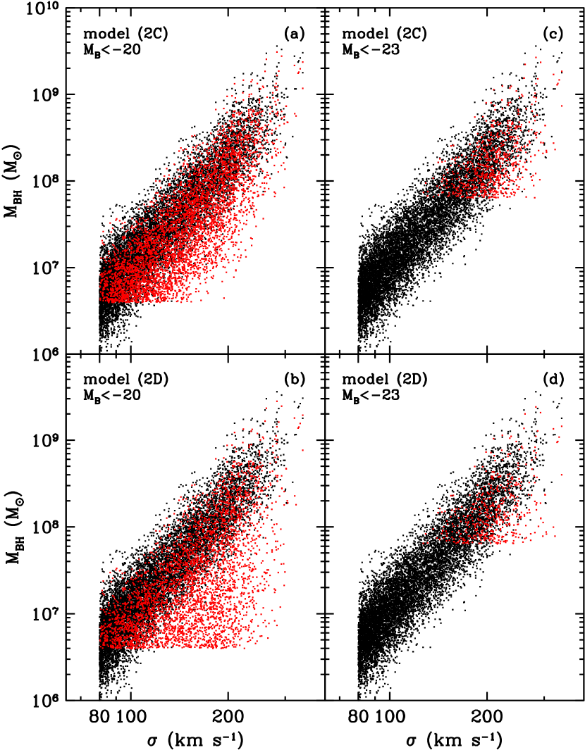
Figure 4: Simulation results of the $M_{\rm BH}$-$\sigma$ relation in QSOs/AGNs. The black dots represent local galaxies with an assumed intrinsic scatter in $\log M_{{\rm BH},0}$ of $0.27$  dex, and the red dots represent QSOs/AGNs. Panels a and c are for model 2C, and panels b and d are for model 2D. Panels a and b only include QSOs/AGNs with $M_{B}<-20$, and panels c and d only include QSOs/AGNs with $M_{B}<-23$. Each panel has $10^{4}$ black dots; and the numbers of red dots are 4276, 3562, 658, and 462 in panels (a-d), respectively. See details in § 5.3.

6 Discussion on current observational results of QSOs/AGNs

Some observations of the BH mass/nuclear luminosity versus velocity dispersion relation in QSOs/AGNs have been made in the past several years (e.g., Laor, 1998; Wandel, 1999; Gebhardt et al., 2000b; Ferrarese et al., 2001; Shields et al., 2003). For example, Gebhardt et al. (2000b) and Ferrarese et al. (2001) argue that QSOs/AGNs follow the same BH mass versus velocity dispersion relation as local galaxies based on some galaxy samples including a small number (seven or six) of QSOs/AGNs that have measurements of both BH masses and velocity dispersions. The masses of BHs in QSOs/AGNs in these studies are estimated by the reverberation mapping technique (e.g., Wandel et al., 1999; Kaspi et al., 2000). However, Krolik (2001) argues that the BH mass measured by this method may be either underestimated or overestimated by a systematic error of up to a factor of $\sim 3$, partly because of the deviation of the simple assumptions on the dynamics/kinematics and the geometry of broad-line regions from the reality. For another example, Shields et al. (2003) use a larger sample of QSOs/AGNs ($\sim 100$, including $\sim 20$ high-redshift [$z\gtrsim 1$] QSOs) with estimated BH mass and velocity dispersion and also argue that the BH mass versus velocity dispersion relation in QSOs/AGNs is consistent with the relation in nearby galaxies. In Shields et al. (2003), the BH mass is estimated through the empirical law between BH mass and broad-line region size (e.g., Kaspi et al., 2000) and the [OIII] line width is used as a surrogate for the galactic velocity dispersion (e.g., Nelson, 2000). These methods might introduce further uncertainties in BH mass and velocity dispersion. Despite the measurement error (or possible systematic error) in BH mass and velocity dispersions, we note that the flux limit of telescopes can still cause consistency between the relations in Shields et al. (2003), especially for the subsample of high-redshift QSOs (which include only BHs with masses higher than $10^{9}{\rm\,M_{\odot}}$). Just as illustrated in Figures 3 and  4, since low-mass progenitors of big BHs are not detected, the relation in QSOs/AGNs is difficult to distinguish from that in local galaxies.

Ignoring possible (systematic) measurement errors in BH masses and velocity dispersions or selection effects for the samples of QSOs/AGNs in Gebhardt et al. (2000b) and Ferrarese et al. (2001), we give a tentative discussion below on the possible implications of their results. The BH masses in QSOs/AGNs have a negative offset of $-0.21{\rm\,dex}$ from local BHs for the sample in Gebhardt et al. (2000b) (including seven QSOs/AGNs) but have a positive offset for the sample in Ferrarese et al. (2001) (including six QSOs/AGNs). According to equation (28), a positive offset might mean that the velocity dispersion increases during or after the nuclear activity. However, here we think that the difference of the offsets for these two different samples is partly because (1) the slope of the local $M_{{\rm BH},0}$-$\sigma$ relation (see $\gamma$ in eq. 1) in Ferrarese et al. (2001) is steeper than that in Gebhardt et al. (2000b), and (2) the velocity dispersions of two AGNs (NGC 4051 and NGC 4151, which are included in both samples) measured in Ferrarese et al. (2001) are smaller than those quoted in Gebhardt et al. (2000b) by $\sim 10\%$. According to Gebhardt et al. (2000b), the offset of the $M_{\rm BH}-\sigma$ relation in QSOs/AGNs from the $M_{{\rm BH},0}-\sigma$ relation in nearby galaxies can be down to $-0.21$dex. The amount of the offset, based on the calculation results illustrated in Figure 1(a) and (b), suggests that the period in which QSOs/AGNs accrete material with Eddington luminosity can be as long as $\sim 1$–$2\tau_{\rm Sp}$ and the BH mass can be increased by a factor of up to $\sim$3–8 [i.e., $\sim\exp(1)$–$\exp(2)$] during the nuclear activity (this suggestion does not contradict the result obtained in Yu & Tremaine 2002 and Aller & Richstone 2002 that local BH mass comes mainly from accretion during QSO phases).

Since current samples of QSOs/AGNs with BH mass and velocity dispersion measurements suffer from the uncertainty of small number statistics, large measurement errors, and incompleteness due to the flux limit of telescopes, a large complete sample of QSOs/AGNs with accurate BH mass and velocity dispersion measurements is needed to obtain quantitative constraints on the BH accretion history from the comparison of the BH mass versus velocity dispersion relation in QSOs/AGNs with that in local galaxies.

7 Conclusions

In this paper we have investigated how the BH mass/nuclear luminosity versus velocity dispersion relation in QSOs/AGNs is connected with the local BH mass versus velocity dispersion relation through the mass growth/nuclear luminosity evolution of individual BHs (see eqs. 24 and 11), by ignoring BH mergers and assuming that the velocity dispersion does not significantly change during and after the nuclear activity phase. Circumventing the uncertain history of triggering the accretion onto seed BHs, the relation in QSOs/AGNs considered in this paper is for a sample of QSOs/AGNs at all redshifts, rather than for QSOs/AGNs at a given cosmic time.

Using the observed local BH mass versus velocity dispersion relation and the assumed form of the QSO/AGN luminosity evolution and BH growth, we simulate the observational appearance of the BH mass versus velocity dispersion relation in QSOs/AGNs. The simulation results quantitatively show how the BH accretion history (e.g., characterized by the timescales $\tau_{\rm I}$ and $\tau_{\rm D}$ in this paper; see § 4) affects the difference between the relation in QSOs/AGNs and that in local galaxies. A simple example to illustrate this is that: if the BH mass increases by a factor of $\gtrsim 10$, mainly via Eddington accretion, the relation in QSOs/AGNs will significantly deviate from the relation in nearby galaxies, with the mean logarithm of BH mass at a given velocity dispersion being smaller than that of local BHs by an absolute difference of $\gtrsim 0.3$  dex(see Figs. 1a and 1b). We quantitatively show that if QSOs/AGNs are not always accreting material at the Eddington rate (e.g., accreting at super-Eddington rates at their early evolutionary stages or at sub-Eddington rates at their late evolutionary stages), the distribution function of BH mass at a given velocity dispersion in QSOs/AGNs can be skewed (i.e., the probability of observing QSOs/AGNs with low BH mass will be relatively decreased compared to that for QSOs/AGNs with high BH mass). We also show that the observational difference between the relation in QSOs/AGNs and that in local galaxies may be weakened by the selection effect due to the flux limit of telescopes, since QSOs/AGNs housing small BHs may be missing from observations. To further constrain the BH accretion history from the BH mass versus velocity dispersion relation in QSOs/AGNs, a large, complete QSO/AGN sample with accurate BH mass and velocity dispersion measurements from observations is needed.

In addition, the observational appearance of the nuclear luminosity versus velocity dispersion relation in QSOs/AGNs can also be predicted by the method described in this paper, and it would also be useful to compare the expectation with future observations.

We are grateful to the referee for a careful reading of the manuscript and helpful comments. Q.Y. acknowledges support provided by NASA through Hubble Fellowship grant HF-01169.01-A awarded by the Space Telescope Science Institute, which is operated by the Association of Universities for Research in Astronomy, Inc., for NASA, under contract NAS-5-26555.

References

- Adams et al. (2001) Adams, F. C., Graff, D. S., & Richstone, D. O. 2001, ApJ, 551, L31
- Aller & Richstone (2002) Aller, M. C., & Richstone, D. 2002, AJ, 124, 3035
- Blandford (1999) Blandford, R. D. 1999, in ASP Conf. Ser. 182, Galaxy Dynamics, ed. D. Merritt, M. Valluri, & J. Sellwood (San Francisco: ASP), 87
- Blandford (2004) Blandford, R. D. 2004, Carnegie Observatories Astrophysics Series, Vol. 1: Coevolution of Black Holes and Galaxies, ed. L. C. Ho (Cambridge: Cambridge Univ. Press)
- Boyle et al. (2000) Boyle, B. J., Shanks, T., Croom, S. M., Smith, R. J., Miller, L., Loaring, N., & Heymans, C, 2000, MNRAS, 317, 1014
- Burkert & Silk (2001) Burkert, A., & Silk, J. 2001, ApJ, 554, L151
- Elvis et al. (1994) Elvis, M., et al. 1994, ApJS, 95, 1
- Fabian (1999) Fabian, A. C. 1999, MNRAS, 308, L39
- Fabian (2004) Fabian, A. C. 2004, Carnegie Observatories Astrophysics Series, Vol. 1: Coevolution of Black Holes and Galaxies, ed. L. C. Ho (Cambridge: Cambridge Univ. Press)
- Ferrarese & Merritt (2000) Ferrarese, L., & Merritt, D. 2000, ApJ, 539, L9
- Ferrarese et al. (2001) Ferrarese, L., Pogge, R. W., Peterson, B. M., Merritt, D., Wandel, A., & Joseph, C. L. 2001, ApJ, 555, L79
- Gebhardt et al. (2000a) Gebhardt, K., et al. 2000a, ApJ, 539, L13
- Gebhardt et al. (2000b) Gebhardt, K., et al. 2000b, ApJ, 543, L5
- Gebhardt et al. (2003) Gebhardt, K., et al. 2003, ApJ, 583, 92
- Haehnelt & Kauffmann (2000) Haehnelt, M., & Kauffmann, G. 2000, MNRAS, 318, L35
- Islam et al. (2003) Islam, R. R., Taylor, J. E., & Silk, J. 2003, astro-ph/0307171
- Kaspi et al. (2000) Kaspi, S., Smith, P. S., Netzer, H., Maoz, D., Jannuzi, B. T., & Giveon, U. 2000, ApJ, 533, 631
- King (2003) King, A. 2003, ApJ, 596, L27
- Kormendy & Richstone (1995) Kormendy, J., & Richstone, D. 1995, ARA&A, 33, 581
- Kormendy & Gebhardt (2001) Kormendy, J., & Gebhardt, K 2001, in Wheeler, J. C., , Martel, H., eds, AIP Conf. Proc. Vol. 586, 20th Texas Symposium On Relativistic Astrophysics. Am. Inst. Phys., New York, p. 363, astro-ph/0105230
- Krolik (2001) Krolik, J. H. 2001, ApJ, 551, 72
- Laor (1998) Laor, A. 1998, ApJ, 505, L83
- Lynden-Bell (1969) Lynden-Bell, D. 1969, Nature, 223, 690
- Magorrian et al. (1998) Magorrian, J., et al. 1998, AJ, 115, 2285
- Nelson (2000) Nelson, C. H. 2000, ApJ, 544, L91
- Ostriker (2000) Ostriker, J. P. 2000, Phys. Rev. Lett., 84, 5258
- Pinkney et al. (2003) Pinkney, J., et al. 2003, ApJ, 596, 903
- Rees (1984) Rees, M. J. 1984, ARA&A, 22, 471
- Schneider et al. (2002) Schneider, R., Ferrara, A., Natarajan, P., & Omukai, K. 2002, ApJ, 571, 30
- Shields et al. (2003) Shields, G. A., Gebhardt, K., Salviander, S., Wills, B. J., Xie, B., Brotherton, M. S., Yuan, J., & Dietrich, M. 2003, ApJ, 583, 124
- Silk & Rees (1998) Silk, J., & Rees, M. J. 1998, A&A, 331, L1
- Sołtan (1982) Sołtan, A. 1982, MNRAS, 200, 115
- Tremaine et al. (2002) Tremaine, S., et al. 2002, ApJ, 574, 740
- van der Marel (2004) van der Marel, R. P. 2004, Carnegie Observatories Astrophysics Series, Vol. 1: Coevolution of Black Holes and Galaxies, ed. L. C. Ho (Cambridge: Cambridge Univ. Press)
- Wandel (1999) Wandel, A. 1999, ApJ, 519, L39
- Wandel et al. (1999) Wandel, A., Peterson, B. M., & Malkan, M. A. 1999, ApJ, 526, 579
- Yu & Lu (2004) Yu, Q., & Lu, Y. 2004, ApJ, 602, 603
- Yu & Tremaine (2002) Yu, Q., & Tremaine, S. 2002, MNRAS, 335, 965