X-ray Reflection from Inhomogeneous Accretion Disks: I. Toy Models and Photon Bubbles

Abstract

Numerical simulations of the interiors of radiation dominated accretion disks show that significant density inhomogeneities can be generated in the gas. Here, we present the first results of our study on X-ray reflection spectra from such heterogeneous density structures. We consider two cases: first, we produce a number of toy models where a sharp increase or decrease in density of variable width is placed at different depths in a uniform slab. Comparing the resulting reflection spectra to those from an unaltered slab shows that the inhomogeneity can affect the emission features, in particular the Fe K$\alpha$ and O VIII Ly$\alpha$ lines. The magnitude of any differences depends on both the parameters of the density change and the ionizing power of the illuminating radiation, but the inhomogeneity is required to be within $\sim 2$ Thomson depths of the surface to cause an effect. However, only relatively small variations in density (on the order of a few) are necessary for significant changes in the reflection features to be possible. Our second test was to compute reflection spectra from the density structure predicted by a simulation of the non-linear outcome of the photon bubble instability. The resulting spectra also exhibited differences from the constant density models, caused primarily by a strong 6.7 keV iron line. Nevertheless, constant density models can provide a good fit to simulated spectra, albeit with a low reflection fraction, between 2 and 10 keV. Below 2 keV, differences in the predicted soft X-ray line emission result in very poor fits with a constant density ionized disk model. The results indicate that density inhomogeneities may further complicate the relationship between the Fe K$\alpha$ equivalent width and the X-ray continuum. Calculations are still needed to verify that density variations of sufficient magnitude will occur within a few Thomson depths of the disk photosphere.

1 Introduction

The reprocessing of hard X-rays in relatively cold, optically thick material is a major component of the current X-ray phenomenology of active galactic nuclei (AGN) and Galactic black hole candidates (GBHCs). The evidence for this is based on the shape of the observed spectral continuum. Starting with Ginga observations in the late 1980s and continuing on with data collected from ASCA, RXTE and BeppoSAX, it was found that the continuum of almost all type 1 Seyfert galaxies exhibit a spectral hardening beyond $\sim$10 keV (Pounds et al., 1990; Nandra & Pounds, 1994) before rolling over at energies $\gtrsim 100$ keV (Perola et al., 2002; Risaliti, 2002). This fact combined with the near ubiquitous presence of a Fe K$\alpha$ line (Nandra & Pounds, 1994; Reynolds, 1997) is completely consistent with the predictions of Compton reflection of X-rays in dense, optically thick material (George & Fabian, 1991; Matt, Perola & Piro, 1991). Moreover, the equivalent width (EW) of the Fe K$\alpha$ lines are usually large enough (EW $\sim$ 50–300 eV) that the reflector must cover about half the sky as seen from the X-ray source (George & Fabian, 1991), but remain out of the line of sight (in order to not produce significant absorption). In the complex environment of the central engine of an AGN, there are many potential locations for the reprocessing gas, such as broad-line region clouds, and the obscuring material of the unification schemes. Indeed, reflection from one or both of these sites may be a common occurrence in Seyfert galaxies (e.g. Yaqoob et al., 2001; Kaspi et al., 2001; Padmanabhan & Yaqoob, 2003). However, in at least some objects (most famously, MCG–6-30-15; e.g., Fabian et al. 2002b) it was found that the Fe K$\alpha$ line exhibits a broad red-wing, consistent with originating from the inner regions of the accretion disk (Fabian et al., 1989, 2000; Reynolds & Nowak, 2003). Thus, in these sources, a detailed comparison of the X-ray spectrum with models of Compton reflection may yield information on the structure, metallicity, and ionization state of the accretion disk at small Schwarzschild radii ($R_{\mathrm{S}}=2GM/c^{2}$, where $M$ is the black hole mass). Evidence for broad Fe K$\alpha$ lines in GBHCs is becoming more common (e.g., Martocchia et al., 2002; Miller et al., 2002a, b, c, 2003), so the possibility of performing similar analyses also exist for the Galactic accreting black hole systems.

Calculations of X-ray reflection from optically-thick material have increased in sophistication over the last decade. The initial Monte-Carlo calculations by George & Fabian (1991) and Matt et al. (1991) assumed a neutral, constant density slab, and were able to quantify the observed strength of the Fe K$\alpha$ fluorescence line as a function of viewing angle and abundance. Soon after, Ross & Fabian (1993) and Życki et al. (1994) allowed the gas to be ionized by the incoming X-rays and produced reflection spectra that included recombination lines and edges as well as fluorescence lines. Matt et al. (1993, 1996) studied the effects of ionization on the Fe K$\alpha$ line, while Ross et al. (1999) clearly showed that the entire reflection continuum changed shape as a function of the ionization parameter ($\xi=4\pi F_{\mathrm{X}}/n_{\mathrm{H}}$, where $F_{\mathrm{X}}$ is the incident X-ray flux, and $n_{\mathrm{H}}$ is the density of the reprocessor). More recently, the assumption of constant density slabs has been replaced with more complicated density distributions, such as hydrostatic balance (Nayakshin, Kazanas & Kallman, 2000; Nayakshin & Kallman, 2001; Ballantyne, Ross & Fabian, 2001b; Różańska et al., 2002) or constant pressure (Dumont et al., 2002). The major difference between these variable density models and the constant density ones is that under certain conditions (when the Compton temperature of the radiation field is very high) the illuminated atmosphere can be subject to a thermal instability which can split the gas into an outer, low density, completely ionized zone and a deeper, high density, completely recombined zone (cf., Krolik, McKee & Tarter, 1981). When this instability occurs the reflection spectrum exhibits only neutral features formed in the lower layer that are slightly broadened due to Compton scattering by the hot surface layer. Otherwise, the reflection spectra looks much like a diluted version of an ionized constant density model (Ballantyne et al., 2001b; Done & Nayakshin, 2001). The features are weaker due to both Compton broadening by the hot surface gas, and the lower emissivity (proportional to density) of the emitting material.

Over the last few years it has been possible to fit models which self-consistently predict both the reflection continuum and line emission to real X-ray data. The constant density models of Ross & Fabian (1993) have been applied to both narrow-line and broad-line Seyfert 1 galaxies (Ballantyne, Iwasawa & Fabian, 2001a; Orr et al., 2001; De Rosa et al., 2002; Longinotti et al., 2003) as well as GBHCs (Miller et al., 2003). While these are not as sophisticated as the hydrostatic models, they are relatively quick to compute and provide a good parameterization of the data which allows easy comparison between objects. On the whole, when combined with a relativistic blurring function, the models do provide a reasonable description of the hard X-ray spectrum for many accreting black holes. The exceptions to this, such as the narrow-line Seyfert 1 1H 0707-495 (Boller et al., 2002) and MCG–6-30-15 (Ballantyne, Vaughan & Fabian, 2003) may indicate that more complicated geometries are required than a simple flat accretion disk.

As interesting as these fits are, a lingering question remains: are the constant density or hydrostatic assumptions representative of real accretion disks? Where radiation pressure exceeds gas pressure, as likely occurs in the inner regions of AGN disks accreting at more than 0.3% of the Eddington rate (Shakura & Sunyaev, 1973), models with stress assumed proportional to total pressure are viscously (Lightman & Eardley, 1974), thermally (Shakura & Sunyaev, 1976), and convectively (Bisnovatyi-Kogan & Blinnikov, 1977) unstable. These instabilities may lead to space or time variation in disk structure. Furthermore, the stresses driving accretion in ionized, differentially-rotating disks are now thought to be due to magnetic forces in turbulence resulting from the magneto-rotational instability or MRI (Balbus & Hawley, 1991). In MHD simulations, gas motions in the turbulence vary over an orbital period (Balbus & Hawley, 1998), which is similar to the timescale needed for establishing vertical hydrostatic balance (Frank, King & Raine, 2002), Therefore, hydrostatic reflection models may not accurately represent the structure of turbulent accretion disks. Simulations of the turbulence which include effects of radiation diffusion indicate that density fluctuations may exceed an order of magnitude (N.J. Turner et al., 2003). Radiation-supported disks with a magnetic field are subject to another dynamical instability, the photon bubble instability or PBI (Arons, 1992; Gammie, 1998). Photon bubble modes having wavelengths shorter than the gas pressure scale height can grow faster than the orbital frequency (Blaes & Socrates, 2001, 2003). The non-linear development of the instability may lead to trains of shocks propagating through the disk surface layers (Begelman, 2001), leading to a way of producing super-Eddington luminosities (Begelman, 2002). Density contrasts between shocked and inter-shock regions can exceed one hundred (N.J. Turner et al. 2004, in preparation). Will density fluctuations caused by the MRI and PBI affect the reflection spectrum? Fabian et al. (2002a) and Ross, Fabian & Ballantyne (2002) suggested that they may strengthen the emission features and thus produce an apparent large reflection fraction. But several unknowns remain: since the reflection features are formed within 10 Thomson depths ($\tau_{\mathrm{T}}$) of the surface, what is the magnitude of any density change and where must it lie in the illuminated gas in order to alter the observed reflection spectrum? Do the accretion disk simulations produce the necessary fluctuations? The answers to these questions are crucial to the interpretation of X-ray spectra of accreting black holes.

In this work, we investigate the properties of X-ray reflection spectra from heterogeneous atmospheres. This paper (Paper 1) first considers a toy model where a density cut of variable depth and width has been sliced out of a constant density slab (§ 2). This will allow a systematic investigation of the effects of a simple density inhomogeneity. We will then consider a more complicated structure produced by calculations of the photon-bubble instability in a radiation-dominated atmosphere with no turbulence (§ 3). Reflection spectra calculated from all these structures will then be compared with the standard constant density ones. In § 4 we discuss the results from this paper and form our conclusions in § 5. In a companion paper (Paper 2), we apply the knowledge gained here to reflection by simulated radiation dominated accretion disks.

2 Toy Model of Inhomogeneous Reflection

The simplest test to see if density inhomogeneities affect reflection spectra is to insert a discontinuous jump or drop in density into an otherwise constant density model. In this section, we experiment with placing such steps with different widths at various places in a uniform slab.

2.1 Model Setup and Assumptions

The calculations used the reflection code described by Ross & Fabian (1993) and Ross et al. (1999), and the reader is referred to those papers for the details on the computational procedures. The models are computed by solving the coupled equations of radiative transfer and thermal and ionisation balance in one spatial dimension, using the two-stream approximation for the incoming radiation and a Fokker-Planck/diffusion method for the emergent spectrum. The solar abundances of Morrison & McCammon (1983) were employed in all the models, as was an incident power-law radiation field (defined from 1 eV to 100 keV) with photon index $\Gamma=2$. The following ions were treated: C V – VII, N VI – VIII, O V – IX, Mg IX – XIII, S XI – XV and Fe XVI – XXVII.

Each model started with a constant density slab ($n_{\mathrm{H}}=10^{15}$ cm^-3) defined to have a total Thomson depth of $\tau_{\mathrm{T}}=6.1$. At this optical depth almost all of the high energy photons will interact at least once with the gas. Beginning at a depth $\tau_{\mathrm{step}}$ the density was then multiplied by a factor $f_{\rho}$ to create an artificial drop or jump in the density profile at that position ($\tau_{\mathrm{T}}$ remained fixed at 6.1 by adjusting the physical width of the altered zones). The increase or decrease in density was done discontinuously: there are no zones with densities intermediate between $n_{\mathrm{H}}$ and $f_{\rho}n_{\mathrm{H}}$. The width of the step was arbitrarily defined as $\Delta\tau=k\tau_{\mathrm{step}}$, where $k$ is a constant. This results in the steps becoming wider as they are placed deeper which potentially allows for stronger observable effects to the reflection spectra.

We chose to calculate reflection spectra for 4 different ionization parameters: $\xi=$125, 250, 500, & 1000 erg cm s^-1. These values bracket the transition from a neutral 6.4 keV Fe K$\alpha$ line to an ionized He-like 6.7 keV line (Ross et al., 1999). The soft X-ray features in the reflected emission, such as O VIII Ly$\alpha$, also vary greatly over this range of $\xi$ (Ballantyne, Ross & Fabian, 2002). For each value of $\xi$, reflection spectra were calculated for steps placed at $\tau_{\mathrm{step}}=$ 0.1, 0.5, 1, 1.5 & 2, with $f_{\rho}$ ranging from 10^-3, 10^-2, 0.1, 0.5, 2 & 10. The width of each step was controlled by the value of $k$, and for each $(\tau_{\mathrm{step}},f_{\rho})$ pair, models were computed for $k=$ 0.2, 0.5, 1 & 2. Thus, 120 different types of density steps were calculated for each $\xi$. All but two models converged successfully, and the resulting reflection spectra were compared to an unaltered constant density model to assess the significance of any changes (§2.2).

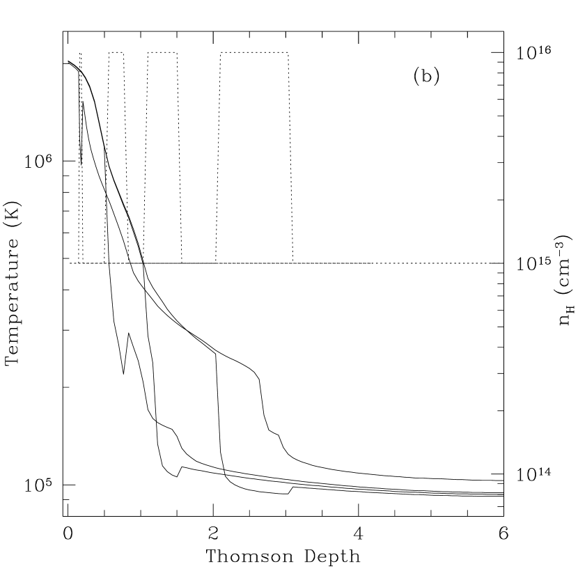
Figure 1: Gas temperature (solid lines) & number density (dotted lines) as a function of $\tau_{\mathrm{T}}$ for eight $\xi=250$ erg cm s^-1 models. (a) Results for the case when $f_{\rho}$=0.1. Steps were placed at $\tau_{\mathrm{step}}=0.1,0.5,1$ & $2$, each with $\Delta\tau=0.5\tau_{\mathrm{step}}$. The gas temperature increases at the position of the drop in density, but otherwise there is little impact in the overall shape of the temperature profile. (b) As in (a), except $f_{\rho}=10$. In this case, the temperature falls at the jump in density, but, because of the increased cooling rates at lower $T$, it does not recover to a similar overall profile.

As an illustration of the technique, Figure 1 plots the temperature and density profiles as a function of $\tau_{\mathrm{T}}$ for eight $\xi=250$ erg cm s^-1 models. The results are shown for $f_{\rho}=0.1$ in Fig. 1(a) and $f_{\rho}=10.0$ in Fig. 1(b). In each plot the dotted lines show the density profiles for four different steps (occurring at $\tau_{\mathrm{step}}=0.1,0.5,1$ & $2$) inserted into the slab, while the solid lines denote the final temperature profile. All the steps shown here have a width of $\Delta\tau=0.5\tau_{\mathrm{step}}$ (i.e., $k=0.5$). The gas temperature reacts as expected: it increases by a factor of few within a density drop, and decreases within a jump. However, the effect of an increase in $n_{\mathrm{H}}$ seems to have a greater impact on the overall temperature profile than a sudden drop in density. Fig. 1(a) shows that outside of the step, the temperature profiles are roughly similar, and indeed closely resembles the one from a constant density model (not shown). On the other hand, Fig. 1(b) shows that the temperature profiles are quite different for the four models. The differences between these two cases illustrates the major difference between an increase or a decrease in density. If the density changes by a factor $f_{\rho}$ then the ionization parameter in that region is changed by $1/f_{\rho}$. When $f_{\rho}<1$, the gas in the altered zones is more easily ionized which raises the temperature, but, most importantly, the recombination and free-free emissivity rates (which scale as $n_{e}^{2}\approx n_{\mathrm{H}}^{2}$) are reduced. It is this increase in cooling when the gas becomes denser which has the largest impact on the temperature profiles seen in Fig. 1(b). However, the ionized gas in a low density region may be a strong emitter in some energy bands (e.g., the 6.7 keV Fe K$\alpha$ line). Furthermore, a decrease in density will also lower the opacity to radiation emitted from below. Therefore, we now turn to see how the impact of a sudden density change impacts the reflection spectrum.

2.2 Results

As a first step in determining the effects of a step in density on the reflection spectrum, we simply overplot the predicted emission with that from a constant density slab under the same illumination conditions. Four examples of this comparison, one for each value of $\xi$, are shown in the upper panels of Figure 2. Since in some cases any differences between the two spectra are difficult to see by eye, we plot in the lower panels the ratio between the constant density and the inhomogeneous model spectra. Prior to the ratio being calculated the $\Gamma=2$ power-law was added to each spectrum so that each had a reflection fraction of unity. This was done in order for the plot to more accurately represent the ratio of two observed spectra (in AGN & GBHCs the power-law continuum is observed along with the reflected emission).

Figure 2, while only showing four examples, does demonstrate a number of useful points. First, although there are changes, the reflection spectra from the toy inhomogeneous models are not dramatically different from the constant density results; that is, they still look qualitatively like the spectra first presented by Ross & Fabian (1993). Secondly, the three variables regarding the density step (its placement, depth/height, and width), as well as the value of $\xi$, all affect the deviations observed in the spectra. For example, the step illustrated in the $\xi=250$ erg cm s^-1 panel of Fig. 2, which corresponds to one of the models shown in Fig. 1(a), results in a negligible change to the reflection spectra above $\sim 0.7$ keV. The only major differences in the reflection spectrum are a decrease in intensity of low-energy Si XI, O V, and C V lines. In this case, the drop in energy was placed too deep into the layer for it to make much difference to the reprocessed emission. However, at larger ionization parameters, the incoming X-rays penetrate further into the slab, and so a step at $\tau_{\mathrm{step}}=1$ can have a large impact on the reflection spectrum. This is seen in the $\xi=500$ erg cm s^-1 panel of Fig. 2, but more dramatically in the $\xi=1000$ erg cm s^-1 plot. In both these cases, the low density step alters the reflection spectra so that they have a shape that resembles ones with a larger value of $\xi$ (less absorption, broader spectral features). These two plots show that the reflection spectra from a inhomogeneous slab can be a mixture of ionization parameters, similar to ones calculated from hydrostatic atmospheres (Ballantyne et al., 2001b). Of course, when the step causes an increase in density, as is shown in the $\xi=125$ erg cm s^-1 panel, then a spectrum typical of a lower ionization parameter (stronger absorption and low-energy emission lines) is mixed in with the results.

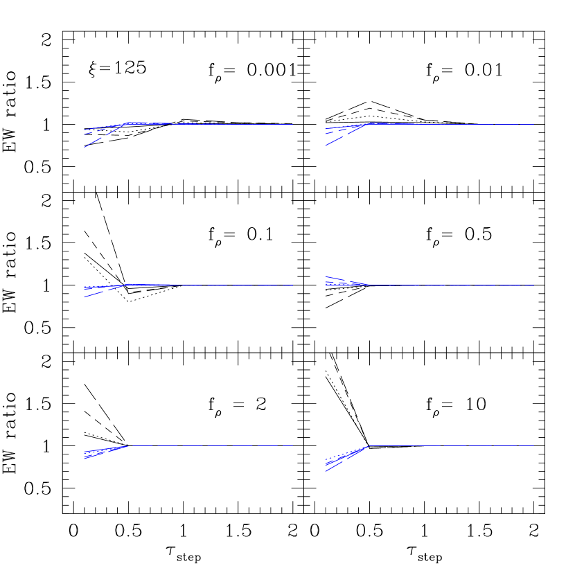
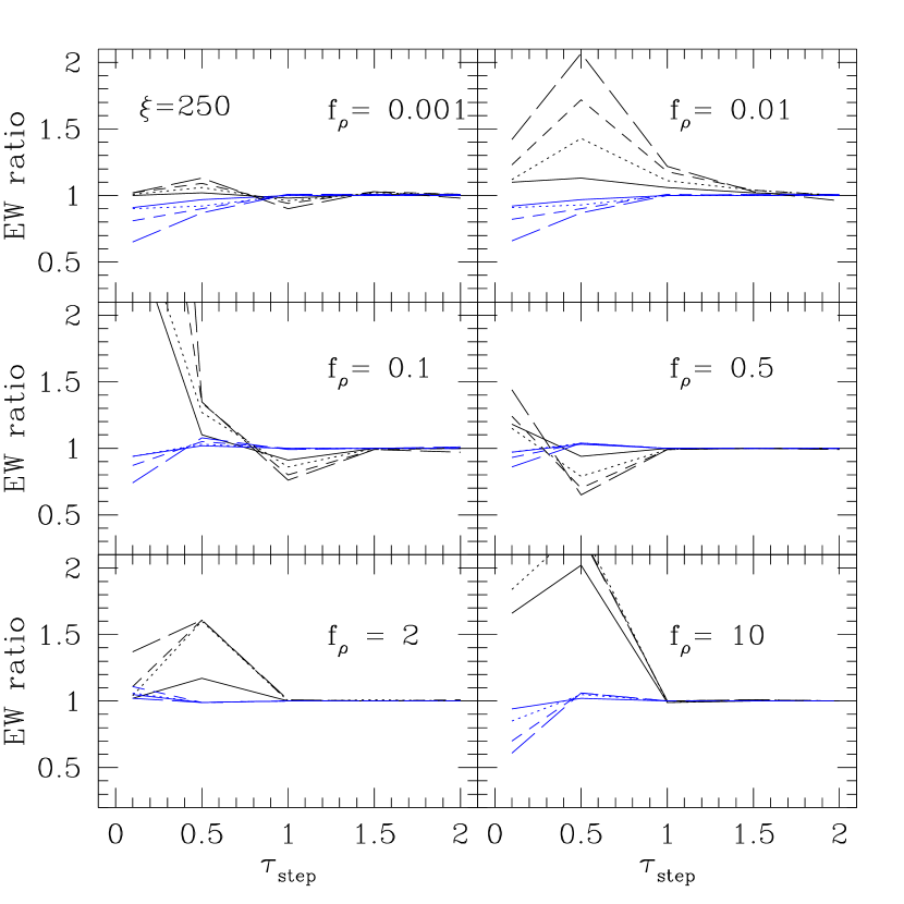
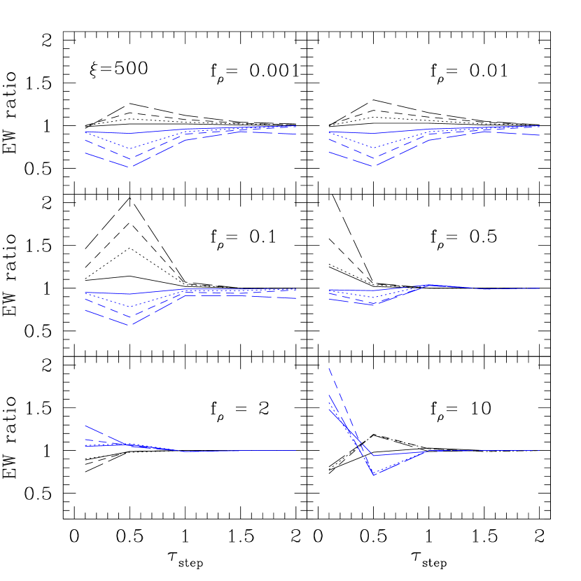
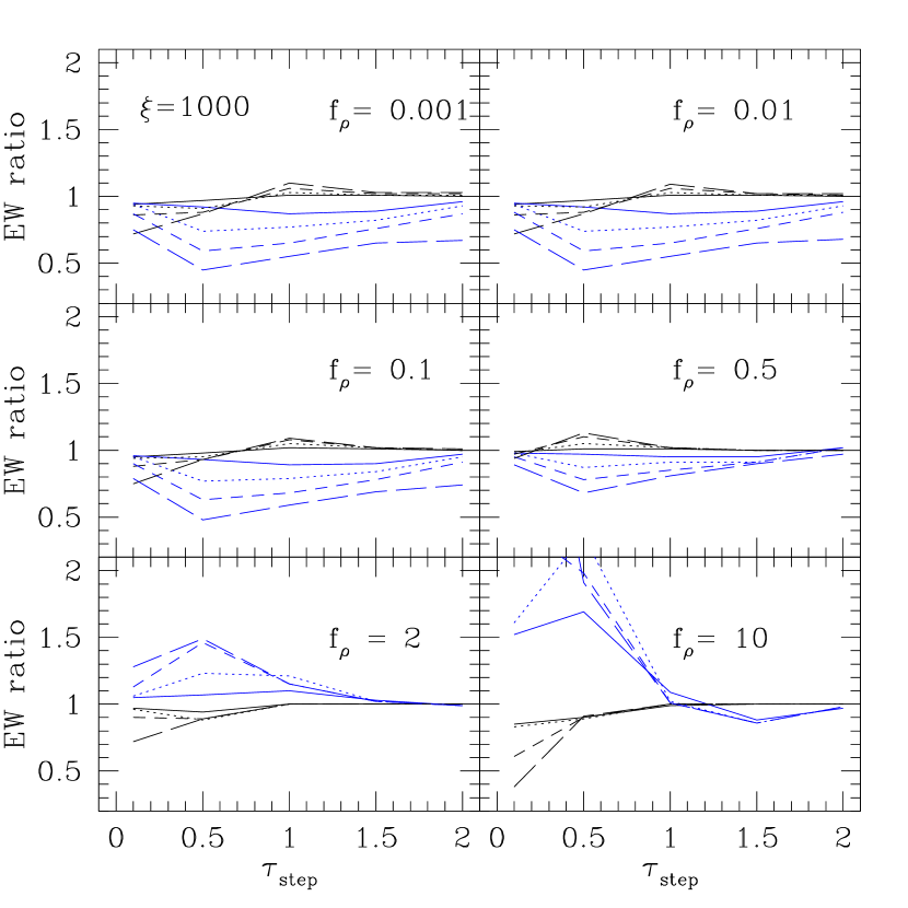
Figure 3: These plots show as a function of $\tau_{\mathrm{step}}$ the ratio of the Fe K$\alpha$ (black) and O viii (blue) Ly$\alpha$ equivelant widths from the toy inhomogeneous models to those from the constant density models. The six panels in each plot descibe the results for each value of $f_{\rho}$, while the linestyles denote the different values of $k$: solid ($k=0.2$), dotted ($k=0.5$), short-dashed ($k=1$) and long-dashed ($k=2$). The EWs were calculated from the total (reflection+incident) spectra. See the text for the discussion.

Although Fig. 2 does show that density inhomogeneities can cause observable effects in the reflection spectra, the results are largely qualitative and selective (there are $\sim 475$ other possible panels). To better quantify the results, and to obtain a more general overview of the parameter space, we calculated the Fe K$\alpha$ and O VIII Ly$\alpha$ EWs from the total (reflected+incident) spectrum for each two-density model and compared it to the values from the corresponding constant density models. The EWs were calculated by integrating the spectrum between 6 and 7 keV for Fe K$\alpha$, and between 0.6 and 0.7 keV for O VIII Ly$\alpha$. Figure 3 shows the results of this exercise, where for each $\xi$ we plot the EW ratio (defined as two-density model/constant density) for both the Fe K$\alpha$ (black) and O VIII (blue) lines as a function of $\tau_{\mathrm{step}}$. Each plot contains 6 panels for the different values of $f_{\rho}$, and the different style of lines within the panel denotes a particular value of $k$. There is plenty of information in this figure, and it is worth going through it in detail, but before doing so there is one general point that can be made. In almost every instance the magnitude of the EW ratio shown in Fig. 3 is proportional to the value of $k$; that is, the wider the step, the greater the change to the reflection spectrum for those values of $f_{\rho}$ and $\tau_{\mathrm{step}}$.

Starting with the $\xi=125$ erg cm s^-1 plot, we find that because of the relatively weak illumination, the density change generally only affects the EWs for $\tau_{\mathrm{step}}<0.5$. The largest changes to the Fe K$\alpha$ EW are when $f_{\rho}=0.1,\,2$ or $10$. In the first case, the increase in EW is due to the appearance of a 6.7 keV component to the Fe K$\alpha$ line, while the later two instances are a result of a stronger 6.4 keV component. The reason why the ionized line appears in the $f_{\rho}=0.1$ models but not in the $f_{\rho}=0.01$ or $0.001$ cases is that the Fe is almost entirely fully stripped in the very low density zones and so does not contribute much emission (as do the other metals). The O VIII EW varies only slightly, except for when $f_{\rho}=10$ where it drops by $\sim 30$% due to a low ionization fraction in the overdense region.

A similar pattern is seen in the $\xi=250$ erg cm s^-1 models, with the changes now occurring for $\tau_{\mathrm{step}}<1$. There are significant variations in the Fe K$\alpha$ EW for most values of $f_{\rho}$, with the largest changes ($>$ factor of 8) occurring in the $f_{\rho}=0.1$ case. The reflection spectrum for the $\xi=250$ erg cm s^-1 constant density model (seen as the dashed line in Fig. 2) has a very weak Fe K$\alpha$ line due to Auger destruction (Ross, Fabian & Brandt, 1996). Therefore, changes to the density which result in either a 6.7 keV line ($f_{\rho}=0.1$) or a strong 6.4 keV line ($f_{\rho}=10$) cause a significant increase in the EW. At this value of $\xi$ it seems to be difficult to increase the O VIII EW by density steps, but it can be lowered by nearly a factor of two when $f_{\rho}=10$.

Increasing the illumination level so that $\xi=500$ erg cm s^-1 results in some changes in the reflected emission with a step down at $\tau_{\mathrm{step}}\sim 2$, but, from Fig. 3, we see that the most substantial changes still occur at $\tau_{\mathrm{step}}\lesssim 0.5$. The Fe K$\alpha$ EW differs significantly from the constant density value only when $f_{\rho}=0.1$ or $0.5$. In these cases the iron in the low density zones becomes highly ionized, but not fully stripped, increasing the column of the He-like species. The line is also broader due to Compton down-scattering. Again, we see that the spectrum takes on the properties of one from a larger $\xi$. This is also reflected in the changes in the O VIII EW, which is much smaller than the constant density model for $f_{\rho}=0.001$–$0.5$. However, the opposite behavior (a larger O VIII EW and a smaller Fe K$\alpha$ EW) is seen when the step causes an increase in density and low-$\xi$ features are mixed into the reflection spectrum. In most of those models, the 6.7 keV Fe line and the O VIII Ly $\alpha$ line are reduced and enhanced in intensity, respectively, although an interesting counter-example is seen when $f_{\rho}=10$ and $\tau_{\mathrm{step}}=0.5$. In this model, the overdense region is placed at a depth so that both a 6.4 keV and a 6.7 keV Fe K$\alpha$ line is emitted, causing an increase in the EW. Similarly, the O VIII EW falls because of a significant transition to O VII emission.

Finally, the most highly ionized runs ($\xi=1000$ erg cm s^-1) show little variation in the Fe K$\alpha$ EW when $f_{\rho}<1$. The only exceptions are when the density deficit is near the surface and the high ionization parameter in these zones decreases the amount of 6.7 keV emitting ions. As a result, the line EW falls by about 25%. On the other hand, when $f_{\rho}=10$, the Fe K$\alpha$ EW can drop by over a factor of two because the overdense region stops the ionization front at a much shallower depth in the slab. The O VIII EW is always smaller than its constant density value when $f_{\rho}<1$, but can increase by over a factor of 2 (up to 110 eV) when there is a density enhancement just beneath the surface.

In summary, we find that toy models which place a top-hat function of variable width and depth into a constant density slab, can produce observable effects on the resulting reflection spectra. Generally the largest impact on the spectrum, as measured by the Fe K$\alpha$ and O VIII EWs, occurs when the step is placed at $\tau_{\mathrm{step}}\sim 0.5$ into the layer. Furthermore, changing the density by only relatively small factors of 2–10 can produce significant effects. The resulting reflection spectra are reminiscent of the one produced by hydrostatic models in so far as they show features from a mixture of ionization parameters.

2.3 Fits with Constant Density Reflection Spectra

The EW ratios shown in Fig. 3 indicate that density inhomogeneities in the surfaces of accretion disks may have an observable effect on their reflection spectra. Those measurements, however, only use a fraction of the information contained in the model spectra. In this section, we take several example reflection spectra calculated from the two-density models and fit them with ones from the constant density models. This method will allow us to quantify any differences between the two scenarios by using all the information over a given energy range. The exercise may also be indicative of how real inhomogeneities will manifest themselves when fitting data with simple models.

We chose models that showed large changes in its Fe K$\alpha$ or O VIII EW from each of the four ionization parameters considered (the exact model parameters are listed in the note to Table 1). Simulated observations were made with these model spectra by using the ’fakeit’ command in xspecv.11.2.0bp (Arnaud, 1996). The canned XMM-Newton EPIC-pn response matrix epn_sw20_sdY9.rmf was used to generate the data assuming an exposure time of 40 ks. As with the EW calculation in the previous section, the incident power-law was added to the reflection spectra so that each simulated spectrum had a reflection fraction, $R$, of unity. Each faked dataset was then fit with a grid of constant density models (calculated with the same version of the reflection code) between 0.2 and 12 keV as well as between 2 and 10 keV. The fit parameters were the photon index $\Gamma$, the ionization parameter $\xi$, the reflection fraction $R$, and an arbitrary normalization. The results are listed in Table 1, and the residuals are shown in Figure 4.

This particular $\xi=125$ erg cm s^-1 model was chosen because the Fe K$\alpha$ EW increased by over a factor of 2 due to the appearance of a 6.7 keV line. In the 0.2–12 keV energy band, the constant density model does a decent job of recovering the ionization parameter, but the value of $R$ is too low. In contrast, the best fit in the 2–10 keV range has a much larger $\xi$ (466 erg cm s^-1) and $R$. Evidently, the spectrum in this energy band mimics one from a more ionized reflector. The residuals to the 0.2–12 keV fit are shown in Fig. 4 and shows that the low value of $R$ is likely due to the overprediction of the O VIII line (as seen in Fig. 3). Moreover, the ionized Fe K$\alpha$ line cannot be accounted for by this low $\xi$. Ignoring the low energy data increases the reflection fraction as the spectrum attempts to account for the enhanced Fe emission. In both cases, the continuum is fit adequately, but the differences in line emission produce significant residuals.

Statistically, the fit to the $\xi=250$ erg cm s^-1 two-density model over the 0.2–12 keV band is much worse than for the previous case. The best fit ionization parameter is lower than the true one, and so overpredicts the strength of the soft emission lines between 0.3 and 0.6 keV (Fig. 4). According to Fig. 3, the Fe K$\alpha$ EW in this two-density model was $\sim$2 times greater than the corresponding constant density model (although at this $\xi$ the EW is only 20 eV), but that the change in the O VIII EW was marginal. Thus, in this case we find that the overdense region lowers the effective ionization parameter of the reflection spectrum, but this is only discernible through a fit to the soft X-ray emission. Indeed, we find a very good and statistically acceptable fit to this two-density model over the 2–10 keV band. The best fit $\xi$ and $R$ are only slightly larger than their true values to account for the enhanced Fe K$\alpha$ line.

The two-density model chosen from the $\xi=500$ erg cm s^-1 suite of calculations is another overdense model with the step appearing at $\tau_{\mathrm{step}}=0.5$ below the surface. As discussed in § 2.2, this model includes both 6.4 and 6.7 keV iron emission lines, as well as a weaker-than-expected O VIII line. Interestingly, this model gives the worst result when fit by the constant density models, with the reduced $\chi^{2}>3$. As in the $\xi=250$ erg cm s^-1 model, the poor fit is caused almost entirely by an overprediction of the soft X-ray spectral features. The majority of the 0.2–12 keV continuum is well fit by an ionized reflector (the best fit $\xi$ is $\sim$630 erg cm s^-1), but the emission lines cannot be accounted for by this model, resulting in the low value of $R$. The overdense region sitting just below the surface of the reflector produces features that cannot be fit by a single-$\xi$ model. The constant density models do a much better job in the 2–10 keV band, where the best fit ionization parameter is nearly exactly the true one. However, the reflection fraction must be lowered to fit the weaker 6.7 keV Fe line. There are still some residuals in this fit between 7 and 8 keV where the overdense region in the two-density model causes additional absorption than what is predicted by the constant density model.

Our final example considers the case where higher-$\xi$ features are mixed into the reflection spectrum. The $\xi=1000$ erg cm s^-1 model used for fitting had a step with a density drop of $f_{\rho}=0.001$ at $\tau_{\mathrm{step}}=0.5$. The lower density material became highly ionized and weakened both the Fe K$\alpha$ and O VIII lines (Fig. 3). The two constant density fits both show the effects of this dilution, as the best fit $\xi$ is greater than the true value and $R<1$. The residuals shown in Fig. 4 show that an overprediction of soft X-ray features is again the cause for the poor fit. There is also a significant difference in the curvature of the two spectra noticeable between 1 and 3 keV. This is caused by the lower absorption in the two-density model which flattens the continuum.

3 Photon Bubbles and Reflection

The idealised two-density models discussed in the previous section show that inhomogeneities in accretion disk atmospheres may affect the reflection spectrum. We next examine reflection from density structures arising in hydrodynamical disk models. Effects of the ionization processes on the density structure are neglected. Nevertheless, the density arrangement is completely novel in terms of reflection calculations, as it is the first to be considered which did not arise from an ad hoc a priori assumption (such as constant density or hydrostatic balance).

The two-density results indicate that the reflection spectrum is affected by inhomogeneities within the outermost few Thomson depths of the disk atmosphere. By contrast, fluctuations resulting from the MRI may be strongest on scales comparable to the disk thickness (Hawley, Gammie & Balbus, 1995; Stone et al., 1996). The effects of photon bubbles are therefore considered instead. The PBI grows most rapidly at short wavelengths (Blaes & Socrates, 2001), and in Shakura-Sunyaev models typically grows fastest in the disk surface layers (N.J. Turner et al. 2004, in preparation). Exploring X-ray reprocessing from photon bubbles is likely to be a good first step toward understanding the reflection properties of radiation-dominated disks.

The photon bubble instability was first discussed by Arons (1992) in the context of accreting magnetized neutron stars, and was shown by Gammie (1998) to occur in the inner, radiation-supported regions of magnetized accretion disks. For magnetic pressures exceeding the gas pressure, and perturbation wavelengths shorter than the gas scale height, the instability operates when disturbances in radiative flux displace gas along field lines, leading to propagating density variations which grow over time. Linear growth is fastest at wavelengths shorter than the gas pressure scale height, but is absent at wavelengths with optical depths much less than unity, as these support no flux variations. An approximate criterion for instability is that photon diffusion carry a greater energy flux than radiation advected at the gas sound speed (Blaes & Socrates, 2003).

Reflection spectra were calculated using a density profile taken from a two-dimensional radiation-MHD simulation of the growth of photon bubbles in a Shakura-Sunyaev model disk. The simulation was carried out with the Zeus MHD code (Stone & Norman, 1992a, b) and its flux-limited radiation diffusion module (Turner & Stone, 2001). Opacities due to electron scattering and bremsstrahlung were included. The domain was a small patch of the disk, centered 34 $R_{\mathrm{S}}$ from a black hole of $10^{8}M_{\odot}$. The patch extended 1.08 Shakura-Sunyaev scale-heights either side of the midplane, and its width was one-quarter of its height. The grid consisted of $64\times 256$ zones. The initial density and temperature profiles were those of a Shakura-Sunyaev model with $\alpha=0.06$, and accretion rate 12% of the Eddington rate for a 10% luminous efficiency. During the simulation, no $\alpha$-viscosity was applied. Differential rotation was neglected, so that the MRI was absent, and the material was allowed to cool by radiative losses. Photons initially diffused from midplane to boundary in nine orbits. The calculation was started with a magnetic field having a pressure 10% of the midplane radiation pressure, and inclined at $45^{\circ}$. After 3.4 orbits, the PBI had developed into trains of propagating shocks, with density contrasts of up to two orders of magnitude. The vertical density profile used in the subsequent reflection calculations was taken from an arbitrary vertical ray, and is shown in the insets to Figure 5.

3.1 Results

As with the two-density models, this new density structure was then irradiated by a power-law ($\Gamma=2$) of X-rays. In this case, there is no unique ionization parameter so instead the models are distinguished by the incident X-ray flux: $F_{\mathrm{X}}=10^{13}$, $2.5\times 10^{13}$, $5\times 10^{13}$, and $10^{14}$ erg cm^-2 s^-1. The Shakura-Sunyaev flux for the assumed disk parameters is $3\times 10^{13}$ erg cm^-2 s^-1. All four models converged, and the resulting reflection spectra are presented in Figure 5. The gas temperature and number density are plotted in the insets to each panel, and illustrates how the temperature structure for each case was affected by the density profile.

The latter three spectra all exhibit strong 6.7 keV emission lines from He-like iron, while, unusually, the most weakly illuminated model produces both a 6.4 and a 6.7 keV line of about equal strength. The rapid drop in density below one Thomson depth causes the surface layers to be easily ionized and able to produce a 6.7 keV emission line even with a relatively small incident flux. On the other hand, the overdense region at $\tau_{\mathrm{T}}\approx 1$ produces a lot of soft X-ray line emission, even for highly illuminated situations. Thus, the emission below $2$ keV is consistently important, despite the incident flux varying by an order of magnitude.

3.2 Fits with Constant Density Reflection Spectra

To quantify any effects the photon bubbles may have on the reflection spectra we fit the models with a grid of constant density spectra. The procedure was exactly the same as with the two-density models in § 2.3: the power-law was added to the photon bubble spectra and then the sum was used as the basis for a 40 ks XMM-Newton simulation. As before, constant density fits were performed in both the 0.2–12 keV and 2–10 keV energy bands. A constant density grid with $n_{\mathrm{H}}=1.4\times 10^{12}$ cm^-3 was used for fitting the photon bubble reflection spectra in order to offset any changes in the reflection spectra due solely to the lower density. The best fit parameters for each value of $F_{\mathrm{X}}$ are listed in Table 2, and the residuals are shown in Figure 7.

The constant density models had difficulty fitting the spectra over the wide 0.2–12 keV energy range, with most of the trouble arising from the soft X-ray lines. The best $\chi^{2}$ was found with the $F_{\mathrm{X}}=10^{13}$ erg cm^-2 s^-1 model, where one ionization parameter seemed to provide a good fit to the spectrum at energies $\gtrsim 0.7$ keV. The best fit $\xi$ was indicative of an ionized slab, and, indeed, the model could not account for the small 6.4 keV line predicted by the spectrum. Despite this problem, the fit was able to recover the correct values of both $\Gamma$ and $R$. The fit had difficulty below 0.5 keV, however, where it overpredicted the emission. This is most likely a result of extra absorption (over that predicted for the fitted $\xi$) due to the density enhancement just beneath the surface in the photon bubble model.

Fits to the remaining three models in this energy band all resulted in reduced $\chi^{2}>2$. A single ionization parameter could not simultaneously account for the shape of the continuum, and the strong soft X-ray and 6.7 keV Fe K$\alpha$ lines. The best fit values of $R$ were always less than the ‘true’ value of unity. In these cases the photon bubble models predicted significant emission from a variety of ionization parameters, so that the resulting spectrum exhibited a mixture of features. As a result, a single ionization parameter fit was not adequate.

The fits to the photon bubble models improved markedly in the 2–10 keV energy band with $\xi$ increasing substantially in order to fit the Fe K$\alpha$ line. As a result, all four fits were statistically acceptable. Except for the $F_{\mathrm{X}}=10^{13}$ erg cm^-2 s^-1 model, the reflection fractions again are still underestimated by the constant density fits with the best fit value of $R$ decreasing with the $F_{\mathrm{X}}$ of the model. A greater than expected amount of absorption is the likely explanation for this effect. The density enhancement at $\tau_{\mathrm{T}}\sim 1$ in the photon bubble model causes more continuum absorption from oxygen then what the reflection models expect (given, e.g., the highly ionized Fe K$\alpha$ line). This enhancement becomes more important as $F_{\mathrm{X}}$ is increased and spectral features are formed both above and below it. The extra absorption decreases the magnitude of the continuum and emission, and thus results in a lower $R$ when fit with the constant density models. Aside from the low value of $R$, reflection from a uniform slab does a good job describing the photon bubble spectra between 2 and 10 keV.

4 Discussion

Currently, the interpretation of the reflection continuum observed in the X-ray spectra of AGN is the primary means to glean information regarding the accretion geometry and its radiative environment. It is therefore vital that the models of reflection, on which such conclusions are based, explore a number of different physical situations which may be relevant to accretion physics. Motivated by the inhomogeneous nature of recent numerical simulations of radiation-dominated accretion disks, we have begun a study of examining the consequences of such density changes to the X-ray reflection spectrum.

Our first results, presented in the previous sections, considered reprocessing from a two-density model, where density steps or jumps were inserted into a uniform slab, and a slice from a PBI simulation. The new reflection spectra were then compared with ones calculated assuming a constant density atmosphere, as these are most frequently used in data analysis. We found that the density inhomogeneities can result in observationally important differences between the two cases. As in models with a hydrostatic atmosphere, the reflection spectra can no longer be described by a single ionization parameter, but exhibit features from a mixture of ionization states. However, while in the hydrostatic case the spectra can be adequately described as a diluted constant density model because of a diffuse hot scattering layer on the surface (Ballantyne et al., 2001b), the inhomogeneous models can show emission from both low and high $\xi$ material simultaneously, depending on the nature of the density change. This gives the spectra a complexity and richness that the hydrostatic models lacked.

The magnitude and characterization of the change in the reflection spectrum depends on both the nature of the inhomogeneity and the strength of the incident X-rays. For the two-density models, where the calculations could be distinguished by the original ionization parameter $\xi$ of the uniform slab, the greatest impact on the Fe K$\alpha$ and O VIII Ly$\alpha$ EWs occurred when $\tau_{\mathrm{step}}\lesssim 1$ for $\xi\lesssim 1000$. For larger ionization parameters, steps deeper into the gas could make an impact. This correlation is not expected to continue indefinitely however. For example, if an atmosphere had a drop in density at $\tau_{\mathrm{T}}\sim 3$ and it was illuminated to the extent that gas was ionized down to this depth, then the additional line emission or absorption caused by the inhomogeneity would be smeared out by Compton scattering while escaping the layer. Thus, a general conclusion seems to be that density inhomogeneities must be within 2 Thomson depths of the surface to have any impact on the reflection spectrum.

However, there must also be a lower-limit to the depth of any density change in the reflecting medium for it to be effective in altering the spectrum. In the extreme case of cold reflection (e.g., $\xi\approx 10$) ionization effects are important only at $\tau_{\mathrm{T}}\leq 0.1$ from the surface. A density inhomogeniety at such a depth would change such a small amount of gas that it would have a negligible effect on the resulting spectrum.

The results of the two-density models also indicate that relatively small changes in density (say, $\delta\rho/\rho\sim$few) can alter the reprocessed emission. Again, this depends on the effective ionization parameter of the layer, but, as was seen in § 3, underdense regions beneath the surface of a moderately irradiated atmosphere can result in a substantial 6.7 keV iron line. But, if that region was underdense but a large amount, such as 100–1000 times lower, then it will be ionized to such an extent that it has very little effect on the outgoing spectrum. Similarly, an overdense region below the surface may enhance the 6.4 keV Fe K$\alpha$ line. Analogous arguments also apply to the soft X-ray emission lines such as O VIII.

How realistic are these requirements on the density inhomogeneities? It certainly appears plausible, even likely, that accretion flows will naturally generate density contrasts greater than a few, especially in the radiation dominated regime where the photon bubble instability can enhance already existing clumpiness. What remains unknown is if the heterogeneous nature of the flow exists to small enough scales that sufficient inhomogeneity remains within a couple of $\tau_{\mathrm{T}}$ from the disk photosphere. Only very high resolution simulations of this region of accretion disks will be able to definitively answer that question.

Assuming for the moment that the inhomogeneities discussed in this paper occur in reality, what are the immediate observational consequences? Perhaps the most interesting result is that the density jumps can cause the Fe K$\alpha$ line to vary in a way that is completely disconnected from the X-ray continuum. One of the most well known puzzling properties of the possible Fe K$\alpha$ ‘disklines’ is their lack of response to the variable continuum (e.g. Chiang et al., 2000). The line flux typically does vary, but it is often not directly correlated with the continuum (Iwasawa et al., 1996; Weaver et al., 2001; Wang et al., 2001; Vaughan & Edelson, 2001; Markowitz et al., 2003; Iwasawa et al., 2003). One very striking example, which was presented by Petrucci et al. (2002), is an XMM-Newton observation of Mkn 841 that was split into two parts, separated by about 15 hours. These authors found that the EW of the narrow Fe K$\alpha$ dropped by $\sim 2$ between the two observations while the continuum changed by $\sim 10$–$20$%. Although, we are not explicitly modeling this source, Fig. 3 shows that density steps in the surface can give rise to exactly such changes in the Fe K$\alpha$ EW, completely independently of the X-ray continuum. A clear way to test if this is the correct model would be to examine the changes of other emission features in the spectrum, but this would require much more sensitive data. The combination of density inhomogeneities with the non-monotonic evolution of the Fe K$\alpha$ EW due to ionization effects (Ballantyne & Ross, 2002) may naturally result in a poor correlation between the observed flux and the Fe K$\alpha$ EW. However, since the observed X-rays must be averaged for many kiloseconds before spectral analysis, which is longer than the timescale for a change in the density inhomogeneities, as well as the the ionization/recombination timescale, a relationship between the line and continuum may still be uncovered, but at a weaker level than what may have been previously expected.

If the density inhomogeneities beneath the photosphere are relatively small in scale, which should be true for thin disks (where $H<R$, and $H$ is the disk scale height and maximum size of any density fluctuations), then any resulting enhancement or change to the Fe K$\alpha$ line would only occur to a narrow part of the overall line profile, which is determined by the illuminating emissivity. Thus, the appearance of narrow Fe K$\alpha$ lines, such as those recently inferred from observations of NGC 3516 (Turner et al., 2002), NGC 7314 (Yaqoob et al., 2003), and Mrk 766 (Turner, Kraemer & Reeves, 2003) could conceivably originate from density inhomogeneities in the disk.

Variable Fe K$\alpha$ lines from turbulent accretion disks have also been considered by Armitage & Reynolds (2003). These authors assumed the line emissivity was proportional to the local integrated magnetic stress in their numerical simulations, as opposed to our method of assuming a constant illumination and a variable density structure. In reality, a mixture of the two effects would be expected to be ongoing, which should be investigated in future work.

The strength of the soft X-ray emission lines are also affected by density inhomogeneities. These lines are one of the dominant sources of cooling for the X-ray heated gas when it reached $\lesssim 10^{6}$ K. Thus, if overdense or underdense regions are introduced into the layer it can alter the rapidity at which the gas cools, thereby changing the emission features. Interestingly, these changes may occur only in the soft band, with little effect at higher energies. Soft X-ray lines, especially the Ly$\alpha$ lines of O VIII, N VII and C VI, have received some attention recently with the claims that they have been observed to be relativistically broadened in the gratings spectra of some Seyfert 1s (Branduardi-Raymont et al., 2001; Mason et al., 2003; Sako et al., 2003). The exact strength of the lines have been the subject to some debate in the literature (Lee et al., 2001; Ballantyne et al., 2002; A.K. Turner et al., 2003), with the difficulties arising because complex warm absorption features must be taken into account in the spectral modeling. The results from the two-density models show that density inhomogeneities can both enhance and diminish the EWs of the soft X-ray lines.

The constant density fits to both the two-density models and the spectra computed from the photon bubble structure resulted mostly in reflection fractions much less than the true value of unity. If one interprets $R$ as a measure of the solid angle subtended by the disk as seen from the X-ray source, then $R<1$ would indicate some form of truncated accretion flow (e.g., Życki, Done & Smith, 1997, 1998, 1999; Done & Życki, 1999; Eracleous, Sambruna & Mushotzky, 2000; Gliozzi, Sambruna & Eracleous, 2003). Correctly interpreting a fitted value of $R$ is fraught with difficulty since fitting neutral reflection models to ionized accretion disks will also give $R<1$ even if $R=1$ (Ballantyne et al., 2001b; Done & Nayakshin, 2001). Here, we have shown that ionized disk models can produce erroneous $R$ values when there are density inhomogeneities. It is therefore important that other arguments be used (e.g., Barrio, Done & Nayakshin, 2003) before drawing conclusions on the accretion geometry from a fitted value of $R$.

5 Conclusions

Our conclusions from this first paper in our study on reflection from heterogeneous accretion disks can be summarized as follows:

1. The reflection spectrum from accretion disks can be altered by clumps or voids in the gas just beneath the photosphere. The effects range from negligible to large and depend on the structure of the inhomogeneity and the illuminating continuum.

2. The greatest effects on the reflected emission for most ionization parameters occurs when the density change is within $\sim 2$ Thomson depth of the surface.

3. The change in density does not have to be large, even an increase or a decrease by a factor of a few can significantly alter the spectrum from that of a constant density model.

4. Density inhomogeneities beneath the disk surface are a possible explanation for the apparent disconnectedness between the Fe K$\alpha$ line and the X-ray continuum.

5. The soft X-ray emission lines (below 1 keV) are more sensitive to the presence of an inhomogeneity than the harder emission.

6. Fitting the spectra produced from models with inhomogeneities with constant density models shows that a mixture of ionization parameters are present, which often results in reflection fractions smaller than unity.

7. Constant density models may still be a good means of parameterizing reflection spectra, but only for energies $\gtrsim 2$ keV. They will have much more difficulty with broadband spectra that cover the soft X-ray lines emitted from the disk. However, in practice this may only be a problem for sources with weak or non-existent warm absorbers.

In Paper 2, we continue our investigation by computing reflection spectra from the predictions of 3-D radiation dominated accretion disk simulations. Future work will also include a consideration of the dynamical effects of the incident X-rays and multi-dimensional reflection.

Table 1: Results of fitting a sample of two-density models with constant density reflection spectra.

				0.2–12 keV						2.0–10 keV
$\xi_{\mathrm{model}}$	$N$			$\Gamma$	$\xi$	$R$	$\chi^{2}$/d.o.f.			$\Gamma$	$\xi$	$R$	$\chi^{2}$/d.o.f.
125	10-23			2.021${}^{+0.004}_{-0.003}$	147$\pm 3$	0.79${}^{+0.01}_{-0.02}$	2672/2358			2.03${}^{+0.01}_{-0.02}$	466${}^{+38}_{-42}$	1.2$\pm 0.2$	1684/1595
250	10-23			2.026${}^{+0.002}_{-0.004}$	190$\pm 3$	0.92${}^{+0.02}_{-0.01}$	4265/2358			2.03$\pm 0.01$	327${}^{+40}_{-42}$	1.1$\pm 0.1$	1590/1595
500	$5\times 10^{-24}$			2.0	631	0.654	7833/2358			2.02$\pm 0.01$	507${}^{+20}_{-33}$	0.88${}^{+0.08}_{-0.09}$	1638/1595
1000	$2\times 10^{-24}$			2.000${}^{+0.004}_{-0.001}$	1244${}^{+12}_{-17}$	0.75$\pm 0.02$	2994/2358			2.03$\pm 0.01$	1282${}^{+170}_{-181}$	0.81$\pm 0.05$	1639/1595

Note. — The step parameters for the two-density model spectra are (a) $\xi=125$, $f_{\rho}=0.1$, $\tau_{\mathrm{step}}=0.1$, $k=2$; (b) $\xi=250$, $f_{\rho}=10$, $\tau_{\mathrm{step}}=0.5$, $k=0.2$; (c) $\xi=500$, $f_{\rho}=10$, $\tau_{\mathrm{step}}=0.5$, $k=1$; (d) $\xi=1000$, $f_{\rho}=0.001$, $\tau_{\mathrm{step}}=0.5$, $k=2$. $N$ is the normalization of the two-density models in xspec. $R$ is the reflection fraction defined as total=incident+$R\times$reflected. $\xi$ is in units of erg cm s^-1. The error-bars are the 2$\sigma$ uncertainty for the parameter of interest. The simulated data were constructed using the XMM-Newton response matrix epn_sw20_sdY9.rmf and assumed an exposure time of 40 ks.

Table 2: Results of fitting the photon bubble reflection spectra with constant density models.

				0.2–12 keV						2.0–10 keV
$F_{\mathrm{X}}$	$N$			$\Gamma$	$\xi$	$R$	$\chi^{2}$/d.o.f.			$\Gamma$	$\xi$	$R$	$\chi^{2}$/d.o.f.
1013	$2\times 10^{-20}$			1.988${}^{+0.030}_{-0.001}$	561${}^{+1}_{-9}$	1.01$\pm 0.01$	4679/2358			2.04$\pm 0.01$	601${}^{+42}_{-40}$	0.96${}^{+0.11}_{-0.10}$	1632/1595
$2.5\times 10^{13}$	10-20			1.950	565	0.798	5821/2358			2.03$\pm 0.01$	1297${}^{+122}_{-92}$	0.73${}^{+0.13}_{-0.04}$	1695/1595
$5\times 10^{13}$	$5\times 10^{-21}$			1.970	593	0.926	6651/2358			2.00$\pm 0.01$	1340${}^{+488}_{-238}$	0.52$\pm 0.03$	1561/1595
1014	$2\times 10^{-21}$			2.029	491	0.611	5995/2358			1.987${}^{+0.007}_{-0.008}$	2679${}^{+334}_{-297}$	0.46$\pm 0.03$	1627/1595

Note. — $N$ is the normalization of the photon bubble models in xspec. $R$ is the reflection fraction defined as total=incident+$R\times$reflected. $\xi$ is in units of erg cm s^-1. $F_{\mathrm{X}}$ is in units of erg cm^-2 s^-1. The error-bars are the 2$\sigma$ uncertainty for the parameter of interest. The simulated data were constructed using the XMM-Newton response matrix epn_sw20_sdY9.rmf and assumed an exposure time of 40 ks.

Figure 2: Four examples of how the reflection spectra computed from the toy models compare with those from unaltered constant density slabs. The top panel of each plot shows the reflection spectra as the solid line with the constant density one denoted by the long-dashed line. The short-dashed line shows the $\Gamma=2$ incident power-law used for both calculations. The lower panel plots the ratio of the two reflection spectra defined as (constant density/two-density model). With AGN the power-law is also observed along with the reflection spectrum, so the $\Gamma=2$ spectrum was added to the reprocessed emission prior to the ratio being calculated (i.e., they both have a reflection fraction of unity). In this way, we are comparing the spectra as they may be observed.

Figure 4: Simulated count spectra and residuals (in units of standard deviations) to fits of four two-density models with constant density reflection spectra. The fit parameters are given in Table 1.

Figure 5: X-ray reflection spectra (solid line) calculated from the outer 10 Thomson depths of a photon bubble simulation. The short-dashed line denotes the $\Gamma=2$ power-law that was incident on the material. The insert shows the gas temperature (solid line) and number density (dashed line) for each model. Of course, the density is the same for each calculation. The different plots show the results for various incident X-ray fluxes: (a) $F_{\mathrm{X}}=10^{13}$ erg cm^-2 s^-1, (b) $F_{\mathrm{X}}=2.5\times 10^{13}$ erg cm^-2 s^-1.

Figure 5 cont: (c) $F_{\mathrm{X}}=5\times 10^{13}$ erg cm^-2 s^-1, (d) $F_{\mathrm{X}}=10^{14}$ erg cm^-2 s^-1.

Figure 7: Simulated count spectra and residuals (in units of standard deviations) of models computed using the density cut from the photon bubble simulation, and then fit with constant density reflection spectra. The fit parameters are given in Table 2.

References

- Armitage & Reynolds (2003) Armitage, P.J., & Reynolds, C.S., 2003, MNRAS, 341, 1041
- Arnaud (1996) Arnaud K.A., 1996, in Jacoby G., Barnes J., eds, Astronomical Data Analysis Software and Systems V, ASP Conf. Ser. Vol. 101, 17
- Arons (1992) Arons, J., 1992, ApJ, 388, 561
- Balbus & Hawley (1991) Balbus, S.A. & Hawley, J.F., 1991, ApJ, 376, 214
- Balbus & Hawley (1998) Balbus, S.A. & Hawley, J.F., 1998, Rev. Mod. Phys., 70, 1
- Ballantyne & Ross (2002) Ballantyne, D.R. & Ross, R.R., 2002, MNRAS, 332, 777
- Ballantyne et al. (2001a) Ballantyne, D.R., Iwasawa, K. & Fabian, A.C., 2001a, MNRAS, 323, 506
- Ballantyne et al. (2001b) Ballantyne, D.R., Ross, R.R. & Fabian A.C., 2001b, MNRAS, 327, 10
- Ballantyne et al. (2002) Ballantyne, D.R., Ross, R.R. & Fabian A.C., 2002, MNRAS, 336, 867
- Ballantyne et al. (2003) Ballantyne, D.R., Vaughan, S. & Fabian, A.C., 2003, MNRAS, 342, 239
- Barrio et al. (2003) Barrio, F.E., Done, C. & Nayakshin, S., 2003, MNRAS, 342, 557
- Begelman (2001) Begelman, M.C., 2001, ApJ, 551, 897
- Begelman (2002) Begelman, M.C., 2002, ApJ, 568, L97
- Bisnovatyi-Kogan & Blinnikov (1977) Bisnovatyi-Kogan, G.S. & Blinnikov, S.I., 1977, A&A, 59, 111
- Blaes & Socrates (2001) Blaes, O. & Socrates, A., 2001, ApJ, 553, 987
- Blaes & Socrates (2003) Blaes, O. & Socrates, A., 2003, ApJ, 596, 509
- Boller et al. (2002) Boller, Th., Fabian, A.C., Sunyaev, R., Trümper, J., Vaughan, S., Ballantyne, D.R., Brandt, W.N., Keil, R. & Iwasawa, K., 2002, MNRAS, 329, L1
- Branduardi-Raymont et al. (2001) Branduardi-Raymont, G., Sako, M., Kahn, S.M., Brinkman, A.C., Kaastra, J.S. & Page, M.J., 2001, A&A, 365, L140
- Chiang et al. (2000) Chiang, J., Reynolds, C.S., Blaes, O.M., Nowak, M.A., Murray, N., Madajski, G., Marshall, H.L. & Magdziarz, P., 2000, ApJ, 528, 292
- Collin et al. (2003) Collin, S., Coupé, S., Dumont, A.-M., Petrucci, P.O. & Różańska, A., 2003, A&A, 400, 437
- De Rosa et al. (2002) De Rosa, A., Piro, L., Fiore, F., Grandi, P., Maraschi, L., Matt, G., Nicastro, F. & Petrucci, P.O., 2002, A&A, 387, 838
- Done & Życki (1999) Done, C. & Życki, P.T., 1999, MNRAS, 305, 457
- Done & Nayakshin (2001) Done, C. & Nayakshin, S., 2001, ApJ, 546, 419
- Dumont et al. (2002) Dumont, A.-M., Czerny, B., Collin, S. & Życki, P.T., 2002, A&A, 387, 63
- Eracleous et al. (2000) Eracleous, M., Sambruna, R. & Mushotzky, R.F., 2000, ApJ, 537, 654
- Fabian et al. (1989) Fabian, A.C., Rees, M.J., Stella, L. & White, N.E., 1989, MNRAS, 238, 729
- Fabian et al. (2000) Fabian, A.C., Iwasawa, K., Reynolds, C.S. & Young, A.J., 2000, PASP, 112, 1145
- Fabian et al. (2002a) Fabian, A.C., Ballantyne, D.R., Merloni, A., Vaughan, S., Iwasawa, K. & Boller, Th., 2002a, MNRAS, 331, 35
- Fabian et al. (2002b) Fabian, A.C., Vaughan, S., Nandra, K., Iwasawa, K., Ballantyne, D.R., Lee, J.C., De Rosa, A., Turner, A. & Young, A.J., 2002b, MNRAS, 335, L1
- Frank et al. (2002) Frank, J., King, A. & Raine, D., 2002, Accretion Power in Astrophysics, 3rd Edition, Cambridge Univ. Press
- Gammie (1998) Gammie, C.F., 1998, MNRAS, 297, 929
- George & Fabian (1991) George, I.M. & Fabian, A.C., 1991, MNRAS, 249, 352
- Gliozzi et al. (2003) Gliozzi, M., Sambruna, R.M. & Eracleous, M., 2003, ApJ, 584, 176
- Hawley et al. (1995) Hawley, J.F., Gammie, C.F. & Balbus, S.A., 1995, ApJ, 440, 742
- Iwasawa et al. (1996) Iwasawa, K., et al., 1996, MNRAS, 282, 1038
- Iwasawa et al. (2003) Iwasawa, K., Lee, J.C., Young, A.J., Reynolds, C.S. & Fabian, A.C., 2003, MNRAS, in press, (astro-ph/0309432)
- Kaspi et al. (2001) Kaspi, S., et al., 2001, ApJ, 554, 216
- Krolik et al. (1981) Krolik, J.H., McKee, C.F. & Tarter C.B., 1981, ApJ, 249, 422
- Lee et al. (2001) Lee, J.C., Ogle, P.M., Canizares, C.R., Marshall, H.L., Schulz, N.S., Morales, R., Fabian, A.C. & Iwasawa, K., 2001, ApJ, 2001, 554, L13
- Lightman & Eardley (1974) Lightman, A.P. & Eardley, D.M., 1974, ApJ, 187, L1
- Longinotti et al. (2003) Longinotti, A.L., Cappi, M., Nandra, K., Dadina, M. & Pellegrini, S., 2003, A&A, 410, 471
- Markowitz et al. (2003) Markowitz, A., Edelson, R. & Vaughan, S., 2003, ApJ, in press (astro-ph/0308312)
- Martocchia et al. (2002) Martocchia, A., Matt, G., Karas, V., Belloni, T. & Feroci, M., 2002, A&A, 387, 215
- Mason et al. (2003) Mason, K.O., et al., 2003, ApJ, 582, 95
- Matt et al. (1991) Matt, G., Perola, G.C. & Piro, L., 1991, A&A, 247, 25
- Matt et al. (1993) Matt, G., Fabian, A.C. & Ross, R.R., 1993, MNRAS, 262, 179
- Matt et al. (1996) Matt, G., Fabian, A.C. & Ross, R.R., 1996, MNRAS, 280, 823
- Miller et al. (2002a) Miller, J.M., et al., 2002a, ApJ, 570, L69
- Miller et al. (2002b) Miller, J.M., et al., 2002b, ApJ, 577, L15
- Miller et al. (2002c) Miller, J.M., et al., 2002c, ApJ, 578, 348
- Miller et al. (2003) Miller, J.M., et al., 2003, ApJ, in press (astro-ph/0307394)
- Morrison & McCammon (1983) Morrison, R. & McCammon, D., 1983, ApJ, 270, 119
- Nandra & Pounds (1994) Nandra, K. & Pounds, K.A., 1994, MNRAS, 268, 405
- Nayakshin & Kallman (2001) Nayakshin, S. & Kallman, T.R., 2001, ApJ, 546, 406
- Nayakshin & Kazanas (2002) Nayakshin, S. & Kazanas, D., 2002, ApJ, 567, 85
- Nayakshin et al. (2000) Nayakshin, S., Kazanas, D. & Kallman, T.R., 2000, ApJ, 537, 833
- Orr et al. (2001) Orr, A., Barr, P., Guainazzi, M., Parmar, A.N. & Young, A.J., 2001, A&A, 376, 413
- Padmanabhan & Yaqoob (2003) Padmanabhan, U. & Yaqoob, T., 2003, in “High Energy Processes and Phenomena in Astrophysics” (IAU Symp. 214), Suzhou, China (astro-ph/0211386)
- Perola et al. (2002) Perola, G.C., Matt, G., Cappi, M., Fiore, F., Guainazzi, M., Maraschi, L., Petrucci, P.O. & Piro, L., 2002, A&A, 389, 802
- Petrucci et al. (2002) Petrucci, P.O., et al., 2002, A&A, 388, L5
- Pounds et al. (1990) Pounds, K.A., Nandra, K., Stewart, G.C., George, I.M. & Fabian A.C., 1990, Nature, 344, 132
- Reynolds (1997) Reynolds, C.S., 1997, MNRAS, 286, 513
- Reynolds & Nowak (2003) Reynolds, C.S. & Nowak, M.A., 2003, Phys. Rep., 377, 389
- Risaliti (2002) Risaliti, G., 2002, A&A, 386, 379
- Ross & Fabian (1993) Ross, R.R. & Fabian, A.C., 1993, MNRAS, 261, 74
- Ross et al. (1996) Ross, R.R., Fabian, A.C. & Brandt, W.N., 1996, MNRAS, 278, 1082
- Ross et al. (1999) Ross, R.R., Fabian, A.C. & Young, A.J., 1999, MNRAS, 306, 461
- Ross et al. (2002) Ross, R.R., Fabian, A.C., & Ballantyne, D.R., 2002, MNRAS, 336, 315
- Różańska et al. (2002) Różańska, A., Dumont, A.-M., Czerny, B. & Collin S., 2002, MNRAS, 332, 799
- Sako et al. (2003) Sako, M., et al., 2003, ApJ, 596, 114
- Shakura & Sunyaev (1973) Shakura, N.I. & Sunyaev, R.A., 1973, A&A, 24, 337
- Shakura & Sunyaev (1976) Shakura, N.I. & Sunyaev, R.A., 1976, MNRAS, 175, 613
- Stone & Norman (1992a) Stone, J.M. & Norman, M.L., 1992a, ApJS, 80, 753
- Stone & Norman (1992b) Stone, J.M. & Norman, M.L., 1992b, ApJS, 80, 791
- Stone et al. (1996) Stone, J.M., Hawley, J.F., Gammie, C.F. & Balbus, S.A., 1996, ApJ, 463, 656
- A.K. Turner et al. (2003) Turner, A.K., Fabian, A.C., Vaughan, S. & Lee, J.C., 2003, MNRAS, in press (astro-ph/0303418)
- Turner & Stone (2001) Turner, N.J. & Stone, J.M., 2001, ApJS, 135, 95
- Turner et al. (2002) Turner, N.J., Stone, J.M. & Sano, T., 2002, ApJ, 566, 148
- N.J. Turner et al. (2003) Turner, N.J., Stone, J.M., Krolik, J.H. & Sano, T., 2003, ApJ, 593, 992
- Turner et al. (2002) Turner, T.J., et al., 2002, ApJ, 574, L123
- Turner et al. (2003) Turner, T.J., Kraemer, S.B. & Reeves, J.N., 2003, ApJ, in press (astro-ph/0310885)
- Vaughan & Edelson (2001) Vaughan, S. & Edelson, R., 2001, ApJ, 548, 694
- Wang et al. (2001) Wang, J.X., Wang, T.G. & Zhou, Y.Y., 2001, ApJ, 549, 891
- Weaver et al. (2001) Weaver, K.A., Gelbord, J. & Yaqoob, T., 2001, ApJ, 550, 261
- Yaqoob et al. (2001) Yaqoob, T., George, I.M., Nandra, K., Turner, T.J., Serlemitsos, P.J. & Mushotzky, R.F., 2001, ApJ, 546, 759
- Yaqoob et al. (2003) Yaqoob, T., George, I.M., Kallman, T.R., Padmanabhan, U., Weaver, K.A. & Turner, T.J., 2003, ApJ, 596, 85
- Życki et al. (1994) Życki, P.T., Krolik, J.H., Zdziarski, A.A. & Kallman, T.R., 1994, ApJ, 437, 597
- Życki, Done & Smith (1997) Życki, P.T., Done, C. & Smith, D.A., 1997, ApJ, 488, L113
- Życki, Done & Smith (1998) Życki, P.T., Done, C. & Smith, D.A., 1998, ApJ, 496, L25
- Życki, Done & Smith (1999) Życki, P.T., Don,e C. & Smith, D.A., 1999, MNRAS, 305, 231