COSMIC RAY SCATTERING BY COMPRESSIBLE MAGNETOHYDRODYNAMIC TURBULENCE

Abstract

Recent advances in understanding of magnetohydrodynamic (MHD) turbulence call for substantial revisions in the picture of cosmic ray transport. In this paper we use recently obtained scaling laws for MHD modes to calculate the scattering frequency for cosmic rays in the ISM. We consider gyroresonance with MHD modes (Alfvénic, slow and fast) and transit-time damping (TTD) by fast modes. We provide calculations of cosmic ray scattering for various phases of interstellar medium with realistic interstellar turbulence driving that is consistent with the velocity dispersions observed in diffuse gas. We account for the turbulence cutoff arising from both collisional and collisionless damping. We obtain analytical expressions for diffusion coefficients that enter Fokker-Planck equation describing cosmic ray evolution. We calculate the scattering rate and parallel spatial diffusion coefficients of cosmic rays for both Alfvénic and fast modes. We conclude that fast modes provides the dominant contribution to cosmic ray scattering for the typical interstellar conditions in spite of the fact that fast modes are subjected to damping. We show that the efficiency of the scattering depends on the plasma $\beta$ since it determines the damping of the fast modes. We also show that the streaming instability is modified in the presence of turbulence.

1 Introduction

Most astrophysical systems, e.g. accretion disks, stellar winds, the interstellar medium (ISM) and intercluster medium are turbulent with an embedded magnetic field that influences almost all of their properties. High conductivity of the astrophysical fluids makes the magnetic fields “frozen in”, and influence fluid motions. The coupled motion of magnetic field and conducting fluid holds the key to many astrophysical processes.

The propagation of cosmic rays (CRs) is affected by their interaction with magnetic field. This field is turbulent and therefore, the resonant interaction of cosmic rays with MHD turbulence has been discussed by many authors as the principal mechanism to scatter and isotropize cosmic rays (Schlickeiser 2002). Although cosmic ray diffusion can happen while cosmic rays follow wandering magnetic fields (Jokipii 1966), the acceleration of cosmic rays requires efficient scattering. For instance, scattering of cosmic rays back into the shock is a vital component of the first order Fermi acceleration (see Longair 1997).

While most investigations are restricted to Alfvén modes propagating along an external magnetic field (the so-called slab model of Alfvénic turbulence), obliquely propagating MHD modes have been included in Fisk et al. (1974) and later studies (Bieber et al. 1988, Pryadko & Petrosian 2000). The problem, however, is that the Alfvénic turbulence considered in their studies is isotropic turbulence, and this contradicts to the modern understanding of MHD turbulence (Goldreich & Shridhar 1995, see Cho, Lazarian & Yan 2002 for a review and references therein).

A recent study (Lerche & Schlickeiser 2001) found a strong dependence of scattering on turbulence anisotropy. Therefore the calculations of CR scattering must be done using a realistic MHD turbulence model. An important attempt in this direction was carried out in Chandran (2000). However, only incompressible motions were considered. On the contrary, ISM is highly compressible. Compressible MHD turbulence has been studied recently (see review by Cho & Lazarian 2003a and references therein). Schlickeiser & Miller (1998) addressed the scattering by fast modes. But they did not consider the damping, which is essential for fast modes. In this paper we discuss in detail the various damping processes which can affect the fast modes. To characterize the turbulence we use the statistics of Alfvénic modes obtained in Cho, Lazarian & Vishniac (2002, henceforth CLV02) and compressible modes obtained in Cho & Lazarian (2002, henceforth CL02, 2003b,c).

Yan & Lazarian (2002) used recent advances in understanding of MHD turbulence (CL02) to describe cosmic ray propagation in the galactic halo. In this paper we undertake a comprehensive study of cosmic ray scattering rates. In $\S$2, we describe the statistics of Alfvénic and compressible turbulence in various conditions, including both high $\beta$ and low $\beta$ cases. In $\S$3, we describe the resonant interactions between the MHD modes and CRs. The scattering by Alfvén modes and fast modes is presented in $\S$4. We apply our results to different phases of ISM, including Galactic halo, hot ionized medium (HIM), warm ionized medium (WIM) and also partially ionized medium. In $\S$5, we describe the streaming instability in the presence of background turbulence. Discussion of our results is provided in $\S$6 while the summary is given in $\S$7.

2 MHD cascade and its damping

2.1 MHD turbulence cascade

A substantial shortcoming of earlier studies was that the crucial element for cosmic ray scattering, namely, MHD turbulence model was taken somewhat ad hoc. The goal of the current paper is to use the recent advances in quantitative description of MHD turbulence to quantify scattering of cosmic rays.

MHD perturbations can be decomposed into Alfvénic, slow and fast waves with well-known dispersion relations (see Alfvén & Fälthmmar 1963). Alfvénic turbulence is considered by many authors as the default model of interstellar magnetic turbulence. This is partially motivated by the fact that unlike compressible modes, the Alfvén ones are essentially free of damping in fully ionized medium (see Ginzburg 1961, Kulsrud & Pearce 1969). Important questions arise. Can the MHD perturbations that characterize turbulence be separated into distinct modes? Can the linear modes be used for this purpose? The separation into Alfvén and pseudo-Alfvén modes is the cornerstone of the Goldreich-Sridhar (1995, henceforth GS95) model of turbulence. This model and the legitimacy of the separation were tested successfully with numerical simulations (Cho & Vishniac 2000; Maron & Goldreich 2001, CLV02). Separation of MHD perturbations in compressible media into fast, slow and Alfvén modes is discussed in GS95, Lithwick & Goldreich 2001, CL02). The actual decomposition of MHD turbulence into Alfvén, slow and fast modes was performed in CL02, Cho & Lazarian (2003, henceforth CL03), who also quantified the intensity of the interaction between different modes (see below).

Turbulence of Alfvén modes is the default model of MHD turbulence for many resources. Other models are considered less important due to damping. However, within an earlier research it was frequently forgotten that, unlike hydrodynamic turbulence, Alfvénic turbulence is anisotropic, with eddies elongated along the magnetic field (see Higdon 1984, Shebalin et al 1983). This happens because it is easier to mix the magnetic field lines perpendicular to the direction of the magnetic field rather than to bend them. The GS95 model describes incompressible Alfvénic turbulence, which formally means that plasma $\beta=P_{gas}/P_{mag}$, the ratio of gas pressure to magnetic pressure is infinitely large. The corresponding scaling can be easily obtained. For instance, calculations in CLV02 prove that motions perpendicular to magnetic field lines are essentially hydrodynamic. As the result, energy transfer rate due to those motions is constant $\dot{E_{k}}\sim v_{k}^{2}/\tau_{k}$, where $\tau_{k}$ is the energy eddy turnover time $\sim(v_{k}k_{\perp})^{-1}$, where $k_{\perp}$ is the perpendicular component of the wave vector $\mathbf{k}$. The mixing motions couple to the wave-like motions parallel to magnetic field giving a critical balance condition, i.e., $k_{\bot}v_{k}\sim k_{\parallel}V_{A}$, where $k_{\parallel}$ is the parallel component of the wave vector $\mathbf{k}$, $V_{A}$ is the Alfvén speed. From these arguments, the scale dependent anisotropy $k_{\parallel}\propto k_{\perp}^{2/3}$and a Kolmogorov-like spectrum for the perpendicular motions $v_{k}\propto k^{-1/3}$ can be obtained (see Lazarian & Vishniac 1999).

It was conjectured in Lithwick & Goldreich (2001) that GS95 scaling should be approximately true for Alfvén and slow modes in moderately compressible plasma. For magnetically dominated, the so-called low $\beta$ plasma, CL02 showed that the coupling of Alfvénic and compressible modes is weak and that the Alfvénic and slow modes follow the GS95 spectrum. This is consistent with the analysis of HI velocity statistics (Lazarian & Pogosyan 2000, Stanimirovic & Lazarian 2001) as well as with the electron density statistics (see Armstrong, Rickett & Spangler 1995). Calculations in CL03 demonstrated that fast modes are marginally affected by Alfvén modes and follow acoustic cascade in both high and low $\beta$ medium. In what follows, we consider both Alfvén modes and compressible modes and use the description of those modes obtained in CL02, CL03 to study CR scattering by MHD turbulence.

The distribution of energy between compressible and incompressible modes depends, in general, on the way turbulence is driven. CL02 and CL03 studied generation of compressible perturbations using random incompressible driving. As the result we obtained an expression that relates the energy in fast $\sim\delta V_{f}^{2}$ and Alfvén $\sim\delta V_{A}^{2}$ modes,

$$(\delta V_{f}/\delta V_{A})^{2}\sim\delta V_{A}\times V_{A}/(V_{A}^{2}+C_{S}^{2}),$$ (1)

where $C_{S}$ is the sound speed. This relation testifies that at large scales incompressible driving can transfer an appreciable part of energy into fast modes. However, at smaller scales the drain of energy from Alfvén to fast modes is marginal. Therefore the cascades evolve without much of cross talk. Naturally a more systematic study of different types of driving is required. In the absence of this, in what follows we assume that equal amounts of energy are transfered into fast and Alfvén modes when driving is at large scales.

At small scales turbulence spectrum is truncated by damping. Various processes can damp the MHD motions (see Appendix A for details). In partially ionized plasma, the ion-neutral collisions are the dominant damping process. In fully ionized plasma, there are basically two kinds of damping: collisional or collisionless damping. Their relative importance depends on the mean free path in the medium (Braginskii 1965),

$$l_{mfp}=v_{th}\tau=6\times 10^{11}(T/8000K)^{2}/n.$$ (2)

If the wavelength is larger than the mean free path, viscous damping dominates. If, on the other hand, the wavelength is smaller than mean free path, then the plasma is in the collisionless regime and collisionless damping is dominant.

To obtain the truncation scale, the damping time $\Gamma_{d}^{-1}$ should be compared to the cascading time $\tau_{k}$. As we mentioned earlier, the Alfvénic turbulence cascades over one eddy turn over time $(k_{\perp}v_{k})^{-1}\sim(k_{\parallel}V_{A})^{-1}$. The cascade of fast modes takes a bit longer:

$$\tau_{k}=\omega/k^{2}v_{k}^{2}=(k/L)^{-1/2}\times V_{ph}/V^{2},$$ (3)

where $V$ is the turbulence velocity at the injection scale, $V_{ph}$ is is the phase speed of fast modes and equal to Alfvén and sound velocity for high and low $\beta$ plasma, respectively (CL02). If the damping is faster than the cascade, the turbulence is truncated. Otherwise, for the sake of simplicity, we ignore the damping and assume that the turbulence cascade is unaffected. As the transfer of energy between Alfvén, slow and fast modes of MHD turbulence is suppressed, we consider different components of MHD cascade independently.

We get the cutoff scale $k_{c}$ by equating the damping rate and cascading rate $\tau_{k}\Gamma_{d}\simeq 1$. Then we check whether it is self-consistent by comparing the $k_{c}$ with the relevant scales, e.g., injection scale, mean free path and the proton gyro-scale.

Damping is, in general, anisotropic, i.e., the linear damping (see Appendix A) depends on the angle between the wavevector ${\bf k}$ and local direction of magnetic field ${\bf B}$. In the typical ISM this happens at the sufficiently small scales where the direction of ${\bf B}$ is well defined (see discussion in the review by Cho, Lazarian & Vishniac 2003).

Note that unless randomization of wave vectors is comparable to the cascading rate the damping scale gets angle-dependent. Consider fast modes, that will be shown to be the most important for cosmic ray scattering. Their non-linear cascading can be characterized by interacting wavevectors ${\bf k}$ that are nearly collinear (see review by Cho, Lazarian & Vishniac 2003). The possible transversal deviation $\delta k$ can be estimated from the uncertainty condition $\delta\omega t_{cas}\sim 1$, where $\delta\omega\sim V_{ph}\delta k(\delta k/k)$. As $t_{cas}\sim 1/k^{4}v_{k}\sim k^{-1/2}$ (see CL02) the $\delta k$ scales as $k^{3/4}$. Therefore the deviation in ${\bf k}$ direction in the course of interactions decreases with the increase of the wavenumber as $\delta k/k\sim k^{-1/4}$, and the number of interactions required to randomize ${\bf k}$ increases as $k^{1/2}$ with the increase of the wavenumber. This means that the randomization of ${\bf k}$ gets marginal for large $k$. In the presence of anisotropic damping this results in anisotropic distribution of fast mode energy at small $k$.

With this input at hand, it is possible to determine the turbulence damping scales for a given medium. For modes in fully ionized medium one should compare the wavelength and mean free path before determining which damping we should apply. However, we are dealing with the turbulence cascade. Therefore, the situation is more complicated: If the mean free path is larger than the turbulence injection scale, we can simply apply the collisionless damping to the whole inertial range of turbulence. In general one should compare the viscous cut off and the mean free path. If the cutoff scale is larger than the mean free path, it shows that the turbulence is indeed cut off by the viscous damping. Otherwise, we neglect the viscous damping and just apply the collisionless damping to the turbulence below the mean free path. By comparing different damping, we find the dominant damping processes for the idealized ISM phases (see table1).

ISM	galactic halo	HIM	WIM	WNM	CNM	MC
T(K)	$2\times 10^{6}$	$1\times 10^{6}$	8000	6000	100	15
n(cm-3)	$10^{-3}$	$4\times 10^{-3}$	0.1	0.4	30	200
$l_{mfp}$(cm)	$4\times 10^{19}$	$2\times 10^{18}$	$6\times 10^{12}$	$8\times 10^{11}$	$3\times 10^{6}$	$10^{4}$
L(pc)	100	100	50	50	50	50
B($\mu$G)	5	2	5	5	5	15
damping	collisionless	collisionless	collisional	neutral-ion	neutral-ion	neutral-ion

Table 1: The parameters of idealized ISM phases and relevant damping. The dominant damping mechanism for turbulence is given in the last line. HIM=hot ionized medium, CNM=cold neutral medium, WNM=warm neutral medium, WIM=warm ionized medium, DC=dark cloud.

2.2 Statistics of fluctuations

Within random-phase approximation, the correlation tensor in Fourier space is (see Schlickeiser & Achatz 1993)

$$<B_{i}(\mathbf{k})B_{j}^{*}(\mathbf{k^{\prime}})>/B_{0}^{2}=\delta(\mathbf{k}-\mathbf{k^{\prime}})M_{ij}(\mathbf{k}),$$

$$<v_{i}(\mathbf{k})B_{j}^{*}(\mathbf{k^{\prime}})>/V_{A}B_{0}=\delta(\mathbf{k}-\mathbf{k^{\prime}})C_{ij}(\mathbf{k}),$$

$$<v_{i}(\mathbf{k})v_{j}^{*}(\mathbf{k^{\prime}})>/V_{A}^{2}=\delta(\mathbf{k}-\mathbf{k^{\prime}})K_{ij}(\mathbf{k}),$$ (4)

where $B_{\alpha,\beta}$, $v_{\alpha,\beta}$ are respectively the magnetic and velocity perturbation associated with the turbulence. For the balanced cascade we consider, i.e., equal intensity of forward and backward modes, $C_{ij}(\mathbf{k})=0$.

The isotropic tensor usually used in the literature is

$$M_{ij}(\mathbf{k})=C_{0}\{\delta_{ij}-k_{i}k_{j}/k^{2}\}k^{-11/3},$$ (5)

The normalization constant $C_{0}$ here can be obtained if the energy input at the scale $L$ is defined. Assuming equipartition $u_{k}=\int dk^{3}\sum_{i=1}^{3}M_{ii}B_{0}^{2}/8\pi\sim B_{0}^{2}/8\pi$, we get $C_{0}=L^{-2/3}/12\pi$. The normalization for the following tensors are obtained in the same way.

The analytical fit to the anisotropic tensor for Alfvén modes, obtained in CLV02 is,

$$\left[\begin{array}[]{c}M_{ij}({\mathbf{k}})\\ K_{ij}({\mathbf{k}})\end{array}\right]=\frac{L^{-1/3}}{6\pi}I_{ij}k_{\perp}^{-10/3}\exp(-L^{1/3}|k_{\parallel}|/k_{\perp}^{2/3}),$$ (6)

where $I_{ij}=\{\delta_{ij}-k_{i}k_{j}/k^{2}\}$ is a 2D tensor in $x-y$ plane which is perpendicular to the magnetic field, $L$ is the injection scale, $V$ is the velocity at the injection scale. Slow modes are passive and similar to Alfvén modes.

According to CL02, fast modes are isotropic and have one dimensional energy spectrum $E(k)\propto k^{-3/2}$. In low $\beta$ medium, the corresponding correlation is (YL02)

$$\left[\begin{array}[]{c}M_{ij}({\mathbf{k}})\\ K_{ij}({\mathbf{k}})\end{array}\right]={\frac{L^{-1/2}}{8\pi}}H_{ij}k^{-7/2}\left[\begin{array}[]{c}\cos^{2}\theta\\ 1\end{array}\right],$$ (7)

where $\theta$ is the angle between $\mathbf{k}$ and $\mathbf{B}$, $H_{ij}=k_{i}k_{j}/k_{\perp}^{2}$ is also a 2D tensor in $x-y$ plane. The factor $\cos^{2}\theta$ represents the projection as magnetic perturbation is perpendicular to $\mathbf{k}$. This tensor is different from that in Schlickeiser & Miller (1998). For isotropic turbulence, the tensor of the form $\propto E_{k}(\delta_{ij}-k_{i}k_{j}/k^{2})$ was obtained to satisfy the condition $\mathbf{k}\cdot\delta\mathbf{B}=0$ (see Schlickeiser 2002). Nevertheless, the fact that $\delta\mathbf{B}$ in fast modes is in the $\mathbf{k}$-$\mathbf{B}$ plane place another constraint on the tensor so that the term $\delta_{ij}$ doesn’t exist.

In high $\beta$ medium, fast modes in this regime are essentially sound modes compressing magnetic field (GS95, Lithwick & Goldreich 2001, CL03). The compression of magnetic field depends on plasma $\beta$. The corresponding x-y components of the tensors are

$$\left[\begin{array}[]{c}M_{ij}({\mathbf{k}})\\ K_{ij}({\mathbf{k}})\end{array}\right]={\frac{L^{-1/2}}{2\pi}}\sin^{2}\theta H_{ij}k^{-7/2}\left[\begin{array}[]{c}\cos^{2}\theta/\beta^{2}\\ 1/\beta\end{array}\right].$$ (8)

The velocity perturbation in high $\beta$ medium is radial, i.e., along $\mathbf{k}$, thus we have the factor $\sin^{2}\theta$ and also $C_{s}^{2}/V_{A}^{2}=2/\beta$ from the magnetic frozen condition $\omega\delta\mathbf{B}\sim\mathbf{k}\times(\mathbf{v}_{k}\times\mathbf{B})$. In high $\beta$ medium, the energy of fast modes are reduced by $V_{A}^{2}/C_{S}^{2}$, this gives another $2/\beta$. We use these statistics to calculate cosmic ray scattering arising from MHD turbulence.

3 Interactions between turbulence and particles

Particles get into resonance with MHD perturbations if the resonant condition is fulfilled, namely, $\omega=k_{\parallel}v\mu+n\Omega$ ($n=\pm 1,2...$), where $\omega$ is the wave frequency, $\Omega=\Omega_{0}/\gamma$ is the gyrofrequency of relativistic particle, $\mu=\cos\xi$, where $\xi$ is the pitch angle of particles.

Basically there are two main types of resonant interactions: gyroresonance acceleration and transit acceleration (henceforth TTD). The latter requires longitudinal motions and it only operates with compressible modes. Gyroresonance occurs when the Doppler shifted frequency of the wave in the particle’s guiding center rest frame $\omega_{gc}=\omega-k_{\parallel}v\mu$ is a multiple of the particle gyrofrequency, and the rotating direction of wave electric vector is the same with the direction for Larmor gyration of particle. For high energy particles, the resonance happens for both positive and negative $n$. TTD happens due to the resonant interaction with parallel magnetic mirror force $-(mv_{\perp}^{2}/2B)\nabla_{\parallel}\mathbf{B}$. For small amplitude modes, particles should be in phase with the wave so as to have a secular interaction with wave (Schlickeiser & Miller 1998). This gives the Cherenkov resonant condition $\omega-k_{\parallel}v_{\parallel}=0$.

We employ quasi-linear theory (QLT) to obtain our estimates. QLT has been proved to be a useful tool in spite of its intrinsic limitations (Schlickeiser & Miller 1998, Miller 1997). For moderate energy cosmic rays, the corresponding resonant scales are much smaller than the injection scale. Therefore the fluctuation on the resonant scale $\delta B\ll B_{0}$ even if they are comparable at the injection scale. QLT disregards diffusion of cosmic rays that follow wandering magnetic field lines (Jokipii 1966) and this diffusion should be accounted separately. If mean magnetic field is larger than the fluctuations at the injection scale, we may say that the QLT treatment we employ defines parallel diffusion. Obtained by applying the QLT to the collisionless Boltzmann-Vlasov equation, the Fokker-Planck equation is generally used to describe the evolvement of the gyrophase-averaged distribution function $f$,

$$\frac{\partial f}{\partial t}=\frac{\partial}{\partial\mu}\left(D_{\mu\mu}\frac{\partial f}{\partial\mu}+D_{\mu p}\frac{\partial f}{\partial p}\right)+\frac{1}{p^{2}}\frac{\partial}{\partial p}\left[p^{2}\left(D_{\mu p}\frac{\partial f}{\partial\mu}+D_{pp}\frac{\partial f}{\partial p}\right)\right],$$

where $p$ is the particle momentum. The Fokker-Planck coefficients $D_{\mu\mu},D_{\mu p},D_{pp}$ are the fundamental physical parameter for measuring the stochastic interactions, which are determined by the electromagnetic fluctuations (Schlickeiser 1993):

Adopting the approach in (Schlickeiser 1993) and taking into account only the dominant interaction at $n=\pm 1$, we can get the Fokker-Planck coefficients (see Appendix B),

$$\left(\begin{array}[]{c}D_{\mu\mu}\\ D_{pp}\end{array}\right)={\frac{\pi\Omega^{2}(1-\mu^{2})}{2}}\int_{k_{min}}^{k_{max}}dk^{3}\delta(k_{\parallel}v_{\parallel}-\omega+\pm\Omega)$$ (11)

$$\left(\begin{array}[]{c}\left(1+\frac{\mu V_{ph}}{v\zeta}\right)^{2}\\ m^{2}V_{A}^{2}\end{array}\right)\left\{(J_{2}^{2}({\frac{k_{\perp}v_{\perp}}{\Omega}})+J_{0}^{2}({\frac{k_{\perp}v_{\perp}}{\Omega}}))\right.$$ (14)

$$\left[\begin{array}[]{c}M_{{\mathcal{RR}}}({\mathbf{k}})+M_{{\mathcal{LL}}}({\mathbf{k}})\\ K_{{\mathcal{RR}}}({\mathbf{k}})+K_{{\mathcal{LL}}}({\mathbf{k}})\end{array}\right]-2J_{2}({\frac{k_{\perp}v_{\perp}}{\Omega}})J_{0}({\frac{k_{\perp}v_{\perp}}{\Omega}})$$ (17)

$$\left.\left[e^{i2\phi}\left[\begin{array}[]{c}M_{{\mathcal{RL}}}({\mathbf{k}})\\ K_{{\mathcal{RL}}}({\mathbf{k}})\end{array}\right]+e^{-i2\phi}\left[\begin{array}[]{c}M_{{\mathcal{LR}}}({\mathbf{k}})\\ K_{{\mathcal{LR}}}({\mathbf{k}})\end{array}\right]\right]\right\},$$ (22)

where $\zeta=1$ for $k_{min}=L^{-1}$, $k_{max}=\Omega_{0}/v_{th}$ corresponds to the dissipation scale, $m=\gamma m_{H}$ is the relativistic mass of the proton, $v_{\perp}$ is the particle’s velocity component perpendicular to $\mathbf{B}_{0}$, $\phi=\arctan(k_{y}/k_{x}),$ ${\mathcal{L}},{\mathcal{R}}=(x\pm iy)/\sqrt{2}$ represent left and right hand polarization.

The delta function $\delta(k_{\parallel}v_{\parallel}-\omega+n\Omega)$ approximation to real interaction is true when magnetic perturbations can be considered static (Schlickeiser 1993). For cosmic rays, $k_{\parallel}v_{\parallel}\gg\omega$ so that the resonant condition is just $k_{\parallel}v\mu+n\Omega=0$. From this resonance condition, we know that the most important interaction occurs at $k_{\parallel}=k_{\parallel,res}=\Omega/v_{\parallel}$. This is generally true except for small $\mu$ (or scattering near $90^{o}$). In this case, these particles move at a speed $v\mu$ close to Alfvén speed along the magnetic field so that we have to take into account the dynamics of the turbulence (Schlickeiser 1993, Bieber, Matthaeus & Smith 1994, Yan & Lazarian 2003).

4 Scattering of cosmic rays

4.1 Scattering by Alfvénic turbulence

As we discussed in $\S$2, Alfvén modes are anisotropic, eddies are elongated along the magnetic field, i.e., $k_{\perp}>k_{\parallel}$. The scattering of CRs by Alfvén modes is suppressed first because most turbulent energy goes to $k_{\perp}$ due to the anisotropy of the Alfvénic turbulence so that there is much less energy left in the resonance point $k_{\parallel,res}=\Omega/v_{\parallel}\sim r_{L}^{-1}$. Furthermore, $k_{\perp}\gg k_{\parallel}$ means $k_{\perp}\gg r_{L}^{-1}$ so that cosmic ray particles have to be interacting with lots of eddies in one gyro period. This random walk substantially decreases the scattering efficiency. Mathematically, this effect is embodied by the Bessel functions in the Fokker-Plank coefficients. We know that the asymptotic expression of Bessel function $J_{n}(x)\sim 1/\sqrt{x}$. So the suppression will be of the order $(\Omega/k_{\perp}v_{\perp})^{\frac{1}{2}}=(k_{\perp}r_{L})^{\frac{1}{2}}$. Noticing that $k_{\perp}v_{\perp}/\Omega=k_{\perp}\tan\xi/k_{\parallel,res}>1$ if the pitch angle $\xi$ is not close to 0, we can simply use the asymptotic form of Bessel function for large argument. Then we can derive an analytical result for Alfvénic turbulence (see Appendix B),

$$\left[\begin{array}[]{c}D_{\mu\mu}\\ D_{pp}\end{array}\right]=\frac{v^{2.5}\cos\xi^{5.5}}{\Omega^{1.5}L^{2.5}\sin\xi}\Gamma[6.5,k_{max}^{-\frac{2}{3}}k_{res}L^{\frac{1}{3}}]\left[\begin{array}[]{c}1\\ m^{2}V_{A}^{2}\end{array}\right],$$ (23)

where $\Gamma[a,z]$ is the incomplete gamma function. The presence of this gamma function in our solution makes our results orders of magnitude larger than those in Chandran (2000) for the most of energies considered. However, the scattering frequency,

$$\nu=2D_{\mu\mu}/(1-\mu^{2}),$$ (24)

are much smaller than the estimates for isotropic and slab model (see Yan & Lazarian 2002). The Alfvén modes are damped in partially ionized medium at scales larger than the resonant scales of moderate energy CRs. As the anisotropy of the Alfvén modes is increasing with the decrease of scales, the interaction with Alfvén modes becomes more efficient for higher energy cosmic rays. When the Larmor radius of the particle becomes comparable to the injection scale, which is likely to be true in the shock region as well as for very high energy cosmic rays in diffuse ISM, Alfvén modes get important.

It’s worthwhile to mention the imbalanced cascade of Alfvén modes (CLV02). Our basic assumption above was that Alfvén modes were balanced, meaning that the energy of modes propagating one way was equal to that in opposite direction. In reality, many turbulence sources are localized so that the modes leaving the sources are more energetic than those coming toward the sources. The energy transfer in the imbalanced cascade occurs at a slower rate, and the Alfvén modes behave more like waves. The scattering by these Alfvén modes is likely to be more efficient. However, as the degree of anisotropy of imbalanced cascade is currently uncertain, and the process will be discussed elsewhere.

4.2 Scattering by fast modes

The contribution from slow modes is no more than that by Alfvén modes since the slow modes have the similar anisotropies and scalings. More promising are fast modes, which are isotropic (CL02). With fast modes there can be two types of resonant interaction: gyroresonance and transit-time damping (TTD) (Schlickeiser & Miller 1998).

Fast modes potentially can scatter CRs by transit-time damping. From the resonant condition $\omega-k_{\parallel}v_{\parallel}\sim 0$, we see that the contribution is mostly from nearly perpendicular propagating modes ($\cos\theta\sim 0$). According to Eq.(4),we see that the corresponding correlation tensor for the magnetic fluctuations $M_{ij}$ are very small, so the contribution from TTD to pitch angle scattering is less important unless the pitch angle is close to $90^{o}$. The advantage of TTD is that it doesn’t have a distinct resonant scale associated with it. The resonant condition only requires $k_{\parallel}/k=V_{ph}/V_{\parallel}$. As the result, TTD is an alternative to scatter low energy CRs whose Larmor radii are below the damping scale of the fast modes. Moreover, TTD can be substantial to the momentum diffusion or acceleration (also known as the second order Fermi acceleration). It can be crucial in some circumstances, e.g., for $\gamma$ ray burst (Lazarian et al. 2003), and super-Alfvénic grain acceleration (Yan & Lazarian 2003).

Here we apply our analysis to the various phases in ISM.

Recent observations (Beck 2001) suggest that the galactic halos are magnetic-dominant, corresponding to low $\beta$ medium. For low $\beta$ medium, we use the tensors given by Eq.(4). For the halo, the collisionless damping is dominant (see Table 1). As we see from Eq.(A2), the damping increases with $\theta$ unless $\theta$ is close to $\pi/2$, which results in $k_{\perp,c}<k_{\parallel,res}$. This means that the fast modes propagating at smaller angle with the magnetic field are less damped. As a result the argument for the Bessel function in Eq.(B20) is $k_{\perp}\tan\xi/k_{\parallel,res}<1$ unless $\xi$ is close to $90^{o}$. So we can take advantage of the anisotropy of the damped fast modes and use the asymptotic form of Bessel function for small argument $J_{n}(x)\simeq(x/2)^{n}/n!$ to obtain the corresponding analytical result for this case (see Appendix B):

$$\left[\begin{array}[]{c}D_{\mu\mu}\\ D_{pp}\end{array}\right]=\frac{\pi(\Omega v\mu)^{0.5}(1-\mu^{2})}{2L^{0.5}}$$ (27)

$$\left[\begin{array}[]{c}(1-(\left(\frac{k_{\perp,c}}{k_{\parallel,res}}\right)^{2}+1)^{-\frac{7}{4}})/7\\ (1-(\left(\frac{k_{\perp,c}}{k_{\parallel,res}}\right)^{2}+1)^{-\frac{3}{4}})m^{2}V_{A}^{2}/3\end{array}\right]$$ (30)

From this equation, we see the key factor is $(k_{\perp,c}/k_{\parallel,res})=\tan\theta_{c}$. As the collisionless damping is a function of $\theta$, the cutoff scale depends also on $\theta$. Put the Eq.(A2) into the relation $\tau_{k}\Gamma_{L}\simeq 1$, we see $\cos^{1.5}\theta_{c}/\sin^{2}\theta_{c}\propto k_{\parallel,res}^{0.5}\propto\gamma^{-0.5}$. Therefore scattering frequency in the halo increases slowly with energy as shown in Fig.1a. For TTD, the contribution is mostly from the nearly perpendicular propagating modes for which the collisionless damping is small (see Eq.A2). Thus the asymptotics of the Bessel function is not applicable. We obtain a numerical solution from Eq.(B49). The contribution of TTD to scattering is much smaller than that of gyroresonance.

Hot ionized medium (HIM) is in high $\beta$ regime and we adopt the tensors given by Eq.(8). The mean free path of the HIM is of the order of parsec and thus the fast modes in this medium are subjected to collisionless damping (see table1). We use Eq.(A4) to get the corresponding damping scale $k_{c}^{-1}=1.3\times 10^{13}\sin^{4/3}\theta/\cos^{2}\theta$cm. Therefore, fast modes become also anisotropic in HIM resulting in $k_{\perp,c}<k_{\parallel,res}$. For CRs with energy $E_{k}\leq 25$GeV, $k_{\parallel,res}>k_{\perp,c}=\sqrt{k_{c}^{2}-k_{\parallel}^{2}}$, so we can use the asymptotics of Bessel function $J_{n}(x)\simeq(x/2)^{n}/n!$ to get an analytical result for gyroresonance in high $\beta$ medium:

$$\left[\begin{array}[]{c}D_{\mu\mu}\\ D_{pp}\end{array}\right]=\frac{2\pi(\Omega v\mu)^{0.5}(1-\mu^{2})}{L^{0.5}}$$ (33)

$$\left[\begin{array}[]{c}(1-\left(\frac{k_{\parallel,res}}{k_{c}}\right)^{7/2})/7\beta^{2}-(1-\left(\frac{k_{\parallel,res}}{k_{c}}\right)^{11/2})/11\beta^{2}\\ (1-\left(\frac{k_{\parallel,res}}{k_{c}}\right)^{3/2})m^{2}V_{A}^{2}/3\beta-(1-\left(\frac{k_{\parallel,res}}{k_{c}}\right)^{7/2})m^{2}V_{A}^{2}/7\beta\end{array}\right],$$ (36)

from which we see the scattering frequency decreases with $k_{\parallel,res}$ and so increases with $E_{k}$. This result agrees well with the numerical solution obtained by Eq.(22) (see Fig.1a). At high energy end, the resonant scales are much larger than the damping scale $k_{c}^{-1}$ so the effect of damping to the scattering curve can be ignored. As a result, the shape of the scattering curve is similar to the case where there is no damping (see Yan & Lazarian 2002). The scattering frequency in this case according to Eq.(22), increases with Larmor frequency $\Omega_{0}/\gamma$ and the resonant scale $k_{res}^{-1}\sim r_{L}$ , which increase with proton energy $E_{k}$. For $E_{k}>1GeV$, $\gamma$ goes nearly linearly with $E_{k}$ so that the scattering frequency decreases due to the $\Omega_{0}/\gamma$ dependence which changes more rapidly.

According to the results in $\S$2, the warm ionized medium (WIM) is also in low $\beta$ but collisional regime. The mean free path $l_{mfp}=6\times 10^{12}$cm (table1), which corresponds to the resonant scale of CRs with energy $\sim 10$GeV. Thus For CRs harder than 10GeV the resonant modes with $k_{\parallel}=\Omega/v_{\parallel}$ are subjected to collisional damping. Since the viscous damping increases with $\theta$, we can apply Eq.(30) to the gyroresonance in WIM as well. As the viscous damping in the low $\beta$ medium scales as $k_{\perp}^{2}$while the cascading rate $\tau_{k}^{-1}\propto k^{0.5}$, we can get $\cos^{1.5}\theta_{c}/\sin^{2}\theta_{c}\propto k_{\parallel,res}^{1.5}\propto\gamma^{-1.5}$ from the truncation condition $\tau_{k}\Gamma_{L}\simeq 1$. Thus according to Eq.(30) the scattering frequency curve in WIM gets steeper (see Fig.1a). For lower energy CRs, the only available modes are those with ${\bf k}$ in a small cone as the residual of the collisional damping at large scales. As a conservative estimate, we adopt the smallest perpendicular viscous cutoff scale $k_{\perp,c}$ above the mean free path to do the calculation. Certainly, the resonant modes corresponding to this energy range of CRs are also affected by collisionless damping. However, the pitch angle of these modes are so small that the collisionless process is marginal (see Eq.(A2)).

In partially ionized medium, the fast modes are severely damped by the ion-neutral damping. The cascade is cut off before the resonant scales for most of the energy range we considered. Indeed, for the parameters chosen, we find that gyroresonance only contribute to the transport of CRs of energy $\geq 0.8$TeV in DC and $>1$TeV for WNM and CNM. Therefore only TTD contributes to the scattering of moderate energy CRs in these media. Since $k_{\perp}v_{\perp}/\Omega\leq k_{c}\tan\xi/k_{\parallel,res}<1$, we can use the asymptotics of Bessel function $J_{n}(x)\simeq(x/2)^{n}/n!$ to get an analytical result for TTD in these media (see Appendix B)

$$\left[\begin{array}[]{c}D_{\mu\mu}\\ D_{pp}\end{array}\right]=\frac{\pi(1-\mu^{4})^{2}k_{c}^{0.5}V_{A}^{2}}{L^{0.5}v\mu^{3}}\left(1-\left(\frac{V_{A}}{v\mu}\right)^{2}\right)^{1.5}\left[\begin{array}[]{c}1\\ (p\mu)^{2}\end{array}\right],$$ (37)

from which we see $D_{\mu\mu}$ is approximately $\propto 1/v$. As $v$ increases with $E_{k}$ when $E_{k}<m_{p}c^{2}\simeq 1$GeV and $\simeq c$ when $E_{k}>1$GeV, the scattering frequency decreases with energy when $E_{k}<1$GeV and keeps nearly a constant at higher energies. As expected, the scattering is much less efficient in partially ionized media because of ion-neutral damping.

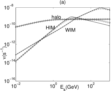
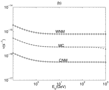
Figure 1: Scattering by fast modes. The scattering frequency $\nu$ given by Eq.(24) vs. (a) the kinetic energy $E_{k}$ of cosmic rays, (b) kinetic energy $E_{k}$ of cosmic rays in partially ionized medium. The solid lines represent our analytical results. In (a), the diamond line is our numerical result for galactic halo, the ’o’ line refers to HIM and the ’x’ line represents WIM. In (b), the diamond line is our numerical result for WNM, the ’o’ line refers to CNM and the ’x’ line represents MC.

From the above results, we see that the fast modes dominate CRs’ scattering in spite of the damping. From Eq.(37), we see the ratio of scattering and momentum diffusion rates $p^{2}D_{\mu\mu}/D_{pp}=1/\mu^{2}$, which means that the scattering and acceleration by TTD are comparable. However, for gyroresonance, we know that $p^{2}D_{\mu\mu}/D_{pp}\sim v^{2}/(min\{\beta,1\}V_{A}^{2})$ (see Eq.(36)and Eq.(30)). Consequently for momentum diffusion (or acceleration) TTD is dominant and the rate differs from the scattering rate by a factor $\sim\mu^{2}$.

A special case is that the cosmic rays propagate nearly perpendicular to the magnetic field, so called the $90^{o}$ scattering problem. The dynamics of the turbulence was suggested to be taken into account in this case (Schlickeiser & Achatz 1993). There have been attempts of using the concept of the dynamical turbulence in dealing with the CR transport before (Bieber et al. 1994). It has been shown in Schlickeiser & Achatz (1993) that if the decay time $\alpha kV_{A}$ is longer, the resonance function can be approximated by $\delta$ function. In other words, $\alpha\rightarrow 0$ is the ”magnetostatic limit”. From (Eq.(3)), we can get $\alpha=(kL)^{-1/2}$. For moderate energy CRs, the corresponding $\alpha<<1$ so that $\delta$ function is still a good approximation even for the $90^{o}$ case. The corresponding resonant scale is $\sim V_{ph}/\Omega$. Thus unlike with Alfvén modes, we can implement unified $\delta$ function and then integrate over the pitch angle $\mu$ to estimate the spatial diffusion. Here we focus on galactic halo since the scattering rate is the highest there. In the precedent calculations, we ignored $V_{ph}$ because it is negligible comparing with $v\mu$. Now $v\mu$ should be replaced with $v\mu\pm V_{ph}$ as seen from the gyroresonance condition $\omega-k_{\parallel}v_{\parallel}=n\Omega$. The complication comes from the cutoff due to damping. As addressed earlier, the fast modes become slab-type at small scales. Thus we can get $\theta_{c}$ from Eq.(3) and Eq.(A4) $k_{\perp,c}/k_{\parallel,res}\simeq\theta_{c}\simeq 2(m_{i}v_{\parallel}/\pi m_{e}\beta\Omega l)^{1/4}\ll 1$. Then we can obtain an analytical solution from Eq.(30) for the parallel spatial diffusion coefficient:

$$\kappa_{\parallel} = \frac{v^{2}}{8}\int_{-1}^{1}d\mu\frac{(1-\mu^{2})^{2}}{D_{\mu\mu}}$$ (38)

$$= \frac{3lv}{4}\left(\frac{m_{e}\beta}{m_{i}\pi}\right)^{0.5}[-1+2\epsilon+2(-1+\epsilon^{2})\ln\frac{\epsilon}{(1+\epsilon)}],$$

where $\epsilon=V_{A}/v$. This result is compared with numerical integral of Eq.(30) in Fig.2b. These results are not applicable to high energy CRs for which the slab-model of fast modes fails.

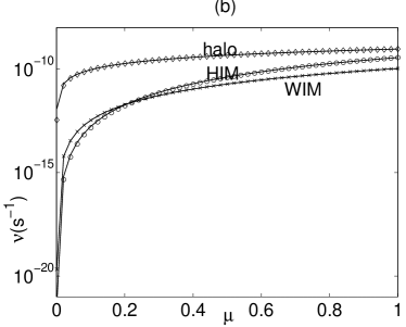
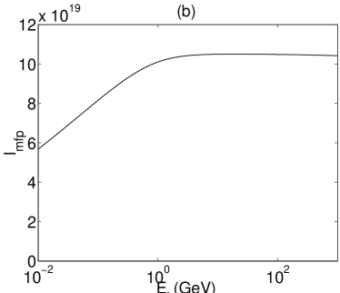
Figure 2: (a)The scattering frequency $\nu$ vs. cosine of pitch angle $\mu$ of 1GeV CR in fully ionized medium. The solid lines represent our analytical results, the diamond line is our numerical result for galactic halo, the ’o’ line refers to HIM and the ’x’ line represents WIM. (b), The mean free path of CRs in galactic halo resulting from numerical integration of Eq.(30)

.

It should be pointed out that all the results above are very much dependent on the plasma $\beta$, which is somewhat uncertain. But the basic conclusion is definite: fast modes dominate the cosmic ray scattering except in very high $\beta$ medium where fast modes are severely damped. This demands a substantial revision of cosmic ray acceleration/propagation theories, and many related problems should be revisited.

5 Cosmic ray self confinement by streaming instability

When cosmic rays stream at a velocity much larger than Alfvén velocity, they can excite resonant MHD modes which in turn scatter themselves. This is so called streaming instability. It was claimed that the instability could provide confinement for cosmic rays with energy less than 100GeV (Cesarsky 1980). However, this was calculated in an ideal regime, namely, there was no background MHD turbulence. Only ambipolar collisional damping was involved. In other words, the self-excited modes would not be damped in fully ionized gas, which is not true for turbulent medium. Here we shall reconsider in turbulent ISM how this instability would affect cosmic ray transport, whether it is still an effective mechanism or not.

The growth rate of the modes of wave number $k$ is given by (Longair 1997)

$$\Gamma(k)=\Omega_{0}\frac{N(\geq E)}{n_{p}}(-1+\frac{v}{V_{A}}),$$ (39a)

where $$N(\geq E) \geq E i.e. v(E)=\Omega/k_{\parallel} n_{p} n(E)\sim 1.6\times 10^{5}(E/ )^{-2.7} N(\geq E)\simeq 0.25\times 10^{-10}(E/ )^{-1.7}$$ is the number density of cosmic rays with energy which resonate with the wave, , , is the number density of charged particles in the medium. If taking the energy spectrum of cosmic ray particles MeV as measured at the Earth (Longair 1997), then GeVcm^-3sr^-1.

The damping rate due to the turbulence cascade depends on the properties of turbulence. To estimate the rate at which background turbulence can suppress th streaming instability we consider both interaction with fast and Alfvénic modes. The interaction with the fast modes happens at the rate $\tau_{k}\sim(k/L)^{-1/2}V_{ph}/V^{2}$ (see Eq.(3)). The interaction with Alfvén modes is less straightforward to quantify because of their anisotropy. Consider the interaction of a perturbation created by streaming particles and the background Alfvénic turbulence. If we approximate this perturbation by a wave with $k=k_{\parallel}$, it gets evident that the interaction will be very different from what takes place between the oppositely moving wave packets in Alfvénic turbulence. If we consider local in ${\bf k}$-space interaction the plane wave created by the streaming instability will undergo random shearing. The mean variation of the phase $\Delta\varphi$ will be approximately $1/\sqrt{N}$, where $N\sim(k_{\perp}/k_{\parallel})^{2}$. The decorrelation time $t_{dc}$ can be estimated using random walk arguments $(\Delta\varphi)^{2}\cdot(t_{dc}\omega)\sim 1$, which provides $t_{dc}\sim\omega^{-1}(k_{\perp}/k_{\parallel})^{2}$.

Thus the dominant damping mechanism here is the cascade of fast modes. By equating the growth rate Eq.((39a)) and the damping rate (Eq.(3)), we can find that the streaming instability is only applicable for particles with energy $<1.5\times 10^{-9}[n_{p}^{-1}(v/V_{A})^{1.5}(L\Omega_{0}/V_{A})^{0.5}]^{1/1.2}$GeV. In HIM, the corresponding energy is $\sim 500$GeV. As shown in the Eq.(39a) , the growth rate depends on the CRs’ density. In those regions where high energy particles are produced, e.g., shock fronts in ISM, $\gamma$ ray burst, SN, the streaming instability is more important.

6 Discussion

We have attempted to apply a realistic model recently obtained for MHD turbulence to the problem of cosmic ray scattering taking into account the turbulence cutoff arising from both collisional and collisionless damping. We considered both gyroresonance and transit-time damping (TTD), and used QLT to obtain our estimates.

In earlier papers it was frequently assumed that Alfvénic turbulence follows Kolmogorov spectrum while the problem of CR scattering was considered. This is incorrect because MHD turbulence is different from hydrodynamic turbulence if magnetic field is dynamically important. Realistic MHD turbulence can be decomposed into, Alfvén, slow and fast modes. They have different statistics (see CL02). The Alfvén and slow modes follow GS95 scalings and show scale-dependent anisotropy. The anisotropy of Alfvén and slow modes reduce the scattering efficiency to such a degree that their impact on cosmic ray propagation is marginal.

Fast modes, however, are promising as a means of scattering due to their isotropy. Even in spite of the damping fast modes dominate scattering if turbulent energy is injected at large scales. We provided calculations for various phases of ISM, including galactic halo, HIM, WIM and partially ionized media. As the fast modes are subjected to different damping processes, the CR scattering varies . In galactic halo and HIM, the fast modes are subjected to collisionless damping. The mean free path in WIM is much smaller, and ion viscosity dominates the damping. All these dampings decrease with $\theta$ and marginal for parallel modes. As the result, the fast modes at small scales become anisotropic with $k_{\parallel}\gg k_{\perp}$. In this sense, fast modes are in slab geometry but with less energies. These modes can efficiently scatter CRs with the resonant scale $k_{\parallel,res}=\Omega/v_{\parallel}$ larger than the cutoff through gyroresonance. TTD is usually weaker for pitch angle scattering than gyroresonance, but dominant for momentum diffusion. In all the cases, the scattering efficiency decreases with plasma $\beta$ because the damping increases with $\beta$ and the perturbations of turbulence decreases with $\beta$.

How good is our model of ISM turbulence? We used spectra for Alfvén and fast modes which follow from theoretical constructions and which were tested numerically (CL02). Within the ISM similar spectra develop dynamically when random driving is applied at large scales (see Mac Low 2003) and therefore we expect that the distribution of energy over scales for different modes to coincide with the assumed ones. The partition of energy over modes depend, however, on driving. For random driving with $\delta V\sim V_{A}$ we expect approximately equal energy in fast and Alfvén modes. As the details of ISM driving are not clear and the QLT provides results correct up to a factor of the order unity, our predictions for fast mode scattering contain an uncertain factor of the order unity. We believe, however, that our results for scattering by Alfvén modes that given by Eq.(23) are subject to more uncertainties related to the turbulence driving. Indeed, the scattering rates that follow from Eq.(23), although orders of magnitude larger than those in Chandran (2000), are still extremely small compared to models with isotropic spectra. Because it is so small, higher order effects may become important. Does the steady state anisotropic spectrum has always enough time to develop? The dynamic establishing of anisotropic spectra of Alfvénic turbulence requires a few eddy turnover times. For imbalanced driving this can take somewhat longer time (see discussion in $\S$5). Therefore one can imagine situations when the spectrum deviates of its steady state form given by Eq. (3). These deviations are most likely to be small. Therefore we do not expect that in typical ISM conditions the contribution of Alfvénic modes is comparable to that of the fast modes. Identification of the particular situations when the opposite may be true requires a more systematic study of particular driving mechanisms and is the subject of future research. We also note, that if energy is injected at the small scales, the anisotropy of the Alfvénic modes is not large and the scattering can be appreciable. The deviations of the spectrum from the steady state one are not important.

Although scattering via fast modes is isotropic at large scales and becomes slab-type at small scales at which damping gets important, our model is radically different from earlier discussed slab and isotropic+slab models (Bieber et al. 1994, Schlickeiser & Miller 1998).We used theoretically motivated models of turbulence that have been tested numerically. Therefore the transitions from one regime to another as well as the values of the intensity of perturbations have good justification within our approach.

We adopted a particular set of parameters of ISM while doing the calculation. The basic conclusion, namely, fast modes dominate the cosmic ray scattering, will remain the same if the parameters are altered. However, since the $\beta$ value in ISM remains uncertain from observation, the damping scale $k_{c}$ is somewhat uncertain. And this determines the energy limit down to which gyroresonance is dominant.

7 Summary

In the paper above we characterized interaction of cosmic rays with balanced interstellar turbulence driven at a large scale. Our results can be summarized as follows:

1. Fast modes provide the dominant contribution to cosmic ray scattering.

2. Scattering of cosmic rays varies from one interstellar phase to another. It sensitively depends on the damping of fast modes.

3. Due to anisotropic plasma damping fast modes develop at small scales anisotropy which makes gyroresonant scattering within slab approximation applicable. At scales where damping is negligible the isotropic gyroresonant scattering approximation is applicable.

4. In partially ionized gas fast modes scatter cosmic rays of energies $\leq 1$TeV by TTD mechanism.

5. Streaming instability is partially suppressed due to the interaction of the emerging magnetic perturbations with the surrounding turbulence.

Appendix A A. Damping of MHD turbulence

Below we summarize the damping processes that we consider in the paper.

Ion-neutral damping

In partially ionized medium, viscosity of neutrals provides damping (see LY02). If the mean free path for a neutral atom, $l_{n}$, in a partially ionized gas with density $n_{tot}=n_{n}+n_{i}$ is much less than the size of the eddies under consideration, i.e. $l_{n}k\ll 1$, the damping time

$$\Gamma_{in}\sim\nu_{n}^{-1}k^{-2}\sim\left(\frac{n_{tot}}{n_{n}}\right)(l_{n}c_{n})^{-1}k^{-2},$$ (A1)

where $\nu_{n}$ is effective viscosity produced by neutrals. The mean free path of a neutral atom $l_{n}$ is influenced both by collisions with neutrals and with ions. The rate at which neutrals collide with ions is proportional to the density of ions, while the rate at which neutrals collide with other neutrals is proportional to the density of neutrals. The drag coefficient for neutral-neutral collisions is $\sim 1.7\times 10^{-10}T$(K)^0.3 cm³ s^-1 (Spitzer 1978), while for neutral-ion collisions it is $\sim{\langle v_{r}\sigma_{in}\rangle}\approx 1.9\times 10^{-9}$ cm³ s^-1 (Draine, Roberge & Dalgarno 1983). Thus collisions with other neutrals dominate for $n_{i}/n_{n}$ less than $\sim 0.09T^{0.3}$. Turbulent motions cascade down till the cascading time is of the order of $t_{damp}$. The maximal damping corresponds to $k^{-1}\sim l_{n}$. If the neutrals constitute less than approximately $5\%$, the cascade goes below $l_{n}$ and is damped at smaller scale (see below).

Collisionless damping

The nature of collisionless damping is closely related to the radiation of charged particles in magnetic field. Since the charged particles can emit plasma modes through acceleration (cyclotron radiation) and Cherenkov effect, they also absorb the radiation under the same condition (Ginzburg 1961). The thermal particles can be accelerated either by the parallel electric field which can also be called Landau damping or the magnetic mirror (TTD) associated with the comoving modes (or under the Cherenkov condition $k_{\parallel}v_{\parallel}=\omega$). The gyroresonance with thermal ions also causes the damping of those modes with frequency close to the ion-cyclotron frequency (Leamon et al. 1998), though it is irrelevant to the low frequency modes since we deal with GeV CRs here. The collisionless damping depends on the plasma $\beta\equiv P_{gas}/P_{mag}$ and the propagation direction of the modes. In general, the damping increases with the plasma $\beta$. And the damping is much more severe for fast modes than for Alfvén modes. For instance, the Alfvén modes are weakly damped even in a high $\beta$ medium, where fast modes are strongly damped. The damping rate $\gamma_{d}=\tau_{d}^{-1}$ of the fast modes of frequency $\omega$ for $\beta\ll 1$ and $\theta\sim 1$ (Ginzburg 1961) is

$$\Gamma_{L} = \frac{\sqrt{\pi\beta}}{4}\omega\frac{\sin^{2}\theta}{\cos\theta}\times[\sqrt{\frac{m_{e}}{m_{H}}}\exp(-\frac{m_{e}}{m_{H}\beta\cos^{2}\theta})$$ (A2)

$$+ 5\exp(-\frac{1}{\beta\cos^{2}\theta})],$$ (A3)

where $m_{e}$ is the electron mass. The exact expression for the damping of fast modes at small $\theta$ was obtained in Stepanov (1958)

$$\Gamma_{L}=\frac{\sqrt{\pi\beta}}{4}\omega\theta^{2}\times\left(1+\frac{\theta^{2}}{\sqrt{\theta^{4}+4\Omega_{i}^{2}/\omega^{2}}}\right)\sqrt{\frac{m_{e}}{m_{H}}}\exp(-\frac{m_{e}}{m_{H}\beta\cos^{2}\theta}).$$

When $\beta\gg 1$, we obtain the damping rate as a function of $\theta$ from Foote & Kulsrud 1979,

$$\Gamma_{L}=\frac{\sin^{2}\theta}{\cos^{3}\theta}\times\cases{2\omega^{2}/\Omega_{i}&for $k<\Omega_{i}/\beta V_{A}$\cr 2\Omega_{i}/\beta&for $k>\Omega_{i}/\beta V_{A}$\cr}$$ (A4)

where $\Omega_{i}$ is the ion gyrofrequency.

Ion viscosity

In a strong magnetic field ($\Omega_{i}\tau_{i}\gg 1$) the transport of transverse momentum is prohibited by the magnetic field. Thus transverse viscosity $\eta_{\perp}$ is much smaller than longitudinal viscosity $\eta_{0}=0.96n(T/eV)\tau_{i}$, $\eta_{\perp}\sim\eta_{0}/(\Omega_{i}\tau_{i})^{2}$. The heat generated by this damping is $Q_{vis}=\eta_{0}(\partial v_{x}/\partial x+\partial v_{y}/\partial y-2\partial v_{z}/\partial z)^{2}/3$, where $v_{x}$, $v_{y}$, $v_{z}$ are the velocity components of the wave perturbation (Braginskii 1965). From the expression, we see that the viscous damping is not important unless there is compression. Therefore Alfvén modes is marginally affected by the ion viscosity.

While the damping due to compression along the magnetic fields can be easily understood, it is counterintuitive that the compression perpendicular to the magnetic also results in damping through longitudinal viscosity. Following Braginskii (1965), the damping of perpendicular motion may be illustrated in the following way. To understand the physics of such a damping, consider fast modes in low $\beta$ medium. In this case, the motions are primarily perpendicular to the magnetic field so that $\partial v_{x}/\partial x=\dot{n}/n\sim\dot{B}/B$. The transverse energy of the ions increases because of the conservation of adiabatic invariant $v_{\perp}^{2}/B$. If the rate of compression is faster than that of collisions, the ion distribution in the momentum space is bound to be distorted from the Maxwellian isotropic sphere to an oblate spheroid with the long axis perpendicular to the magnetic field. As a result, the transverse pressure gets greater than the longitudinal pressure by a factor $\tau_{i}\sim\dot{n}/n$, resulting in a stress $\sim p\tau_{i}\dot{n}/n\sim\eta_{0}\partial v_{x}/\partial x$. The restoration of the equilibrium increases the entropy and causes the dissipation of energy with a damping rate $\Gamma_{ion}=k_{\perp}^{2}\eta_{0}/6\rho_{i}$ (Braginskii 1965).

In high $\beta$ medium, the velocity perturbations are radial as pointed out in $\S 2$. Thus $Q_{vis}=\eta_{0}(k_{x}v_{x}+k_{y}v_{y}-2k_{z}v_{z})^{2}/3=\eta_{0}k^{2}v^{2}(\sin^{2}\theta-2\cos^{2}\theta)^{2}/3$. Dividing this by the total energy associated with the fast modes $E_{k}=\rho_{i}v^{2}$, we can obtain the damping rate $\Gamma_{ion}=k^{2}\eta_{0}(1-3\cos^{2}\theta)^{2}/6\rho_{i}$.

All in all,

$$\Gamma_{ion}=\cases{k_{\perp}^{2}\eta_{0}/6\rho_{i}&for $\beta\ll 1$\cr k^{2}\eta_{0}(1-3\cos^{2}\theta)^{2}/6\rho_{i}&for $\beta\gg 1$\cr}$$ (A5)

Resistive damping

In the paper we ignore the resistive damping because of the following reason. The resistivity is much smaller than the longitudinal ion viscosity for fast modes. For parallel propagating fast modes which are not subjected to the viscous damping from the longitudinal viscosity, the resistive damping scale can be obtained by equating the damping rate $c^{2}k^{2}/8\pi\sigma_{\perp}$ with the cascading rate of the fast modes, where $\sigma_{\perp}\simeq 10^{13}(T/eV)^{3/2}$ (see Kulsrud & Pearce 1969) is the conductivity perpendicular to the magnetic field: $k_{res}^{-1}=1.8\times 10^{7}(L/pc)^{1/3}(T/10^{4}K)^{-1}(V_{A}/kms^{-1})^{-2/3}$cm. This scale turns out to be much smaller than the mean free path, where collisionless damping takes over. For Alfvén modes, the resistive damping rate is $\Gamma_{res}=c^{2}k_{\perp}^{2}/8\pi\sigma_{\parallel}$ (the term associated with $k_{\parallel}$is negligible because of anisotropy), where $\sigma_{\parallel}=1.96\sigma_{\perp}$is the conductivity parallel to the magnetic field. By equating it with the cascading rate of Alfvén modes, we can get the resistive damping scale $k_{res}^{-1}\simeq L(c^{2}/8\pi\sigma_{\parallel}V_{A}L)^{3/4}$. Comparing with the proton Larmor radius, we find $k_{res}^{-1}/r_{L}=3.6\times 10^{-3}(L/pc)^{1/4}(T/10^{4}K)^{-3/2}n^{1/2}(V_{A}/C_{s})^{1/4}$. It’s clear that in many astrophysical plasmas the resistive scale is less than proton Larmor radius, where Alfvén modes can not proceed further because of anomalous resistivity. All in all, we see that the damping arising from resistivity is marginal.

Appendix B B. Fokker-Planck coefficients

In quasi-linear theory (QLT), the effect of MHD modes is studied by calculating the first order corrections to the particle orbit in the uniform magnetic field, and the ensemble-averaging over the statistical properties of the MHD modes (Jokipii 1966, Schlickeiser & Miller 1998). Obtained by applying the QLT to the collisionless Boltzmann-Vlasov equation, the Fokker-Planck equation is generally used to describe the evolvement of the gyrophase-averaged particle distribution. The Fokker-Planck coefficients $D_{\mu\mu},D_{\mu p},D_{pp}$ are the fundamental physical parameter for measuring the stochastic interactions, which are determined by the electromagnetic fluctuations:

$\begin{array}[]{cc}<B_{\alpha}(\mathbf{k})B_{\beta}^{*}(\mathbf{k^{\prime}})>=\delta(\mathbf{k}-\mathbf{k^{\prime}})P_{\alpha\beta}(\mathbf{k})&<B_{\alpha}(\mathbf{k})E_{\beta}^{*}(\mathbf{k^{\prime}})>=\delta(\mathbf{k}-\mathbf{k^{\prime}})T_{\alpha\beta}(\mathbf{k})\\ <E_{\alpha}(\mathbf{k})B_{\beta}^{*}(\mathbf{k^{\prime}})>=\delta(\mathbf{k}-\mathbf{k^{\prime}})Q_{\alpha\beta}(\mathbf{k})&<E_{\alpha}(\mathbf{k})E_{\beta}^{*}(\mathbf{k^{\prime}})>=\delta(\mathbf{k}-\mathbf{k^{\prime}})R_{\alpha\beta}(\mathbf{k}),\end{array}$

Adopting the approach in Schlickeiser & Achatz (1993), we can get the Fokker-Planck coefficients,

$$\left[\begin{array}[]{c}D_{\mu\mu}\\ D_{\mu p}\\ D_{pp}\end{array}\right] = {\frac{\Omega^{2}(1-\mu^{2})}{2B_{0}^{2}}}{\mathcal{R}}e\sum_{n=-\infty}^{n=\infty}\int_{\bf k_{min}}^{\bf k_{max}}dk^{3}\left[i\begin{array}[]{c}\left(1+\frac{\mu V_{A}}{v\zeta}\right)^{2}\\ \left(1+\frac{\mu V_{A}}{v\zeta}\right)mc\\ m^{2}c^{2}\end{array}\right]\int_{0}^{\infty}dte^{-i(k_{\parallel}v_{\parallel}-\omega+n\Omega)t}\left\{J_{n+1}^{2}({\frac{k_{\perp}v_{\perp}}{\Omega}})\left[\begin{array}[]{c}P_{{\mathcal{RR}}}({\mathbf{k}})\\ T_{{\mathcal{RR}}}({\mathbf{k}})\\ R_{{\mathcal{RR}}}({\mathbf{k}})\end{array}\right]\right.$$ (B10)

$$+ J_{n-1}^{2}({\frac{k_{\perp}v_{\perp}}{\Omega}})\left[\begin{array}[]{c}P_{{\mathcal{LL}}}({\mathbf{k}})\\ -T_{{\mathcal{LL}}}({\mathbf{k}})\\ R_{{\mathcal{LL}}}({\mathbf{k}})\end{array}\right]+J_{n+1}({\frac{k_{\perp}v_{\perp}}{\Omega}})J_{n-1}({\frac{k_{\perp}v_{\perp}}{\Omega}})\left.\left[e^{i2\phi}\left[\begin{array}[]{c}-P_{{\mathcal{RL}}}({\mathbf{k}})\\ T_{{\mathcal{RL}}}({\mathbf{k}})\\ R_{{\mathcal{RL}}}({\mathbf{k}})\end{array}\right]+e^{-i2\phi}\left[\begin{array}[]{c}-P_{{\mathcal{LR}}}({\mathbf{k}})\\ -T_{{\mathcal{LR}}}({\mathbf{k}})\\ R_{{\mathcal{LR}}}({\mathbf{k}})\end{array}\right]\right]\right\}$$ (B20)

where $|{\bf k_{min}}|=k_{min}=L^{-1}$, $|{\bf k_{max}}|=k_{max}$ corresponds to the dissipation scale, where $\zeta=1$ for Alfvén modes, $dk^{3}=2\pi k_{\perp}dk_{\perp}dk_{\parallel}$, and $\zeta=k_{\parallel}/k$ for fast modes, $m=\gamma m_{H}$ is the relativistic mass of the proton, $v_{\perp}$ is the particle’s velocity component perpendicular to $\mathbf{B}_{0}$, $\phi=\arctan(k_{y}/k_{x}),$ ${\mathcal{L}},{\mathcal{R}}=(x\pm iy)/\sqrt{2}$ represent left and right hand polarization. For low frequency MHD modes, we have from Ohm’s Law $\mathbf{E}(\mathbf{k})=-(1/c)\mathbf{v}(\mathbf{k})\times\mathbf{B}_{0}$. So we can express the electromagnetic fluctuations $T_{ij},R_{ij}$ in terms of correlation tensors $K_{ij}$. The particular dispersion relations for $\omega$ are not important unless scattering happens at an angle close to $90^{o}$.For $\omega$ we use dispersion relations $\omega=k_{\parallel}V_{A}$ for Alfvén modes and $\omega=kV_{ph}$ for fast modes. Those dispersion relations were used to decompose and study the evolutions of MHD modes in CL02.

For gyroresonance, the dominant interaction is the resonance at $n=\pm 1$. By integrating over $\tau$, we obtain

$$\left(\begin{array}[]{c}D_{\mu\mu}\\ D_{\mu p}\\ D_{pp}\end{array}\right) = {\frac{\pi\Omega^{2}(1-\mu^{2})}{2}}\int_{\bf k_{min}}^{\bf k_{max}}dk^{3}\delta(k_{\parallel}v_{\parallel}-\omega+\pm\Omega)\left(\begin{array}[]{c}\left(1+\frac{\mu V_{ph}}{v\zeta}\right)^{2}\\ \left(1+\frac{\mu V_{ph}}{v\zeta}\right)mV_{A}\\ m^{2}V_{A}^{2}\end{array}\right)$$ (B31)

$$\left\{(J_{2}^{2}({\frac{k_{\perp}v_{\perp}}{\Omega}})+J_{0}^{2}({\frac{k_{\perp}v_{\perp}}{\Omega}}))\left[\begin{array}[]{c}M_{{\mathcal{RR}}}({\mathbf{k}})+M_{{\mathcal{LL}}}({\mathbf{k}})\\ -C_{{\mathcal{RR}}}({\mathbf{k}})-C_{{\mathcal{LL}}}({\mathbf{k}})\\ K_{{\mathcal{RR}}}({\mathbf{k}})+K_{{\mathcal{LL}}}({\mathbf{k}})\end{array}\right]\right.$$

$$- 2J_{2}({\frac{k_{\perp}v_{\perp}}{\Omega}})J_{0}({\frac{k_{\perp}v_{\perp}}{\Omega}})\left.\left[e^{i2\phi}\left[\begin{array}[]{c}M_{{\mathcal{RL}}}({\mathbf{k}})\\ -C_{{\mathcal{RL}}}({\mathbf{k}})\\ K_{{\mathcal{RL}}}({\mathbf{k}})\end{array}\right]+e^{-i2\phi}\left[\begin{array}[]{c}M_{{\mathcal{LR}}}({\mathbf{k}})\\ -C_{{\mathcal{LR}}}({\mathbf{k}})\\ K_{{\mathcal{LR}}}({\mathbf{k}})\end{array}\right]\right]\right\}.$$ (B38)

For TTD,

$$\left(\begin{array}[]{c}D_{\mu\mu}\\ D_{\mu p}\\ D_{pp}\end{array}\right) = {\frac{\pi\Omega^{2}(1-\mu^{2})}{2}}\int_{\bf k_{min}}^{\bf k_{max}}dk^{3}\delta(k_{\parallel}v_{\parallel}-\omega)\left(\begin{array}[]{c}\left(1+\frac{\mu V_{ph}}{v\zeta}\right)^{2}\\ \left(1+\frac{\mu V_{ph}}{v\zeta}\right)mV_{A}\\ m^{2}V_{A}^{2}\end{array}\right)$$ (B49)

$$2J_{1}^{2}({\frac{k_{\perp}v_{\perp}}{\Omega}})\left[\begin{array}[]{c}M_{{\mathcal{RR}}}({\mathbf{k}})+M_{{\mathcal{LL}}}({\mathbf{k}})+e^{i2\phi}M_{{\mathcal{RL}}}({\mathbf{k}})+e^{-i2\phi}M_{{\mathcal{LR}}}({\mathbf{k}})\\ -C_{{\mathcal{RR}}}({\mathbf{k}})-C_{{\mathcal{LL}}}({\mathbf{k}})-e^{i2\phi}C_{{\mathcal{RL}}}({\mathbf{k}})-e^{-i2\phi}C_{{\mathcal{LR}}}({\mathbf{k}})\\ K_{{\mathcal{RR}}}({\mathbf{k}})+K_{{\mathcal{LL}}}({\mathbf{k}})+e^{i2\phi}K_{{\mathcal{RL}}}({\mathbf{k}})+e^{-i2\phi}K_{{\mathcal{LR}}}({\mathbf{k}})\end{array}\right]$$

Define the integrands

$$G(\mathbf{k}) = (J_{2}^{2}({\frac{k_{\perp}v_{\perp}}{\Omega}})+J_{0}^{2}({\frac{k_{\perp}v_{\perp}}{\Omega}}))(K_{{\mathcal{RR}}}({\mathbf{k}})+K_{{\mathcal{LL}}}({\mathbf{k}}))-2J_{2}({\frac{k_{\perp}v_{\perp}}{\Omega}})J_{0}({\frac{k_{\perp}v_{\perp}}{\Omega}})(e^{i2\phi}K_{{\mathcal{RL}}}({\mathbf{k}})+e^{-i2\phi}K_{{\mathcal{LR}}}({\mathbf{k}}))$$

$$T(\mathbf{k}) = 2J_{1}^{2}({\frac{k_{\perp}v_{\perp}}{\Omega}})((K_{{\mathcal{RR}}}({\mathbf{k}})+K_{{\mathcal{LL}}}({\mathbf{k}})+2J_{2}({\frac{k_{\perp}v_{\perp}}{\Omega}})J_{0}({\frac{k_{\perp}v_{\perp}}{\Omega}})(e^{i2\phi}K_{{\mathcal{RL}}}({\mathbf{k}})+e^{-i2\phi}K_{{\mathcal{LR}}}({\mathbf{k}}))$$ (B50)

. We shall show below how they can be simplified in various cases to enable an analytical evaluation of the integral. The spherical components of the correlation tensors are obtained in the following.

For Alfvén modes, their tensors are proportional to

$$I_{ij}=\left(\begin{array}[]{cc}\sin^{2}\phi&-\cos\phi\sin\phi\\ -\cos\phi\sin\phi&\cos^{2}\phi\end{array}\right).$$

Thus we get

$$I_{{\mathcal{RR}}}=I_{{\mathcal{LL}}}={\frac{(I_{x}-iI_{y})}{\sqrt{2}}}{\frac{(I_{x}^{*}+iI_{y}^{*})}{\sqrt{2}}}={\frac{1}{2}}(I_{xx}+I_{yy})={\frac{1}{2}},$$

and

$$e^{i2\phi}I_{{\mathcal{RL}}}+e^{-i2\phi}I_{{\mathcal{LR}}} = {\frac{(I_{x}-iI_{y})^{2}}{2}}\times e^{i2\phi}+{\frac{(I_{x}+iI_{y})^{2}}{2}}\times e^{-i2\phi}=(I_{xx}-I_{yy})\cos 2\phi+(I_{xy}+I_{yx})\sin 2\phi=-1.$$

For Alfvén modes, $k_{\perp}v_{\perp}/\Omega\gg 1$ because of the anisotropy. So we can use the asymptotics of the Bessel function $J_{n}(x)=\sqrt{2/\pi x}\cos(x-n\pi/2-\pi/4)$ when $x\rightarrow\infty$. Thus from Eq.(6,B,B), we simplify the integrand in Eq.(22), $G({\mathbf{k}})\propto k_{\perp}^{-16/3}\exp(-L^{1/3}|k_{\parallel}|/k_{\perp}^{2/3}),$ the integral of which will be $\propto(|k_{\parallel}|L^{1/3})^{-6.5}\Gamma[6.5,k_{max}^{-2/3}|k_{\parallel}|L^{1/3}]$. Then from Eq.(22) we can get the analytical result for the scattering by Alfvén modes as given in Eq.(23).

For fast modes, their tensors have such a component

$$H_{ij}=Ak^{-3.5}\left(\begin{array}[]{cc}\cos^{2}\phi&\cos\phi\sin\phi\\ \cos\phi\sin\phi&\sin^{2}\phi\end{array}\right)$$ . (B53)

Thus we have

$$H_{{\mathcal{RR}}}=H_{{\mathcal{LL}}} = {\frac{1}{2}}(H_{xx}+H_{yy})=\frac{1}{2}$$ (B54)

and

$$e^{i2\phi}H_{{\mathcal{RL}}}+e^{-i2\phi}H_{{\mathcal{LR}}} =(H_{xx}-H_{yy})\cos 2\phi+(H_{xy}+H_{yx})\sin 2\phi=1.$$ (B55)

In general, it’s more difficult to solve the integral in Eq.(B20) for the fast modes because they are isotropic. However, if taking into account damping, Bessel function can be evaluated using the zeroth order approximation. Thus from Eq.(22,B54,B55), we see for gyroresonance the integrand can be simplified as $G(\mathbf{k})\propto(J_{2}-J_{0})^{2}k^{-7/2}\propto k^{-7/2}$. For TTD, $T(\mathbf{k})\propto J_{1}^{2}(k_{\perp}v_{\perp}/\Omega)k^{-7/2}\propto k^{-3/2}v_{\perp}^{2}\sin^{2}\theta\propto k^{-3/2}v_{\perp}^{2}(1-V_{ph}^{2}/v_{\parallel}^{2})$. Then we can solve the integral in Eq.(B49) analytically and get the scattering rate for fast modes.

References

- (1) Beck, R., Space Sci. Rev., 99, 243 (2001)
- (2) Berezinskii, V., Bulanov, S., Dogiel, S., Ginzburg, V. & Ptuskin, V., Astrophysics of Cosmic Rays (North-Holland, New York, 1990)
- (3) Bieber, J. W., Smith, C. W., & Matthaeus, W. H. 1988, ApJ, 334, 470
- (4) Bieber, J.W., Matthaeus, W. H., & Smith, C. W. 1994, ApJ, 420, 294
- (5) Braginskii, S.I. 1965, Rev. Plasma Phys. 1, 205
- (6) Cesarsky, C. 1980, Annu. Rev. Astr. Ap., 18, 289
- (7) Chandran, B. 2000, Phys. Rev. Lett., 85(22), 4656
- (8) Cho, J., Lazarian, A. & Vishniac, E.T. 2002, ApJ, 564, 291 (CLV02)
- (9) Cho, J., Lazarian, A. & Vishniac, E.T. 2003, in Simulations of magnetohydrodynamic turbulence in astrophysics, eds. T. Passot & E. Falgarone (Springer LNP, 614, 56)
- (10) Cho, J., Lazarian, A. & Yan, H. 2002, Seeing Through the Dust: The Detection of HI and the Exploration of the ISM in Galaxies, ASP Conference Proceedings, Vol. 276. Edited by A. R. Taylor, T. L. Landecker, and A. G. Willis, p.170
- (11) Cho, J. & Lazarian, A. 2002, Phys. Rev. Lett., 88, 245001 (CL02)
- (12) Cho, J. & Lazarian, A. 2003a, astro-ph/0301462
- (13) Cho, J. & Lazarian, A. 2003b, Rev. Mex. A&A, Winds, Bubbles, and Explosions: Revista Mexicana de Astronomía y Astrofísica (Eds. S. J. Arthur & W. J. Henney) Vol. 15, pp. 293-298 (2003) (CL03)
- (14) Cho, J. & Lazarian, A. 2003c, MNRAS, 345, 325
- (15) Fisk, L. A., Goldstein, M. L., & Sandri, G. 1974, ApJ, 190, 417
- (16) Foote, E.A. & Kulsrud, R.M. 1979, ApJ, 233, 302
- (17) Garcia Munoz, M. Simpson, J.A., Guzik, T.G., Wefel, J.F. & Margollis, S.H. 1987, ApJs, 64, 269
- (18) Ginzburg, V. L. 1961, Propagation of Electromagnetic Waves in Plasma (New York: Gordon & Breach)
- (19) Goldreich, P. & Sridhar, H. 1995, ApJ, 438, 763
- (20) Jokipii, J. R. 1966, ApJ, 146, 480
- (21) Kulsrud, R. & Pearce, W.P. 1969, ApJ, 156, 445
- (22) Lazarian, A., Petrosian, V., Yan, H. & Cho, J. 2002, Review at the NBSI workshop ‘Beaming and Jets in Gamma Ray Bursts‘, in press, astro-ph/0301181
- (23) Lazarian, A. & Pogosyan, D. 2000, ApJ, 537, 720
- (24) Lazarian, A. & Vishniac, E. 1999, ApJ, 517, 700L
- (25) Leamon, R,J., Matthaeus, W.H., & Smith, C.W. 1998, ApJ, 507, 181L
- (26) Lerche, I. & Schlickeiser, R. 2001, A&A, 378, 279
- (27) Lithwick, Y. and Goldreich, P. 2001, ApJ 562, 279
- (28) Longair, M.S. 1997, High Energy Astrophysics ( Cambridge University Press, 1997)
- (29) Mac Low, M.-M. 2002, Ap&SS, 390, 307
- (30) Miller, J A. 1997, ApJ 491, 939 (2001)
- (31) Pryadko, J.M. & Petrosian, V. 1999, ApJ, 515, 873
- (32) Schlickeiser, R. & Achatz, U. 1993, J. Plasma Phy. 49, 63
- (33) Schlickeiser, R. & Miller, J.A. 1998, ApJ, 492, 352
- (34) Schlickeiser, R. 2002, Cosmic Ray Astrophysics (Spinger-Verlag: Berlin Heidelberg)
- (35) Seo, E.S. & Ptuskin, V.S. 1994, ApJ, 431, 705
- (36) Swordy, S.P., 2001, Space Science Rev., 99,85
- (37) Stanimirovic, S. & Lazarian, A. 2001, ApJ, 551, L53
- (38) Webber, W.R. 1993, ApJ, 402, 188
- (39) Yan, H. & Lazarian, A. 2002, Phys. Rev. Lett., 89, 281102
- (40) Yan, H. & Lazarian, A. 2003, ApJ, 592, 33L