Is there Supernova Evidence for Dark Energy Metamorphosis ?

Abstract

We reconstruct the equation of state $w(z)$ of dark energy (DE) using a recently released data set containing 172 type Ia supernovae without assuming the prior $w(z)\geq-1$ (in contrast to previous studies). We find that dark energy evolves rapidly and metamorphoses from dust-like behaviour at high $z$ ($w\simeq 0$ at $z\sim 1$) to a strongly negative equation of state at present ($w\lower 3.87495pt\hbox{ $\buildrel<\over{\sim}$}~{}-1$ at $z\simeq 0$). Dark energy metamorphosis appears to be a robust phenomenon which manifests for a large variety of SNe data samples provided one does not invoke the weak energy prior $\rho+p\geq 0$. Invoking this prior considerably weakens the rate of growth of $w(z)$. These results demonstrate that dark energy with an evolving equation of state provides a compelling alternative to a cosmological constant if data are analysed in a prior-free manner and the weak energy condition is not imposed by hand.

1 Introduction

One of the most tantalizing observational discoveries of the past decade has been that the expansion of the universe is speeding up rather than slowing down. An accelerating universe is strongly suggested by observations of type Ia high redshift supernovae provided these behave as standard candles. The case for an accelerating universe is further strengthened by the discovery of Cosmic Microwave Background (CMB) anisotropies on degree scales (which indicate $\Omega_{\rm total}\simeq 1$) combined with a low value for the density in clustered matter $\Omega_{m}\simeq 1/3$ deduced from galaxy redshift surveys. All three sets of observations strongly suggest that the universe is permeated by a relatively smooth distribution of ‘dark energy’ (DE) which dominates the density of the universe ($\Omega_{\rm DE}\simeq 2\Omega_{m}\simeq 2/3$) and whose energy momentum tensor violates the strong energy condition ($\rho+3p\geq 0$) so that $w_{\rm DE}=p/\rho<-1/3$.

Although a cosmological constant ($w=-1$) provides a plausible answer to the conundrum posed by dark energy, it is well known that the unevolving cosmological constant faces serious ‘fine tuning’ problems since the ratio between $\rho_{\Lambda}=\Lambda/8\pi G$ and the radiation density, $\rho_{r}$, is already a miniscule $\rho_{\Lambda}/\rho_{r}\sim 10^{-54}$ at the electroweak scale ($T\sim 100$ GeV) and even smaller, $\rho_{\Lambda}/\rho_{r}\sim 10^{-123}$, at the Planck scale ($T\sim 10^{19}$ GeV). This issue is further exacerbated by the ‘cosmological constant problem’ which arises because the $\Lambda$-term generated by quantum effects is enormously large $\rho_{\Lambda}\lower 3.87495pt\hbox{ $\buildrel>\over{\sim}$}~{}m_{\rm Pl}^{4}$, where $m_{\rm Pl}\simeq 1.2\times 10^{19}$ GeV is the Planck mass (Zeldovich, 1968; Weinberg, 1989).

Although the cosmological constant problem remains unresolved, the issue of fine tuning which plagues $\Lambda$ has led theorists to explore alternative avenues for DE model building in which either DE or its equation of state are functions of time. (Following Sahni et al.  (2003) we shall refer to the former as Quiessence and to the latter as Kinessence.) Inspired by inflation, the first dark energy models were constructed around a minimally coupled scalar field (quintessence) whose equation of state was a function of time and whose density dropped from a large initial value to the small values which are observed today (Peebles & Ratra, 1988; Wetterich, 1988). (‘Tracker’ quintessence models had the advantage of allowing the current accelerating epoch to be reached from a large family of initial conditions (Caldwell, Dave & Steinhardt, 1998).)

Half a decade after SNe-based observations pointed to the possibility that we may be living in an accelerating universe, the theoretical landscape concerning dark energy has evolved considerably (see the reviews Sahni & Starobinsky, 2000; Carroll, 2001; Peebles & Ratra, 2002; Sahni, 2002; Padmanabhan, 2003). In addition to the cosmological constant and quintessence, the current paradigm for DE includes the following interesting possibilities:

• Dark energy with $w\leq-1$ (Chiba, Okabe, & Yamaguchi, 2000; Caldwell, 2002; McInnes, 2002; Sahni & Shtanov, 2003; Alam & Sahni, 2002; Caldwell, Kamionkowski & Weinberg, 2003; Carroll, Hoffman & Trodden, 2003; Frampton, 2003; Frampton & Takahashi, 2003; Singh, Sami & Dadhich, 2003; Johri, 2003)

• The Chaplygin Gas whose equation of state drops from $w=0$ at high redshifts to $w\simeq-1$ today (Kamenshchik, Moschella & Pasquier, 2001)

• Braneworld models in which the source for cosmic acceleration rests in the gravity sector rather than in the matter sector of the theory (Deffayet, Dvali & Gabadadze, 2002; Sahni & Shtanov, 2003; Maeda, Mizuno & Torii, 2003)

• Dark energy models with negative potentials (Felder et al. , 2002; Kallosh et al. , 2002; Alam, Sahni & Starobinsky, 2003)

• Interacting models of dark matter and dark energy (Amendola, 2000; Chimento et al. , 2003; Hoffman, 2003)

• Modified gravity and scalar-tensor theories (Boisseau et al. , 2000; Bertolami & Martins, 2000; Bartolo & Pietroni, 2000; Damour, Kogan & Papazoglou, 2002)

• Dark energy driven by quantum effects (Sahni & Habib, 1998; Parker & Raval, 1999)

• Dark energy with a late-time transition in the equation of state (Bassett et al. , 2002; Corasaniti et al. , 2003)

• Unified models of dark energy and inflation (Peebles & Vilenkin, 1999; Copeland, Liddle & Lidsey, 2001; Sahni, Sami & Souradeep, 2002) etc.

Faced with the current plethora of dark energy scenarios the concerned cosmologist is faced with two options:

(i) She can test every single model against observations,

(ii) She can take a more flexible approach and determine the properties of dark energy in a model independent manner.

In this paper we proceed along route (ii) and demonstrate that model independent reconstruction brings us face to face with exciting new properties of dark energy.

Applying the techniques developed in Saini et al.  (2000); Sahni et al.  (2003) to a new data set consisting of $172$ Supernovae from Tonry et al.  (2003) and an additional 22 Supernovae from Barris et al.  (2003) we show that the DE equation of state which best fits the data evolves from $w\simeq 0$ at $z\simeq 1$ to $-1.2\lower 3.87495pt\hbox{ $\buildrel<\over{\sim}$}~{}w\lower 3.87495pt\hbox{ $\buildrel<\over{\sim}$}~{}-1$ today. An evolving equation of state of DE is favoured by the data over a cosmological constant for a large region in parameter space.

2 Model independent reconstruction of dark energy

Supernova observations during the previous decade have been pioneered by two teams: The High-z Supernova Search Team (HZT) (Riess et al. , 1998) and the Supernova Cosmology Project (SCP) (Perlmutter et al. , 1999). The enormous efforts made by these two teams have changed the way cosmologists view their universe. A recent analysis (Tonry et al. , 2003) of 172 type Ia supernovae by HZT gives the following bounds on the cosmic equation of state (at $95\%$ CL)

$$-1.48<w<-0.72,$$ (1)

when the 2dFGRS prior $\Omega_{m}h=0.2\pm.03$ is assumed (Percival et al. , 2001). A similar bound

$$-1.61<w<-0.78,$$ (2)

is obtained for a new sample of high-z supernovae by SCP (Knop et al. , 2003).

These results clearly rule out several DE contenders including a tangled network of cosmic strings ($w\simeq-1/3$) and domain walls ($w\simeq-2/3$). However a note of caution must be added before we apply (1) or (2) to the wider class of DE models discussed in the introduction. Impressive as the bounds in (1) & (2) are, they strictly apply only to dark energy having a constant equation of state since this prior was assumed both in the analysis of the supernova data set as well as in the 2dFGRS study (Tonry et al. , 2003; Knop et al. , 2003). Aside from the cosmological constant ($w=-1$), the topological defect models alluded to earlier and the sine-hyperbolic scalar field potential (Sahni & Starobinsky, 2000; Urena-Lopez & Matos, 2000; Sahni et al. , 2003) no viable DE models exist with the property $w={\rm constant}$. Indeed, most models of dark energy (Quintessence, Chaplygin gas, Braneworlds, etc.) can show significant evolution in $w(z)$ over sufficiently large look back times.

In this paper we shall reconstruct the properties of dark energy without assuming any priors on the cosmic equation of state. (The dangers of imposing priors on $w(z)$ have been highlighted in Maor et al.  (2002) and several of our subsequent results will lend support to the conclusions reached in this paper.)

2.1 Cosmological reconstruction of $w(z)$

Cosmological reconstruction is based on the observation that, in a spatially flat universe, the luminosity distance and the Hubble parameter are related through the equation (Starobinsky, 1998; Huterer & Turner, 1999; Nakamura & Chiba, 1999):

$$H(z)=\left[{d\over dz}\left({d_{L}(z)\over 1+z}\right)\right]^{-1}~{}.$$ (3)

Thus knowing $d_{L}$ we can unambiguously determine the Hubble parameter as a function of the cosmological redshift. Next, the Einstein equations

$$H^{2} \simeq \frac{8\pi G}{3}[\rho_{m}+\rho_{\rm DE}]~{},$$

$$q = -\frac{\ddot{a}}{aH^{2}}=\frac{4\pi G}{3H^{2}}\sum_{i}(\rho_{i}+3p_{i})~{},$$ (4)

are used to determine the energy density and pressure of dark energy:

$$\rho_{\rm DE} = \rho_{\rm critical}-\rho_{\rm m}=\frac{3H^{2}}{8\pi G}(1-\Omega_{\rm m}(x))~{},$$

$$p_{\rm DE} = \frac{H^{2}}{4\pi G}(q-\frac{1}{2})~{},$$ (5)

where $\rho_{\rm critical}=3H^{2}/8\pi G$ is the critical density of a FRW universe. The equation of state of DE $w_{\rm eff}=p_{\rm DE}/\rho_{\rm DE}$ follows immediately (Saini et al. , 2000)

$$w_{\rm eff}(x)={2q(x)-1\over 3\left(1-\Omega_{\rm m}(x)\right)}\equiv\frac{(2x/3)\ d({\rm ln}H)/dx-1}{1\ -\ (H_{0}/H)^{2}\Omega_{0{\rm m}}\ x^{3}}\,\,,$$ (6)

where $\Omega_{0{\rm m}}=8\pi G\rho_{0{\rm m}}/3H_{0}^{2}$, $x=1+z$. In quintessence models and in $\Lambda$CDM, the equation (6) determines the true ‘physical’ equation of state of dark energy. However the subscript ‘eff’ in $w_{\rm eff}$ stresses the fact that this quantity should be interpreted as an ‘effective’ equation of state in DE models in which gravity is non-Einsteinian or in models in which dark energy and dark matter interact. Examples of the former include Braneworld models and scalar-tensor theories. It is well known that in a large class of Braneworld models the Hubble parameter does not adhere to the Einsteinian prescription (4) since it includes explicit interaction terms between dark matter and dark energy (Deffayet, Dvali & Gabadadze, 2002; Sahni & Shtanov, 2003). In this case the equation of state determined using (6) can still be used to characterize DE, but physical interpretations of $w_{\rm eff}$ need to be treated with caution.

One route towards the meaningful reconstruction of $w(z)$ lies in inventing a sufficiently versatile fitting function for either $d_{L}(z)$ or $H(z)$. The parameters of this fitting function are determined by matching to Supernova observations and $w(z)$ is determined from (3) and (6). Our reconstruction exercise will be based upon the following flexible and model independent ansatz for the Hubble parameter (Sahni et al. , 2003)

$$H(x)=H_{0}\left[\Omega_{m}x^{3}+A_{0}+A_{1}x+A_{2}x^{2}\right]^{1\over 2}\,\,,$$ (7)

where $x=1+z$. This ansatz for $H(z)$ is exact for the cosmological constant $w=-1$ ($A_{1}=A_{2}=0$) and for DE models with $w=-2/3$ ($A_{0}=A_{2}=0$) and $w=-1/3$ ($A_{0}=A_{1}=0$). It has also been found to give excellent results for DE models in which the equation of state varies with time including quintessence, Chaplygin gas, etc. (Sahni et al. , 2003; Alam et al. , 2003). The ansatz (7) is equivalent to the following expansion for DE

$$\rho_{\rm DE}=\rho_{0{\rm c}}(A_{0}+A_{1}x+A_{2}x^{2}+A_{3}x^{3})\,\,,$$ (8)

where $\rho_{0{\rm c}}=3H_{0}^{2}/(8\pi G)$ is the present day critical density. The condition $A_{3}\geq 0$ allows $\rho_{\rm DE}$ to mimic the properties of dark matter at large redshifts ($A_{3}\ll 1$ follows from large scale structure constraints). From (7) and (8) we find $\Omega_{m}=\Omega_{0{\rm m}}+A_{3}$, i.e. the value of $\Omega_{m}$ in (7) can be slightly larger than $\Omega_{0{\rm m}}$ in this case.

Substituting (7) into the expression for the luminosity distance we get

$$\frac{d_{L}(z)}{1+z}=\frac{c}{H_{0}}\int_{1}^{1+z}\frac{dx}{\sqrt{\Omega_{m}x^{3}+A_{0}+A_{1}x+A_{2}x^{2}}}\,\,.$$ (9)

The parameters $A_{0},A_{1},A_{2}$ are determined by fitting (9) to supernova observations using a maximum likelihood technique. This ansatz has only three free parameters $(\Omega_{m},A_{1},A_{2})$ since $A_{0}+A_{1}+A_{2}=1-\Omega_{m}$ for a flat universe. A note of caution: since the ansatz (8) is a truncated Taylor expansion in $x=1+z$ its range of validity is $z\lower 3.87495pt\hbox{ $\buildrel<\over{\sim}$}~{}{\rm few}$, consequently the ansatz-derived $H(z)$ and $d_{L}(z)$ should not be used at higher redshifts.

Note that the weak energy condition for dark energy $\rho_{\rm DE}\geq 0,~{}\rho_{\rm DE}+p_{DE}\geq 0$ has the following form for the ansatz (7) :

$$A_{0}+A_{1}x+A_{2}x^{2}\geq 0,~{}~{}A_{1}+2A_{2}x\geq 0~{},$$ (10)

provided we assume that the $\Omega_{m}x^{3}$ term in (7) is totally due to non-relativistic dark matter and does not include any contribution from dark energy. The demand that the WEC (10) be satisfied for all $x\geq 0$ (i.e. in the past as well as in the future) requires $A_{0},A_{1},A_{2}$ to be non-negative. However, the demand that the WEC (10) be satisfied in the past ($x\geq 1$) but not necessarily in the future, leads to the somewhat weaker constraint

$$A_{1}+2A_{2}\geq 0,~{}~{}A_{2}\geq 0~{}~{}.$$ (11)

(Models in which $\rho_{\rm DE}(z)<0$ for $z<0$ and which violate the WEC in the future, have been discussed in Felder et al.  (2002); Kallosh et al.  (2002); Alam, Sahni & Starobinsky (2003).)

Figure 1: The fractional deviation $\Delta{\rm log}(d_{L}H_{0})/{\rm log}(d_{L}H_{0})$ between actual value and that calculated using the ansatz (7) over redshift for different models of dark energy with $\Omega_{0{\rm m}}=0.3$. The solid lines represent quintessence tracker models for potential $V=V_{0}/\phi^{\alpha}$, with $\alpha=2$ and $4$. The dotted lines show the deviation for Chaplygin Gas models with $\kappa=1$ and $5$ (where $\kappa$ is the ratio between CDM and Chaplygin gas densities at the commencement of the matter dominated epoch). The dot-dashed line represents the SUGRA potential, $V=\left(M^{4+\alpha}/\phi^{\alpha}\right){\rm exp}[\frac{1}{2}\left(\phi/M_{Pl}\right)^{2}]$, with $M=1.6\times 10^{-8}M_{Pl},\alpha=11$. The dashed horizontal line represents zero deviation from model values, which is true for $\Lambda$CDM, and $w=-1/3,w=-2/3$ quiessence models.

The presence of the term $\Omega_{m}x^{3}$ in (7) has two important consequences: (i) It ensures that the the universe transits to a matter dominated regime at early times ($z\gg 1$), (ii) It allows us to incorporate information (available from other data sets) regarding the current value of the matter density in the universe. This information can be used to perform a maximum likelihood analysis with the introduction of suitable priors on $\Omega_{0{\rm m}}$. In further analysis we will assume that the $\Omega_{m}x^{3}$ term in (7) does not include any contribution from dark energy.

We have also studied simple extensions of the ansatz (7) by adding new terms $A_{-1}x^{-1}$ and $A_{4}x^{4}$. The $A_{-1}x^{-1}$ term allows $w(z)$ to become substantially less than $-1$, thereby providing greater leeway to phantom models. The $A_{4}x^{4}$ term allows DE to evolve towards equations of state which are more stiff than dust ($w=0$); its role is therefore complementary to that of $A_{-1}x^{-1}$. Despite the inclusion of these new terms, our best fit to the supernova data presented below does not change significantly(choosing $A_{-1}=0.0003$ and $A_{4}=0.008$), which points to the robustness of the ansatz (7) for the given data set.

We should add that our reason for choosing an ansatz to fit $H(z)$ rather than some other cosmological quantity was motivated by the fact that the Hubble parameter is directly related to a fundamental physical quantity – the Ricci tensor, and is therefore likely to remain meaningful even when other quantities (such as the equation of state) become ‘effective’. (This happens for instance, in the case of the braneworld models of dark energy discussed in Deffayet, Dvali & Gabadadze (2002); Sahni & Shtanov (2003).)

The rationale for choosing a three parameter ansatz for $H(z)$ is the following. The observed luminosity distance determined using type Ia supernovae is rather noisy, therefore in order to determine the Hubble parameter from $D_{L}(z)$ and following that the equation of state, one must take two derivatives of a noisy quantity. This difficulty can be tackled in two possible ways: (i) either one smoothes the data over some interval $\Delta t$ (binning is one possibility), or (ii) we may choose to smooth ‘implicitly’ by parameterizing $H(z)$ through an appropriate fitting function. The number of free parameters ${\cal N}$ in the fit to $H(z)$ will be related to the smoothing interval $\Delta z$ through $\Delta z=z_{\rm max}/{\cal N}$. Increasing ${\cal N}$ implies decreasing $\Delta z$ which results in a rapid growth of errors through $\Delta H(z)\propto(\Delta z)^{-3/2}$, and $\Delta w(z)\propto(\Delta z)^{-5/2}$ (Tegmark, 2002), therefore in order not to loose too much accuracy in our reconstruction we considered 3 parameter fits for $H(z)$ in our paper (these correspond to 2 parameter fits for $w(z)$).

We now test the usefulness of the ansatz (7) in reconstructing different dark energy models. The ansatz returns exact values for $\Lambda$CDM, and $w=-1/3$, $w=-2/3$ quiessence models. In figure 1 we show the accuracy of the ansatz (7) when applied to several other dark energy models such as tracker quintessence, the Chaplygin gas and super-gravity (SUGRA) models. We plot the deviation of ${\rm log}(d_{L}H_{0})$ (which is the measured quantity for SNe) obtained with the ansatz (7) from the actual model values. Clearly the ansatz performs very well over a significant redshift range for $\Omega_{0{\rm m}}=0.3$ (Also see appendix B). In fact, in the redshift range where SNe data is available, the ansatz recovers these models of dark energy with less than $0.5\%$ errors. However it would be appropriate to add a note of caution at this point. Although figure 1 clearly demonstrates the usefulness of the ansatz for some DE models, its performance vis-a-vis other models of DE is by no means guaranteed. By its very construction the ansatz (7) is expected to have limitations when describing models with a fast phase transition (Bassett et al. , 2002) as well as rapidly oscillating quintessence models (Sahni & Wang, 2000). (The ansatz (7) can give reasonable results even for these models provided the resulting DE behaviour is suitably smoothed.) For this reason, although the bulk of our analysis will be carried out using (7), we shall supplement it when necessary with other fitting functions, which will provide us with an independent means with which to test the robustness of our reconstruction exercise.

Methodology :

For our primary reconstruction, we use a subset of 172 type Ia Supernovae, obtained by imposing constraints $A_{V}<0.5$ and $z>0.01$ on the 230 SNe sample, as in the primary fit of Tonry et al.  (2003). For the ansatz (9), we require to fit four parameters: ($H_{0},\Omega_{0{\rm m}},A_{1},A_{2}$). We may use prior information on $H_{0}$ ($H_{0}=72\pm 8\ {\rm km\ s^{-1}\ Mpc^{-1}}$, Freedman et al.  (2001)) and $\Omega_{0{\rm m}}$ ($\Omega_{0{\rm m}}h=0.2\pm 0.03$, Percival et al.  (2001)).

The measured quantity for this data is $y=<{\rm log}(d_{L}H_{0})>$, therefore the likelihood function is given by

$${\cal L} = {\cal N}\exp\left(-\frac{\chi^{2}}{2}\right)\,,$$ (12)

$$\chi^{2} = \sum_{i=1}^{172}\left(\frac{y_{i}-y_{\rm fit}(H_{0},\Omega_{0{\rm m}},A_{1},A_{2})}{\sigma_{i}}\right)^{2}\,,$$ (13)

where ${\cal N}$ is a normalisation constant. Therefore, the probability distribution function in the four-space $(H_{0},\Omega_{0{\rm m}},A_{1},A_{2})$ is

$${\rm P}(H_{0},\Omega_{0{\rm m}},A_{1},A_{2})\propto\exp\left(-\frac{\chi^{2}}{2}\right){\rm Pr}(\Omega_{0{\rm m}}h){\rm Pr}(H_{0})\,.$$ (14)

where ${\rm Pr}$ refers to the priors applied on the parameters of the system.

Our goal is to reconstruct cosmological parameters such as the equation of state $w(z)=w(z;\Omega_{0{\rm m}},A_{1},A_{2})$, therefore we marginalise over $H_{0}$ and obtain the probability distribution function in the $(\Omega_{0{\rm m}},A_{1},A_{2})$ space:

$$\tilde{P}(\Omega_{0{\rm m}},A_{1},A_{2})=\int{\rm P}(H_{0},\Omega_{0{\rm m}},A_{1},A_{2})dH_{0}\,.$$ (15)

In order to do this, we have to define the bounds of a four-dimensional volume in $(H_{0},\Omega_{0{\rm m}},A_{1},A_{2})$. The bounds of $H_{0}$ are taken at $5\sigma$ of the HST prior. For $\Omega_{0{\rm m}}$, the natural choice is $0\leq\Omega_{0{\rm m}}\leq 1$. It is not immediately obvious what the bounds should be for $A_{1},A_{2}$. We choose a sufficiently large rectangular grid for $A_{1},A_{2}$ (roughly corresponding to $-6\lower 3.87495pt\hbox{ $\buildrel<\over{\sim}$}~{}w_{0}\lower 3.87495pt\hbox{ $\buildrel<\over{\sim}$}~{}5$) which includes most known models of dark energy. This bound is merely a matter of convenience and does not affect our results in any way. After marginalisation, we have a grid in $(\Omega_{0{\rm m}},A_{1},A_{2})$ space on which $\tilde{P}(\Omega_{0{\rm m}},A_{1},A_{2})$ is specified at each point. We may now proceed in two ways. Firstly, we may choose to fix $\Omega_{0{\rm m}}$ at a suitable constant value (e.g., $\Omega_{0{\rm m}}=0.3$) thereby obtaining a grid in the $(A_{1},A_{2})$ plane with $P$ (the probability if $\Omega_{0{\rm m}}$ is known to be an exact value) defined at each point. For a particular redshift, we may then calculate $w(z;\Omega_{0{\rm m}},A_{1},A_{2})$ at each point of the grid. This would yield results that would hold true if $\Omega_{0{\rm m}}$ were known exactly. Instead of using the exact value of $\Omega_{0{\rm m}}$, we may use the prior information about it available to us ($\Omega_{0{\rm m}}h=0.2\pm 0.03$), and calculate $w(z;\Omega_{0{\rm m}},A_{1},A_{2})$ at each point of a three-dimensional grid, the probability $\tilde{P}$ at each point being known. Therefore, at any given redshift $z$, $w(\Omega_{0{\rm m}},A_{1},A_{2})$ can be tagged with a numerical value $\tilde{P}(\Omega_{0{\rm m}},A_{1},A_{2})$. Starting from the best-fit $w(z)$ (the value at the peak of the probability distribution), we may move down on either side till $34\%$ of the total area is enclosed under the curve, thus obtaining asymmetric $1\sigma$ bounds on $w(z)$. The $2\sigma,\ 3\sigma$ bounds can be similarly obtained.

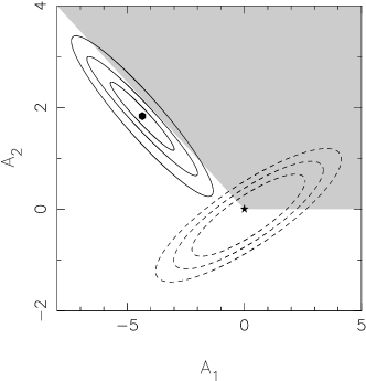
Figure 2: The ($A_{1},A_{2}$) parameter space for the ansatz (7). The light grey shaded area shows the allowed region if dark energy satisfies the weak energy condition both currently and in the past: $w(z)\geq-1,z\geq 0$. The $\chi^{2}$ surface has two minima, a shallow minimum at $A_{1}=0.177,A_{2}=-0.119$ with $\chi^{2}_{\rm shallow}=1.0402$ and a deeper minimum at $A_{1}=-4.360,A_{2}=1.829$ with $\chi^{2}_{\rm deep}=1.0056$. The deeper minimum is marked by a bullet. The solid contours surrounding the deeper minimum are $1\sigma,2\sigma,3\sigma$ contours of constant $\Delta\chi^{2}$ where $\Delta\chi^{2}=\chi^{2}-\chi^{2}_{\rm deep}$. Similarly the dashed contours surrounding the shallower minimum are $1\sigma,2\sigma,3\sigma$ contours of constant $\Delta\chi^{2}$ where $\Delta\chi^{2}=\chi^{2}-\chi^{2}_{\rm shallow}$. Note that the $\Lambda$CDM model (marked by a solid star) corresponds to $A_{1}=A_{2}=0$ which is very close to the shallow minimum.

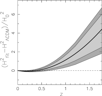
Figure 3: The deviation of $H^{2}/H_{0}^{2}$ from corresponding $\Lambda$CDM values over redshift for the ansatz (7). The thick solid line shows the best-fit, the light grey contour represents the $1\sigma$ confidence level, and the dark grey contour represents the $2\sigma$ confidence level around the best-fit. The dashed horizontal line denotes $\Lambda$CDM. $\Omega_{0{\rm m}}=0.3$ is assumed.

Results :

We first show preliminary results for which the matter density is fixed at a constant value of $\Omega_{0{\rm m}}=0.3$. A detailed look at the $\chi^{2}$ surface in the ($A_{1},A_{2}$) plane (figure 2) reveals the existence of two minima in $\chi^{2}$, a shallower one close to $\Lambda$CDM ($A_{1}=0.177,A_{2}=-0.119,w_{0}=-1.03,\chi^{2}=1.0402$), and a deeper minimum at $A_{1}=-4.360,A_{2}=1.829,w_{0}=-1.33,\chi^{2}=1.0056$. We would like to draw the readers attention to the fact that imposing the prior $w(z)\geq-1\ (z\geq 0)$ amounts to disallowing a significant region of parameter space (the unshaded region in figure 2). Consequently an analysis which assumes $w(z)\geq-1$ loses all information about the region $2\sigma$ around the deeper minimum ! Since we have no reason (observational or theoretical) to favour either minimum over the other, we shall always choose the deeper minimum as our best-fit in all the subsequent calculations.

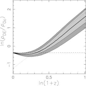
Figure 4: The logarithmic variation of dark energy density $\rho_{\rm DE}/\rho_{0{\rm c}}$ (where $\rho_{0{\rm c}}=3H_{0}^{2}/8\pi G$ is the present day critical density) with redshift for the ansatz (7). The thick solid line shows the best-fit, the light grey contour represents the $1\sigma$ confidence level, and the dark grey contour represents the $2\sigma$ confidence level around the best-fit. The dashed horizontal line denotes $\Lambda$CDM and the dotted line represents matter density $\Omega_{0{\rm m}}(1+z)^{3}$, $\Omega_{0{\rm m}}=0.3$ is assumed.

In the figure 3, we plot the deviation of the squared Hubble parameter $H^{2}/H_{0}^{2}$ from $\Lambda$CDM over redshift for the best-fit. We note that the quantity $H^{2}/H_{0}^{2}$ has a simple linear relationship with the parameters of the fit (Eq 7), therefore the errors in this quantity increase with redshift. Another quantity of interest is the energy density of dark energy. For this ansatz, $\tilde{\rho}_{\rm DE}=\rho_{\rm DE}/\rho_{0{\rm c}}=A_{0}+A_{1}x+A_{2}x^{2}$ (where $\rho_{0{\rm c}}=3H_{0}^{2}/8\pi G$ is the present day critical density). The figure 4 shows the logarithmic variation of $\tilde{\rho}_{\rm DE}$ with redshift. In this figure too the errors increase with redshift. An interesting point to note is that initially, dark energy density decreases with redshift, showing the phantom-like nature ($w<-1$) of dark energy at lower redshifts of $z\lower 3.87495pt\hbox{ $\buildrel<\over{\sim}$}~{}0.25$, while at higher redshifts, the dark energy density begins to track the matter density. Before moving on to the second derivative of the luminosity distance (e.g., the equation of state) we may obtain more information from the dark energy density by considering a weighted average of the equation of state :

$$1+\bar{w}=\frac{1}{\Delta\ {\rm ln}(1+z)}\int(1+w(z))\frac{dz}{1+z}\,\,,$$ (16)

where $\Delta$ denotes the total change of the variable between integration limits. This quantity can be elegantly expressed in terms of the difference in energy densities over a range of redshift as

$$1+\bar{w}=\frac{1}{3}\frac{\Delta\ {\rm ln}\tilde{\rho}_{\rm DE}}{\Delta\ {\rm ln}(1+z)}\,\,.$$ (17)

Thus the variation in the dark energy density depicted in figure 4 is very simply related to the weighted average equation of state !

Table 1: The weighted average $\bar{w}$ (eq 16) over specified redshift ranges. The best-fit value and $1\sigma$ and $2\sigma$ deviations from the best-fit are shown.

$\Delta z$	$\bar{w}$	$1\sigma$	$2\sigma$
$0-0.414$	$-0.969$	${}^{+0.120}_{-0.089}$	${}^{+0.198}_{-0.199}$
$0.414-1$	$-0.108$	${}^{+0.230}_{-0.240}$	${}^{+0.242}_{-0.360}$
$1-1.756$	$0.069$	${}^{+0.100}_{-0.080}$	${}^{+0.130}_{-0.180}$

$\Omega_{0{\rm m}}=0.2$                                                $\Omega_{0{\rm m}}=0.3$                                                $\Omega_{0{\rm m}}=0.4$

$\begin{array}[]{@{\hspace{-0.4in}}c@{\hspace{0.3in}}c@{\hspace{0.3in}}c}\lx@intercol\mbox{}\hfil\lx@intercol&\lx@intercol\mbox{}\hfil\lx@intercol&\lx@intercol\mbox{}\hfil\lx@intercol\\[-14.22636pt] \epsfbox{h_exp_w_mi_tot.epsi}\hfil\hskip 21.68121pt&\epsfbox{h_exp_w_tot.epsi}\hfil\hskip 21.68121pt&\epsfbox{h_exp_w_pl_tot.epsi}\\ \mbox{\bf(a)}\hfil\hskip 21.68121pt&\mbox{\bf(b)}\hfil\hskip 21.68121pt&\mbox{\bf(c)}\end{array}$

Figure 5: The evolution of $w(z)$ with redshift for different values of $\Omega_{0{\rm m}}$. The reconstruction is done using the polynomial fit to dark energy, equation (7). In each panel, the thick solid line shows the best-fit, the light grey contour represents the $1\sigma$ confidence level, and the dark grey contour represents the $2\sigma$ confidence level around the best-fit. The dashed line represents $\Lambda$CDM. No priors are assumed on $w(z)$. The $\chi^{2}$ per degree of freedom for each case is given in Table 2.

Table 2: $\chi^{2}$ per degree of freedom for best-fit and $\Lambda$CDM models. $w_{0}$ is the present value of the equation of state of dark energy in best-fit models. $\chi^{2}_{\rm Pr}$ refers to the best fit after imposition of the WEC prior $w(z)\geq-1\ (z\geq 0)$.

	Best-fit		Confidence levels		$w(z)\geq-1$	$\Lambda$CDM
$\Omega_{0{\rm m}}$	$w_{0}$	$\chi^{2}_{\rm min}$	$\chi^{2}_{1\sigma}$	$\chi^{2}_{2\sigma}$	$\chi^{2}_{\rm Pr}$	$\chi^{2}$
$0.10$	$-1.093$	$1.0077$	$1.0213$	$1.0442$	$1.0359$	$1.1242$
$0.20$	$-1.198$	$1.0071$	$1.0207$	$1.0436$	$1.0384$	$1.0663$
$0.30$	$-1.334$	$1.0056$	$1.0192$	$1.0421$	$1.0409$	$1.0417$
$0.40$	$-1.470$	$1.0043$	$1.0179$	$1.0408$	$1.0578$	$1.0638$
$0.50$	$-1.606$	$1.0038$	$1.0174$	$1.0403$	$1.0912$	$1.1168$

In table 1 we show the values of $\bar{w}$ obtained using different ranges in redshift for our best-fit with corresponding $1\sigma$ and $2\sigma$ errors. We have taken the ranges of integration to be approximately equally spaced in ln$(1+z)$, with the upper limit set by the furthest supernova known at present. The values of $\bar{w}$ may be calculated using the equation (16) (which uses the second derivative of the luminosity distance), or they can simply be read off from figure 4 using equation (17). From this table, a “metamorphosis” in the properties of dark energy occurring somewhere between $z\sim 0$ and $z\sim 1$ can be clearly seen (note that, effectively, one needs to differentiate $d_{L}(z)$ only once to come to this conclusion).

$\Omega_{0{\rm m}}=0.2$                                                $\Omega_{0{\rm m}}=0.3$                                                $\Omega_{0{\rm m}}=0.4$

$\begin{array}[]{@{\hspace{-0.4in}}c@{\hspace{0.3in}}c@{\hspace{0.3in}}c}\lx@intercol\mbox{}\hfil\lx@intercol&\lx@intercol\mbox{}\hfil\lx@intercol&\lx@intercol\mbox{}\hfil\lx@intercol\\[-14.22636pt] \epsfbox{h_exp_w_mi_cons.epsi}\hfil\hskip 21.68121pt&\epsfbox{h_exp_w_cons.epsi}\hfil\hskip 21.68121pt&\epsfbox{h_exp_w_pl_cons.epsi}\\ \mbox{\bf(a)}\hfil\hskip 21.68121pt&\mbox{\bf(b)}\hfil\hskip 21.68121pt&\mbox{\bf(c)}\end{array}$

Figure 6: The evolution of $w(z)$ with redshift for different values of $\Omega_{0{\rm m}}$, using the prior $w(z)\geq-1,z\geq 0$. The reconstruction is done using the polynomial fit to dark energy, equation (7). In each panel, the thick solid line shows the best-fit, the light grey contour represents the $1\sigma$ confidence level, and the dark grey contour represents the $2\sigma$ confidence level around the best-fit. The hatched region is forbidden by the prior $w(z)\geq-1$. The dashed line represents $\Lambda$CDM. The $\chi^{2}$ per degree of freedom for each case is given in Table 2.

$\begin{array}[]{c@{\hspace{0.4in}}c}\lx@intercol\mbox{}\hfil\lx@intercol&\lx@intercol\mbox{}\hfil\lx@intercol\\[0.0pt] \epsfbox{h_exp_w_m.epsi}\hfil\hskip 28.90755pt&\epsfbox{h_exp_w_m_cons.epsi}\\ \mbox{\bf(a)}\hfil\hskip 28.90755pt&\mbox{\bf(b)}\end{array}$

Figure 7: Evolution of $w(z)$ with redshift using the 2dF prior $\Omega_{0{\rm m}}h=0.2\pm 0.03$, with (a) no priors on $w(z)$, and (b) the prior $w(z)\geq-1,~{}z\geq 0$. The reconstruction is done using the polynomial fit to dark energy, equation (7). In both panels, the thick solid line represents the best-fit, the dashed line represents $\Lambda$CDM, the light grey contour represents $1\sigma$ confidence level, and the dark grey contour represents the $2\sigma$ confidence level. In the right hand panel, the hatched region is forbidden by the prior $w(z)\geq-1$.

We now reconstruct the equation of state of dark energy which, for the ansatz (7), has the form

$$w(z)=-1+\frac{x}{3}\frac{A_{1}+2A_{2}x}{A_{0}+A_{1}x+A_{2}x^{2}},~{}~{}x=1+z~{}.$$ (18)

(Note that, since $w(z)$ was derived from the ansatz (7), its domain of validity is $z\lower 3.87495pt\hbox{ $\buildrel<\over{\sim}$}~{}{\rm few}$.) In figures 5 (a), (b), (c), we show the evolution of the equation of state $w(z)$ with redshift for different values of $\Omega_{0{\rm m}}$. The $1\sigma$ and $2\sigma$ limits are shown in each case. The $\chi^{2}$ per degree of freedom for the best-fit for the different cases is given in Table 2. We find that for $0.2<\Omega_{0{\rm m}}<0.4$, the behaviour of the equation of state does not change significantly with change in the matter density. However, for larger values of $\Omega_{0{\rm m}}$, a smaller current value of $w_{0}=w(z=0)$ is preferred. In all three cases considered, the present value of the equation of state is $w_{0}\lower 3.87495pt\hbox{ $\buildrel<\over{\sim}$}~{}-1.2$ for the best-fit, and the equation of state rises steeply from $w\lower 3.87495pt\hbox{ $\buildrel<\over{\sim}$}~{}-1.2$ to $w\simeq 0$ with redshift. In fact, the behaviour of $w$ appears to be extremely different from that in $\Lambda$CDM ($w=-1$). We note here that, for this analysis, the errors on $w$ appear to decrease with redshift. This may appear counter-intuitive, since there are fewer SNe at higher redshifts, but this is merely a construct of the fact that $w$ depends non-linearly on the parameters of the ansatz (see appendix A).

Quintessence models satisfy the weak energy condition (WEC) $\rho+p={\dot{\phi}}^{2}\geq 0$ and it would be interesting to see how the imposition of the WEC as a prior on the equation of state will affect the results of our analysis. We therefore perform the same analysis as above with the added constraint $w_{0}\geq-1$ (note that this implies $w(z)\geq-1$ for all $z\geq 0$ for our fitting function of $H(z)$ provided $A_{2}\geq 0$). The results are shown in the figures 6 (a), (b), (c). We see that in this case the errors are larger and the evolution of the equation of state with redshift follows a much gentler slope. Such an equation of state would be largely consistent with the cosmological constant model. (These results are in broad agreement with an earlier analysis of Saini et al.  (2000) in which a smaller SNe data set was used and a different ansatz for the luminosity distance was applied.)

In Table 2, we show how the $\chi^{2}$ for the best-fit evolving dark energy models compare with that for $\Lambda$CDM. We find that $\chi^{2}_{\Lambda{\rm CDM}}>\chi^{2}_{\rm best-fit}$ always. For $\Omega_{0{\rm m}}=0.3$, the value of $\chi^{2}_{\Lambda{\rm CDM}}$ is just within $2\sigma$ of the best fit $\chi^{2}$, but for $\Omega_{0{\rm m}}=0.2$, or $\Omega_{0{\rm m}}=0.4$, $\chi^{2}_{\Lambda{\rm CDM}}$ is outside the $2\sigma$ limits of the best-fit. It is also noteworthy that when the prior $w(z)\geq-1\ (z\geq 0)$ is used, the best-fit model has a slowly evolving equation of state with $w_{0}=-1$ and the $\chi^{2}$ for the best-fit becomes smaller for a smaller value of the matter density. When no priors are assumed on $w$, the trend reverses, and better fits are obtained for larger values of $\Omega_{0{\rm m}}$. From this it appears that at least at $1\sigma$ the evolving dark energy model is favoured over $\Lambda$CDM, and it does as well, if not better at the $2\sigma$ level, depending upon the value of the present-day matter density.

Using Priors on $\Omega_{0{\rm m}}$ :

Instead of assuming an exact value for $\Omega_{0{\rm m}}$, which is somewhat optimistic given the present observational scenario, we may use the 2dF prior on $\Omega_{0{\rm m}}$ and calculate $w(z)$ as a function of $(\Omega_{0{\rm m}},A_{1},A_{2})$. It should be noted here that the 2dF error bars on $\Omega_{0{\rm m}}h$ have been calculated using 2dF data in conjunction with CMB, and this calculation assumes a $\Lambda$CDM model, therefore this prior should be used more as a benchmark for the value of $\Omega_{0{\rm m}}$ rather than as an absolute when considering evolving dark energy models. The resultant “marginalised” $w$ is shown as a function of the redshift in figure 7 (a). The nature of the equation of state for the analysis with the added prior $w(z)\geq-1\ (z\geq 0)$ is shown in figure 7 (b). We find that the general nature of evolution of the equation of state is not changed by adding this extra information on the matter density. If no priors are assumed on the equation of state to begin with, $w(z)$ still rises sharply from $w_{0}\lower 3.87495pt\hbox{ $\buildrel<\over{\sim}$}~{}-1$ up to $w\simeq 0$ at maximum redshift and the analysis appears to favour a fast-evolving equation of state of dark energy over the standard $\Lambda$CDM model. If a prior $w\geq-1$ is assumed, then the marginalised equation of state is more consistent with the cosmological constant. From this we see that marginalisation over $\Omega_{0{\rm m}}$ does not lead to any significant change in our results. In the subsequent sections, we will show our results for $\Omega_{0{\rm m}}=0.3$.

From the above analysis, we find, therefore, that our results change significantly depending upon whether or not the prior $w\geq-1$ is imposed. We saw earlier that in the absence of any prior on $w(z)$, the best-fit equation of state rose from $w\lower 3.87495pt\hbox{ $\buildrel<\over{\sim}$}~{}-1$ at $z=0$ to $w\simeq 0$ at $z\sim 1$. By imposing a prior on the equation of state, we effectively screen off a sizeable part of the parameter space (see figure 2), and therefore the reconstruction is forced to choose its best-fit away from the true minima of the $\chi^{2}$ surface. The effect of imposing a prior on $w(z)$ is therefore to make the best-fit $w(z)$ grow much more slowly with $w=-1$ being preferred at $z=0$. Our results show that the reconstructed equation of state with the prior $w\geq-1$ is in good agreement with a cosmological constant at the $68\%$ CL. However, if no prior is imposed, then the steeply evolving dark energy models are favoured over the cosmological constant at $1\sigma$, and are at least as likely as the cosmological constant at the $2\sigma$ level.

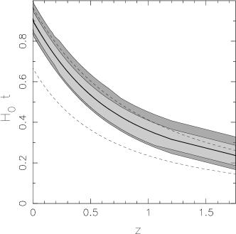
Figure 8: The age of the universe, $H_{0}t(z)$, is shown as a function of the redshift for $\Omega_{0{\rm m}}=0.3$. The reconstruction is done using the polynomial fit to dark energy, equation (7). The thick solid line represents the best-fit, the light grey contour represents $1\sigma$ confidence level, and the dark grey contour represents the $2\sigma$ confidence level. The upper (lower) dashed line represents $\Lambda$CDM (SCDM).

Age and Deceleration Parameter of the Universe:

We may also use this ansatz to calculate other quantities of interest, such as the age of the universe, $t(z)$, and the deceleration parameter, $q(z)$:

$$t(z) = \int_{1+z}^{\infty}\frac{dx}{xH(x)}$$ (19)

$$q(z) = -\frac{\ddot{a}}{aH^{2}}\equiv\frac{H^{\prime}}{H}x-1\,\,.$$ (20)

where $x=1+z$.

In figure 8 we plot the evolution of the age of the universe with redshift. We find that the best-fit age of the universe today is $t_{0}=12.8$ Gyrs if the Hubble parameter is taken to be $H_{0}=72\ {\rm km\ s^{-1}\ Mpc^{-1}}$, which is slightly lower than the age of a $\Lambda$CDM universe, $t_{0}=13.4$ Gyrs (both values are for $\Omega_{0{\rm m}}=0.3$). At the $2\sigma$ level, the age of the universe today would vary between $11.2\leq t_{0}\leq 13.6$ Gyrs.

Figure 10 shows the evolution of the deceleration parameter with redshift. We find that the behaviour of the deceleration parameter for the best-fit universe is quite different from that in $\Lambda$CDM cosmology. Thus, the current value of $q_{0}\simeq-0.9$ is significantly lower than $q_{0}\simeq-0.55$ for $\Lambda$CDM (assuming $\Omega_{0{\rm m}}=0.3$). Furthermore the rise of $q(z)$ with redshift is much steeper in the case of the best-fit model, with the result that the universe begins to accelerate at a comparatively lower redshift $z\simeq 0.3$ (compared with $z\simeq 0.7$ for $\Lambda$CDM) and the matter dominated regime ($q\simeq 1/2$) is reached by $z\sim 1$.

$H_{0}=72\pm 8\ {\rm km\ s^{-1}\ Mpc^{-1}}$

$\begin{array}[]{@{\hspace{-0.4in}}c@{\hspace{0.3in}}c@{\hspace{0.3in}}c}\lx@intercol\mbox{}\hfil\lx@intercol&\lx@intercol\mbox{}\hfil\lx@intercol&\lx@intercol\mbox{}\hfil\lx@intercol\\[-14.22636pt] \epsfbox{h_exp_w_age1.epsi}\hfil\hskip 21.68121pt&\epsfbox{h_exp_w_age.epsi}\hfil\hskip 21.68121pt&\epsfbox{h_exp_w_age2.epsi}\\ \mbox{\bf(a)}\hfil\hskip 21.68121pt&\mbox{\bf(b)}\hfil\hskip 21.68121pt&\mbox{\bf(c)}\end{array}$

$H_{0}=66\pm 6\ {\rm km\ s^{-1}\ Mpc^{-1}}$

$\begin{array}[]{@{\hspace{-0.4in}}c@{\hspace{0.3in}}c@{\hspace{0.3in}}c}\lx@intercol\mbox{}\hfil\lx@intercol&\lx@intercol\mbox{}\hfil\lx@intercol&\lx@intercol\mbox{}\hfil\lx@intercol\\[-14.22636pt] \epsfbox{h_exp_w_age4.epsi}\hfil\hskip 21.68121pt&\epsfbox{h_exp_w_age3.epsi}\hfil\hskip 21.68121pt&\epsfbox{h_exp_w_age5.epsi}\\ \mbox{\bf(d)}\hfil\hskip 21.68121pt&\mbox{\bf(e)}\hfil\hskip 21.68121pt&\mbox{\bf(f)}\end{array}$

Figure 9: The evolution of $w(z)$ with redshift for $\Omega_{0{\rm m}}=0.3$ using a Gaussian prior on the age of the universe today: $t_{0}=13\pm 1$Gyrs (figures (a) and (d)), $t_{0}=14\pm 1$Gyrs (figures (b) and (e)), and $t_{0}=15\pm 1$Gyrs (figures (c) and (f)). The reconstruction is done using the polynomial fit to dark energy, equation (7). The top panel is obtained using a Gaussian prior $H_{0}=72\pm 8\ {\rm km\ s^{-1}\ Mpc^{-1}}$, while for the bottom panel, $H_{0}=66\pm 6\ {\rm km\ s^{-1}\ Mpc^{-1}}$. No priors are assumed on $w(z)$. In each panel, the thick solid line shows the best-fit, the light grey contour represents the $1\sigma$ confidence level, and the dark grey contour represents the $2\sigma$ confidence level around the best-fit. The dashed line represents $\Lambda$CDM. The $\chi^{2}$ per degree of freedom for each case is given in Table 3.

Table 3: $\chi^{2}$ per degree of freedom for the ansatz (7) which best fits the SNe data after different age priors are imposed. $w_{0}$ is the present value of the equation of state of dark energy in best-fit models.

$H_{0}$	$t_{0}$	Best-fit
${\rm km\ s^{-1}\ Mpc^{-1}}$	${\rm Gyrs}$	$w_{0}$	$\chi^{2}_{\rm min}$
$72\pm 8$	$13\pm 1$	$-1.271$	$1.0062$
	$14\pm 1$	$-1.099$	$1.0197$
	$15\pm 1$	$-0.904$	$1.0407$
$66\pm 6$	$13\pm 1$	$-1.553$	$1.0139$
	$14\pm 1$	$-1.324$	$1.0057$
	$15\pm 1$	$-1.153$	$1.0146$

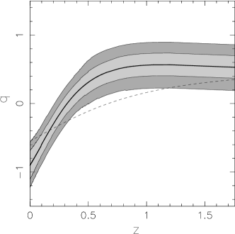
Figure 10: Evolution of deceleration parameter of the universe, $q(z)$ with redshift for $\Omega_{0{\rm m}}=0.3$. The reconstruction is done using the polynomial fit to dark energy, equation (7). The thick solid line represents the best-fit, the light grey contour represents $1\sigma$ confidence level, and the dark grey contour represents the $2\sigma$ confidence level. The dashed line represents $\Lambda$CDM.

Using Priors on Age of the Universe :

Important consistency checks on our best-fit Universe may be provided by observations of the age of the Universe. Unfortunately, estimates of the age of the universe from different methods can produce widely varying results one reason for which is that estimates of the Hubble parameter itself can vary significantly. For instance, the HST key project yields $H_{0}=72\pm 8\ {\rm km\ s^{-1}\ Mpc^{-1}}$, while studies of the Sunyaev-Zeldovich effect in galaxy clusters give a significantly lower value $H_{0}=60\pm 10\ {\rm km\ s^{-1}\ Mpc^{-1}}$ (Krauss, 2001). Estimates of the ages of the oldest globular clusters suggest $t_{0}=12.5\pm 2.5$ Gyrs, at the $95\%$ confidence level (Krauss, 2001; Krauss & Chaboyer, 2001; Gnedin, Lahav & Rees, 2001; Hansen et al. , 2002; Gratton et al. , 2003; Marchi et al. , 2003) and this age estimate is consistent with several other measurements including observations of eclipsing spectroscopic binaries (Thompson et al. , 2001; Chaboyer & Krauss, 2002), results from radioactive dating of a metal-poor star (Cayrel et al. , 2001) and WMAP data (Spergel et al. , 2003) (see also Alcaniz, Jain and Dev (2002)). The results from the WMAP experiment suggest $t_{0}=13.4\pm 0.3$ Gyrs with a Hubble parameter $H_{0}=72\pm 5\ {\rm km\ s^{-1}\ Mpc^{-1}}$, for $\Lambda$CDM cosmology (which satisfies the WEC). Adding SDSS and SNe Ia data to WMAP, Tegmark et al.  (2003) find an age of $t_{0}=14.1^{1.0}_{0.9}$ Gyrs for a slightly closed $\Lambda$CDM universe with $H_{0}=66^{6.7}_{6.4}\ {\rm km\ s^{-1}\ Mpc^{-1}}$. Although these results cannot be carried over to evolving dark energy models including those implied by our best-fit reconstruction (which violate the WEC) they provide an indication of the range within which the age of the universe might vary. Keeping in mind these various results, we use two different priors on the Hubble parameter: $H_{0}=72\pm 8\ {\rm km\ s^{-1}\ Mpc^{-1}}$ ($1\sigma$ bound from HST; Freedman et al.  (2001)), and $H_{0}=66\pm 6\ {\rm km\ s^{-1}\ Mpc^{-1}}$ (approximate bound from WMAP, SDSS, SNe Ia; Tegmark et al.  (2003)). For each case, we choose three different Gaussian priors on the present age of the universe: $t_{0}=13\pm 1\ {\rm Gyrs},\ 14\pm 1\ {\rm Gyrs},\ {\rm and}\ 15\pm 1\ {\rm Gyrs}$ respectively, and perform the reconstruction for a $\Omega_{0{\rm m}}=0.3$ universe. The results are shown in the figure 9. We find that, for a Hubble parameter of $H_{0}=72\pm 8\ {\rm km\ s^{-1}\ Mpc^{-1}}$, and with an additional prior on the age of the universe $t_{0}=13\pm 1$ Gyrs, the best-fit remains nearly the same, showing a rapid evolution of the equation of state from $w\sim 0$ at $z\sim 1$ to $w\sim-1.2$ at $z=0$, and the errors become narrower. As the age is increased, the best-fit equation of state evolves more slowly, and the $\chi^{2}_{\rm dof}$ also increases (see Table 3). For the prior $H_{0}=66\pm 6\ {\rm km\ s^{-1}\ Mpc^{-1}}$, we find that the lowest $\chi^{2}_{\rm dof}$ is obtained for the age prior of $t_{0}=14\pm 1$ Gyrs, which once again matches our best-fit. It should be noted that the errors are smaller in all cases, even though the $\chi^{2}$ may be larger. We must remember that the addition of a new prior which is consistent with the underlying dataset would lead to a natural reduction in errors. However, the addition of a prior inconsistent with the dataset would lead to a shift of the likelihood maximum as well as a reduction in errors, and the results would then fail to reflect the actual information present in the dataset. That this is happening here for the higher values of age can be seen from the fact that although the errors are reduced, the $\chi^{2}_{\rm dof}$ is actually larger. Therefore priors from other observations should be added prudently to ensure that they do not lead to incorrect representation of the data. Since there is as yet no clear model independent consensus on the age of the universe, the results we obtain in this section should be interpreted with a degree of caution.

Figure 10 shows the evolution of the deceleration parameter with redshift. We find that the behaviour of the deceleration parameter for the best-fit universe is quite different from that in $\Lambda$CDM cosmology. Thus, the current value of $q_{0}\simeq-0.9$ is significantly lower than $q_{0}\simeq-0.55$ for $\Lambda$CDM (assuming $\Omega_{0{\rm m}}=0.3$). Furthermore the rise of $q(z)$ with redshift is much steeper in the case of the best-fit model, with the result that the universe begins to accelerate at a comparatively lower redshift $z\simeq 0.3$ (compared with $z\simeq 0.7$ for $\Lambda$CDM) and the matter dominated regime ($q\simeq 1/2$) is reached by $z\sim 1$.

$\begin{array}[]{c@{\hspace{0.4in}}c}\lx@intercol\mbox{}\hfil\lx@intercol&\lx@intercol\mbox{}\hfil\lx@intercol\\[0.0pt] \epsfbox{h_exp_dens_hzt.epsi}\hfil\hskip 28.90755pt&\epsfbox{h_exp_dens_scp.epsi}\\ \mbox{\bf(a)}\hfil\hskip 28.90755pt&\mbox{\bf(b)}\end{array}$

Figure 11: The logarithmic variation of dark energy density $\rho_{\rm DE}(z)/\rho_{0{\rm c}}$ (where $\rho_{0{\rm c}}=3H_{0}^{2}/8\pi G$ is the present day critical density) with redshift for $\Omega_{0{\rm m}}=0.3$, using (a) HZT data, and (b) SCP data. The reconstruction is done using the polynomial fit to dark energy, equation (7). No priors are assumed on $w(z)$. In both panels, the thick solid line shows the best-fit, the light grey contour represents the $1\sigma$ confidence level, and the dark grey contour represents the $2\sigma$ confidence level around the best-fit. The horizontal dashed line represents $\Lambda$CDM, and the dotted line represents matter density.

$\begin{array}[]{c@{\hspace{0.4in}}c}\lx@intercol\mbox{}\hfil\lx@intercol&\lx@intercol\mbox{}\hfil\lx@intercol\\[0.0pt] \epsfbox{h_exp_w_hzt.epsi}\hfil\hskip 28.90755pt&\epsfbox{h_exp_w_scp.epsi}\\ \mbox{\bf(a)}\hfil\hskip 28.90755pt&\mbox{\bf(b)}\end{array}$

Figure 12: The evolution of $w(z)$ with redshift for $\Omega_{0{\rm m}}=0.3$, using (a) HZT data, and (b) SCP data. The reconstruction is done using the polynomial fit to dark energy, equation (7). No priors are assumed on $w(z)$. In both panels, the thick solid line shows the best-fit, the light grey contour represents the $1\sigma$ confidence level, and the dark grey contour represents the $2\sigma$ confidence level around the best-fit. The horizontal dashed line represents $\Lambda$CDM.

$\begin{array}[]{c@{\hspace{0.4in}}c}\lx@intercol\mbox{}\hfil\lx@intercol&\lx@intercol\mbox{}\hfil\lx@intercol\\[0.0pt] \epsfbox{h_exp_w_hzt_cons.epsi}\hfil\hskip 28.90755pt&\epsfbox{h_exp_w_scp_cons.epsi}\\ \mbox{\bf(a)}\hfil\hskip 28.90755pt&\mbox{\bf(b)}\end{array}$

Figure 13: The evolution of $w(z)$ with redshift for $\Omega_{0{\rm m}}=0.3$, with the prior $w(z)\geq-1,~{}z\geq 0$, using (a) HZT data, and (b) SCP data. The reconstruction is done using the polynomial fit to dark energy, equation (7). In both panels, the thick solid line shows the best-fit, the light grey contour represents the $1\sigma$ confidence level, and the dark grey contour represents the $2\sigma$ confidence level around the best-fit. The hatched region is forbidden by the prior $w(z)\geq-1$. The horizontal dashed line represents $\Lambda$CDM.

2.2 Robustness of Results :

Based on the above analysis, it is tempting to conclude that the dominant component of the universe today is dark energy with a steeply evolving equation of state which marginally violates the weak energy condition. (Of course, the less radical possibility of weakly time dependent dark energy satisfying the weak energy condition remains an alternative, too.) However, before any such dramatic claims are made, we need to check if our results are in any fashion a consequence of inherent bias in the statistical analysis itself, or in the sampling of the data. We therefore perform the following simple exercises to satisfy ourselves of the robustness of our results.

Using Different Subsets of Supernova Data :

In an attempt to understand how the nature of the reconstructed equation of state is dependent on the distribution of data, we perform the reconstruction exercise on different samples of data. We have confined ourselves to the case where $\Omega_{0{\rm m}}=0.3$ for these exercises. Firstly, we may exclude the SCP data points from the 172 SNe primary fit, leading to a subsample of 130 SNe. We call this the HZT sample. Figures 11(a) and 12(a) show the result of performing the analysis on this subsample without any constraints. The $\chi^{2}$ per degree of freedom for the best-fit is $\chi^{2}_{\rm HZT}=0.9707$, which is lower than $\chi^{2}_{\Lambda{\rm CDM}}=0.9939$ for this sample. In this case we find that, though the error bars are slightly larger, overall the dark energy density behaves in the same way as before (compare figure 11(a) with figure 4), showing phantom like ($w<-1$) behaviour at lower redshifts and tracking matter at higher redshifts. The equation of state of dark energy also evolves much in the same way as when the entire sample is used (compare figure 12(a) with figure 5(b)), starting at $w_{0}\lower 3.87495pt\hbox{ $\buildrel<\over{\sim}$}~{}-1$ and evolving rapidly to $w\simeq 0$. We may also use a sample complementary to this sample, where all the SCP data points published till date are considered, along with the low redshift Calan-Tololo sample. This leads to a sample of 58 SNe (Perlmutter et al. , 1999; Knop et al. , 2003), which we call the SCP sample. Using this sample, we obtain the figures 11(b) and 12(b). The best-fit has a chi-squared per degree of freedom: $\chi^{2}_{\rm SCP}=1.0147$, lower than $\chi^{2}_{\Lambda{\rm CDM}}=1.0369$ for this sample. We find that here too, the dark energy density initially decreases and then starts tracking matter. The equation of state shows signs of rising steeply at low redshifts, but since the highest redshift in this sample is $z=0.86$, the behaviour of $w$ beyond this redshift cannot be predicted, therefore the apparent flattening out of the curve beyond a redshift of one cannot be seen in this case. For both these subsets of data, we may repeat the exercise using the prior $w(z)\geq-1\ (z\geq 0)$. The results obtained for the equation of state, as seen in figures 13(a), (b), are once again commensurate with the results obtained earlier for the full sample (figure 6(b)). We may therefore conclude from this exercise that subsampling the data does not significantly affect our results, and the steep evolution of the equation of state of dark energy is not a construct of the uneven sampling of the supernovae, but rather, reflects the actual nature of dark energy.

Testing our Ansatz against fiducial dark energy models :

$w=-0.5$                                                ${\rm Chaplygin\ Gas}$                                                $w=-1.2+z$

$\begin{array}[]{@{\hspace{-0.4in}}c@{\hspace{0.3in}}c@{\hspace{0.3in}}c}\lx@intercol\mbox{}\hfil\lx@intercol&\lx@intercol\mbox{}\hfil\lx@intercol&\lx@intercol\mbox{}\hfil\lx@intercol\\[-14.22636pt] \epsfbox{h_exp_w_sim_w.epsi}\hfil\hskip 21.68121pt&\epsfbox{h_exp_w_sim_cg.epsi}\hfil\hskip 21.68121pt&\epsfbox{h_exp_w_sim_ev.epsi}\\ \mbox{\bf(a)}\hfil\hskip 21.68121pt&\mbox{\bf(b)}\hfil\hskip 21.68121pt&\mbox{\bf(c)}\end{array}$

Figure 14: Reconstructed equation of state, $w(z)$, for simulated data corresponding to three fiducial dark energy models: (a) quiessence with $w=-0.5$, (b) generalised Chaplygin gas: $p=A/\rho^{\alpha}$, with $\alpha=0.5,w_{0}=-0.9$, and (c) $w=w_{0}+w_{1}z$ with $w_{0}=-1.2,w_{1}=1.0$. $\Omega_{0{\rm m}}=0.3$ is assumed and the reconstruction is done using the polynomial fit to dark energy, equation (7). In each panel, the thick solid line is the best-fit, the dashed line represents the exact model value, and the light grey contour represents the $1\sigma$ confidence level around the best fit.

$\begin{array}[]{c@{\hspace{0.4in}}c}\lx@intercol\mbox{}\hfil\lx@intercol&\lx@intercol\mbox{}\hfil\lx@intercol\\[0.0pt] \epsfbox{lin_w.epsi}\hfil\hskip 28.90755pt&\epsfbox{lin_w_cons.epsi}\\ \mbox{\bf(a)}\hfil\hskip 28.90755pt&\mbox{\bf(b)}\end{array}$

Figure 15: Evolution of $w(z)$ with redshift for $\Omega_{0{\rm m}}=0.3$ with (a) no priors on $w(z)$, and (b) the prior $w(z)\geq-1\ (z\geq 0)$. The reconstruction is done using Linder’s fit to the equation of state, equation 22. In both panels, the thick solid line represents the best-fit, the dashed line represents $\Lambda$CDM, and the light grey contour represents the $1\sigma$ confidence level. In the right hand panel, the hatched region is forbidden by the prior $w(z)\geq-1$.

$\begin{array}[]{c@{\hspace{0.4in}}c}\lx@intercol\mbox{}\hfil\lx@intercol&\lx@intercol\mbox{}\hfil\lx@intercol\\[0.0pt] \epsfbox{bass_w.epsi}\hfil\hskip 28.90755pt&\epsfbox{bass_w_cons.epsi}\\ \mbox{\bf(a)}\hfil\hskip 28.90755pt&\mbox{\bf(b)}\end{array}$

Figure 16: Evolution of $w(z)$ with redshift for $\Omega_{0{\rm m}}=0.3$ with (a) no priors on $w(z)$, and (b) the prior $w(z)\geq-1\ (z\geq 0)$. The reconstruction is done using a four-parameter fit to the equation of state, equation 24. In both panels, the thick solid line represents the best-fit, the dashed line represents $\Lambda$CDM, and the light grey contour represents the $1\sigma$ confidence level. In the right hand panel, the hatched region is forbidden by the prior $w(z)\geq-1$.

The crucial question of course is whether the reconstructed equation of state of dark energy depends upon the ansatz which is used in the exercise, i.e. , whether the behaviour of the equation of state merely reflects a bias in the ansatz itself. In this section we show how the ansatz performs in recovering dark energy models whose equation of state is known, from simulated data. This ansatz was demonstrated to work extremely well when simulations of SNAP data were used (Alam et al. , 2003). However, simulation of SNAP-like data is an optimistic exercise, since data of this quality is unlikely to be available in the near future. We now demonstrate the accuracy with which the ansatz can recover the fiducial background cosmological model if data is simulated using present-day observational standards. In figures 14 (a), (b), (c), we show how well the ansatz recovers the equation of state for three fiducial models (assuming $\Omega_{0{\rm m}}=0.3$):

(a) a quiessence dark energy model with a constant equation of state: $w=-0.5$,

(b) a generalised Chaplygin gas model with $p=A/\rho^{\alpha}$: with $\alpha=0.5$ and the present-day equation of state $w_{0}=-0.9$, which would give rise to an effective equation of state

$$w(z)=-\frac{|w_{0}|}{|w_{0}|+(1-|w_{0}|)(1+z)^{3(1+\alpha)}}\,,$$ (21)

and

(c) a model with a linearly evolving equation of state: $w(z)=w_{0}+w_{1}z$, with $w_{0}=-1.2,w_{1}=1$.

(For DE models with $w=-1,-2/3,-1/3$ the ansatz is exact therefore we don’t show the results for these cases.)

We find that in all three cases, the fiducial model lies within the $68\%$ confidence limits around the best-fit $w(z)$. Based on this result, we claim that within the $1\sigma$ error bars, the reconstructed equation of state represents the true properties of dark energy when we use real data.

Using other Ansatz :

It is also important to check whether the results of our reconstruction can be replicated using other ansatz such as fits to the luminosity distance or the equation of state. Many different fits have been suggested in the literature (see for example Huterer & Turner (1999), Saini et al.  (2000), Weller & Albrecht (2002), Gerke & Efstathiou (2002)). Here we choose the fit suggested in Linder (2003) in which the equation of state of dark energy is expanded as

$$w(z)=w_{0}+\frac{w_{1}z}{1+z}~{}.$$ (22)

The luminosity distance can therefore be expressed as

$$\frac{d_{L}(z)}{1+z}=\frac{c}{H_{0}}\int_{1}^{1+z}\frac{dx}{\sqrt{\Omega_{0{\rm m}}x^{3}+\Omega_{X}}}\,,\\$$ (23)

where $\Omega_{X}=(1-\Omega_{0{\rm m}})x^{3(1+w_{0}+w_{1})}{\rm exp}[3w_{1}(\frac{1}{x}-1)]$.

We find that for this fit, the errors in the equation of state get larger with redshift, however this fit too demonstrates that the equation of state of dark energy increases rapidly with redshift (figure 15(a)) when no priors are assumed on the equation of state (EOS). The $\chi^{2}$ per degree of freedom at the best-fit is $\chi^{2}_{\rm dof}=1.0298$. When the prior $w(z)\geq-1\ (z\geq 0)$ is invoked, the best-fit EOS remains very close to the $\Lambda$CDM model (figure 15(b)). Therefore, from this ansatz, we may make the statement that at low redshifts, the equation of state of dark energy shows the same signs of rising steeply with redshift if no priors are assumed on the equation of state, thus supporting our earlier results. The large errors in the equation of state at redshifts of $z\lower 3.87495pt\hbox{ $\buildrel>\over{\sim}$}~{}0.5$ however make it difficult to make any definitive statements about the behaviour of dark energy at high redshifts.

A limitation of the fit (22) is that it is unable to describe very rapid variations in the equation of state. An ansatz which accommodates this possibility has been suggested in Bassett et al.  (2002)

$$w(z)=w_{i}+\frac{w_{f}-w_{i}}{1+{\rm exp}(\frac{z-z_{t}}{\Delta})}\,\,,$$ (24)

where $w_{i}$ is the initial equation of state at high redshifts, $z_{t}$ is a transition redshift at which the equation of state falls to $w(z_{t})=(w_{i}+w_{f})/2$ and $\Delta$ describes the rate of change of $w(z)$.

The resulting luminosity distance has the form:

$$\frac{d_{L}(z)}{1+z}=\frac{c}{H_{0}}\int_{1}^{1+z}\frac{dx}{\sqrt{\Omega_{0{\rm m}}x^{3}+\Omega_{X}}}\,,\\$$ (25)

where $\Omega_{X}=(1-\Omega_{0{\rm m}}){\rm exp}[3\int_{0}^{x-1}(1+w(z))dz/(1+z)]$.

The results for the analysis using this fit to the equation of state are shown in fig. 16. We find that when the reconstruction is done without any priors on the equation of state (figure 16(a)), the best fit is remarkably close to the result for ansatz (7) (figure 5(b)). The $\chi^{2}$ per degree of freedom at the minimum is $\chi^{2}_{\rm dof}=1.0175$ for this fit. The errors in this case are somewhat larger, especially at high redshift. If we constrain $w(z)\geq-1$, then as before, the evolution of the equation of state is much slower (figure 16(b)). So the reconstruction using this ansatz appears to confirm our earlier results.

The above exercises lead us to conclude that our results are neither dependent on the nature of the statistical analysis nor on the manner in which the SNe data is sampled. It therefore appears that dark energy with a steeply evolving equation of state provides a compelling alternative to a cosmological constant if data are analysed in a prior-free manner and the weak energy condition is not imposed by hand.

2.3 Reconstructing dark energy using a new Supernova sample

As this paper was nearing completion, a new dataset consisting of 23 type Ia SNe was released by the HZT team (Barris et al. , 2003). It is clearly important to check whether or not these new data points corroborate the findings reported in the previous sections. Accordingly, we use a subset of 200 type Ia SNe with $A_{V}\leq 0.5$ from the 230 SNe sample of Tonry et al.  (2003), and 22 SNe with $A_{V}\leq 0.5$ from the new sample to obtain a best-fit for our ansatz with $\Omega_{0{\rm m}}=0.3$. We then plot the magnitude deviation of our best-fit universe from an empty universe with $(\Omega_{0{\rm m}},\Omega_{\Lambda})=(0.0,0.0)$ in order to illustrate how well our model fits the data (figure 17). For clarity, we plot the median values of the data points. We obtain medians in redshift bins by requiring that each bin has a width of at least 0.25 in log$z$ and contain at least 20 SNe. For comparison, we also plot an $\Lambda$CDM $(\Omega_{0{\rm m}},\Omega_{\Lambda})=(0.3,0.7)$ model, as well as OCDM and SCDM models. From figure 17 we see that our dark energy reconstruction is a much better fit to SNe beyond $z\sim 0.8$ than $\Lambda$CDM. At low redshifts ($z\sim 0.1$) the agreement between data and the two models is rather marginal. We now add 22 of the new supernovae (rejecting one with $A_{V}>0.5$) to our existing dataset of 172 supernovae and perform DE reconstruction on this new dataset of 194 SNe, assuming $\Omega_{0{\rm m}}=0.3$ and no other priors. The resultant figure 18 is similar to the figure 5(b), with slightly smaller errors and has a best-fit $\chi^{2}_{\rm dof}=1.015$. The above exercises point to the robustness of results reported in previous sections, and indicate that evolving dark energy agrees well with the full data set containing 194 type Ia SNe.

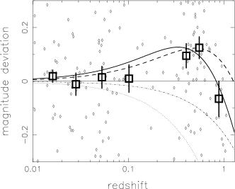
Figure 17: Literature supernovae (diamonds) shown along with median values binned by redshift (large squares). Individual points are shown without error bars for clarity. The solid horizontal line represents the empty universe with $(\Omega_{0{\rm m}},\Omega_{\Lambda})=(0.0,0.0)$. The thick solid line represents the magnitude deviation of our best-fit universe for this data-set from the empty universe. The thick dashed line represents $\Lambda$CDM with $(\Omega_{0{\rm m}},\Omega_{\Lambda})=(0.3,0.7)$, the dot-dashed and dotted lines represent cosmologies with $(\Omega_{0{\rm m}},\Omega_{\Lambda})=(0.3,0.0)\ {\rm and}\ (1.0,0.0)$ respectively.

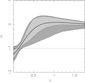
Figure 18: The evolution of $w(z)$ with redshift for $\Omega_{0{\rm m}}=0.3$. The reconstruction is done using the polynomial fit to dark energy, equation (7), for the latest HZT sample of 194 type Ia SNe. The thick solid line shows the best-fit, the light grey contour represents the $1\sigma$ confidence level, and the dark grey contour represents the $2\sigma$ confidence level around the best-fit. The dashed line represents $\Lambda$CDM. No priors are assumed on $w(z)$.

3 The accelerating universe and the Energy Conditions

The energy conditions :

• Strong energy condition: $\rho+3p\geq 0$ (SEC),

• Weak energy condition: $\rho\geq 0$, $\rho+p\geq 0$ (WEC)

play a vitally important role in our understanding of the accelerating universe, both in the context of inflation and dark energy. We therefore consider it worthwhile to review certain key developments which deepened our understanding of these issues.

In an expanding FRW universe the SEC implies that the universe decelerates while the WEC forbids the pressure from becoming too negative. Additionally, in the 1960’s and early 1970’s it was noted that energy conditions play a crucial role in the formulation of the singularity theorems in cosmology. Indeed, one of the necessary conditions for the existence of an initial/final singularity in big bang cosmology is that matter satisfies both the SEC and WEC (Hawking & Ellis, 1973).

By the late 1970’s it became clear that not all forms of matter satisfy the energy conditions. Perhaps the best example of a form of matter which satisfied the weak energy condition but violated the strong one is the cosmological constant, introduced into cosmology by Einstein in 1917. In addition, the vacuum expectation value of the energy momentum tensor, $\langle T_{ik}\rangle_{\rm vac}$, which describes quantum effects (particle production and vacuum polarization) in an expanding universe could, in certain cases, violate both WEC and SEC (Birrell & Davies, 1982; Grib, Mamaev & Mostepanenko, 1980). (For certain space-times, such as de Sitter space, the vacuum energy momentum tensor generates a cosmological constant since $\langle T_{ik}\rangle_{\rm vac}=\Lambda g_{ik}$.) Thus by the late 1970’s it was well known that neither of the energy conditions could be held as being sacrosanct.

The 1980’s, as we all know, led to great advances in the development of the inflationary paradigm. The inflaton field mimics the behaviour of a cosmological constant over sufficiently small intervals of time and therefore violates the SEC. Early dark energy models were based on inflaton-type scalars which coupled minimally to gravity (quintessence). Quintessence violates the SEC but respects the WEC. Precisely because of the latter property, not any experimentally obtained $d_{L}(z)$ is compatible with quintessence, as emphasized in Sahni & Starobinsky (2000). (The same observation holds for $H(z)$, since the latter can be derived from $d_{L}(z)$ using equation (3).) Clearly if observations do indicate that the WEC is violated by DE then more general (WEC-violating) models for DE should be seriously considered. One example of WEC-violating DE is provided by scalar-tensor gravity. Scalar-tensor models contain at least two functions of the scalar field (dilaton) describing dark energy. As shown in Boisseau et al.  (2000), these two functions, namely, the scalar field potential and its coupling to the Ricci scalar $R$, are sufficiently general to explain any $H(z)$ obtained from observations.

The WEC can also be effectively violated in DE models constructed in braneworld cosmology. It has recently been shown that such models, with $w_{\rm eff}<-1$, are in excellent agreement with supernova data (Alam & Sahni, 2002). Since the field equations in these models are derived from a higher dimensional Lagrangian the unusually rapid acceleration of the four dimensional universe arises because of the full five dimensional theory and not because of matter which continues to satisfy the energy conditions and whose density remained finite and well behaved at all times (Sahni & Shtanov, 2003). This behaviour is in contrast to phantom, which assumes a conventional ‘perfect fluid’ form for the energy-momentum tensor and therefore contains pathological features such as an energy density which diverges in the future and a sound speed which is faster than that of light (Caldwell, 2002; Sahni & Shtanov, 2003).

The fact that the observed luminosity distance (derived from supernova observations) is better fit by dark energy violating the WEC than either quintessence or a cosmological constant was first noticed by Caldwell (2002). Caldwell called this ‘phantom energy’ and showed that larger values of $\Omega_{0{\rm m}}$ ($\Omega_{0{\rm m}}\lower 3.87495pt\hbox{ $\buildrel>\over{\sim}$}~{}0.2$) implied increasingly more negative values for the equation of state ($w\lower 3.87495pt\hbox{ $\buildrel<\over{\sim}$}~{}-1$) of phantom. Caldwell’s results have since been confirmed by larger and better quality SNe data sets – for instance Knop et al.  (2003) find that, in the absence of priors being placed on $\Omega_{0{\rm m}}$, the DE equation of state has a $99\%$ confidence limit of being $<-1$ ! Both Caldwell (2002) and Knop et al.  (2003) however work under the assumption that the equation of state of dark energy is unevolving, so that $w=$ constant.

In this paper we have shown that, suspending the WEC prior and allowing the dark energy equation of state to evolve brings out dramatically new properties of dark energy. Thus the dark energy model which best fits the SNe observations has an equation of state which rapidly evolves from $w(z)\lower 3.87495pt\hbox{ $\buildrel<\over{\sim}$}~{}-1$ at present ($z=0$) to $w(z)\simeq 0$ at $z\sim 1$. Dark energy therefore appears to have properties which interpolate between those of dark matter (dust) at early times and those of a ‘phantom’ ($w\lower 3.87495pt\hbox{ $\buildrel<\over{\sim}$}~{}-1$) at late times.

4 Conclusions and discussion

This paper reports the model independent reconstruction of the cosmic equation of state of dark energy in which no priors are imposed on $w(z)$. In the literature the imposition of various priors frequently precedes the analysis of observational data sets. Such a procedure is well founded and entirely justified when priors are dictated by complementary information such as orthogonal observations coming from different data sets. However, on occasion the use of priors is justified on ‘theoretical grounds’ and in this case one must be careful so as not to prejudge nature. (Compelling theoretical reasons might well reflect our own particular conditioning or set of prejudices !) In the case of the analysis of type Ia supernova data, the priors most frequently used have been $w=$ constant and $w\geq-1$. Both confine DE to within a narrow class of models. Moreover, as shown in Maor et al.  (2002), the imposition of such priors on the cosmic equation of state can, on occasion, lead to gross misrepresentations of reality.

In this paper we do not impose any priors on $w(z)$ and reconstruct the equation of state of dark energy in a model independent manner. In this case our best fit $w(z)$ evolves from $w\lower 3.87495pt\hbox{ $\buildrel<\over{\sim}$}~{}-1$ at $z=0$, to $w\simeq 0$ at $0.8\lower 3.87495pt\hbox{ $\buildrel<\over{\sim}$}~{}z\lower 3.87495pt\hbox{ $\buildrel<\over{\sim}$}~{}1.75$ (the upper limit is set by observations). This result is robust to changes in the value of $\Omega_{0{\rm m}}$ and remains in place within the broad interval $0.1\leq\Omega_{0{\rm m}}\leq 0.5$. Our reconstruction clearly favours a model of DE whose equation of state metamorphoses from $w=0$ in the past to $w\simeq-1$ today. An excellent example of a model which has this property is the Chaplygin gas (Kamenshchik, Moschella & Pasquier, 2001). However, in this model dark energy does not violate the weak energy condition (if it was not already violated initially). Our results also lend support to the dark energy models discussed in Bassett et al.  (2002); Corasaniti et al.  (2003) in which the DE equation of state shows a late-time phase transition. An interesting example of an evolving DE model in which $w_{0}<-1$ at present whereas $w(z)>-1$ at earlier times is provided by the braneworld models (called BRANE1) examined in Sahni & Shtanov (2003) which have been shown to agree very well with current supernova observations (Alam & Sahni, 2002).

It is also conceivable that the observed rapid growth in the EOS might characterise ‘unified’ models of dark matter (DM) and dark energy (DE). We end this paper with a small speculation on this last possibility. Since the nature of both DM and DE is currently unknown, it may be that a mechanism exists which converts DM (with $w=0$) into DE (with $w\simeq-1$) in regions with sufficiently high density contrast $\delta\rho/\rho\gg 1$. (This would happen if, for instance, the rate of conversion of DM into DE depended upon $(\delta\rho/\rho)^{x},x\gg 1$, etc.) Since the conversion of DM to DE is confined to high peaks of the density field this process will not occur uniformly in the entire universe but will be restricted to regions occupying a small filling fraction ($FF$) ($FF\ll 1$ for regions with $\delta\rho/\rho\gg 1$; see for instance Sheth et al.  (2003) and references therein). This process could commence as early as $z\sim 10-20$ when the first peaks in a CDM model collapse. Since DE does not cluster and since $\rho_{\rm DE}/\rho_{\rm DM}$ grows rapidly as the universe expands, DE from high density regions ($FF\ll 1$) will spread at the speed of light, percolating through the entire universe ($FF\sim 1$) by $z\sim 1$. Since the creation of DE is tagged to the formation of structure, this model may not encounter the ‘coincidence problem’ which plagues other scenarios of DE including quintessence. (However this model might have problems in producing a sufficiently homogeneous and isotropic distribution of dark energy on the largest scales.) The concrete mathematical framework for a phenomenological model of this kind will be worked out in a companion paper.

In summary, evolving DE models have been shown to satisfy SNe observations just as well (if not better) than the cosmological constant. Our best fit equation of state, in the absence of any priors, evolves from $w(z)\lower 3.87495pt\hbox{ $\buildrel<\over{\sim}$}~{}-1$ at $z=0$ to $w(z)\simeq 0$ at $z\sim 1$. Indeed, figure 17 shows that our best fit EOS is better able to account for the relative brightness of supernovae at $z\lower 3.87495pt\hbox{ $\buildrel>\over{\sim}$}~{}0.8$ than $\Lambda$CDM. However, the evolution in $w(z)$ is much weaker if the prior $w(z)\geq-1$ ($z\geq 0$) is imposed. Due to the paucity of SNe data beyond $z=1.2$ (till date, there is only a single data point beyond $z=1.2$, SN1999bf at $z=1.75$) it is not clear whether $w(z)\simeq 0$ is a stable asymptotic value for the reconstructed DE equation of state at high redshifts. New supernova data at $z\lower 3.87495pt\hbox{ $\buildrel>\over{\sim}$}~{}1$ from ongoing as well as planned surveys (SNAP) combined with data from other cosmology experiments (CMB, LSS, S-Z survey’s, lensing, etc.) are bound to provide important insights on the nature of dark energy at high redshifts. Our results clearly throw open exciting new possibilities for dark energy model building.

Acknowledgments:

We would like to thank John Tonry for several important clarifications and for help in preparing figure 17. We also thank Sarah Bridle, Pier-Stefano Corasaniti, Alessandro Melchiorri, Yuri Shtanov and Lesha Toporenskii for their useful comments on an earlier version of the paper. One of us (VS) acknowledges useful discussions with Salman Habib and Daniel Holz.

UA thanks the CSIR for providing support for this work. AS was partially supported by the Russian Foundation for Basic Research, grant 02-02-16817, and by the Research Program “Astronomy” of the Russian Academy of Sciences.

Appendix A Propagation of errors

We have seen that the error bars on $w(z)$ for the analysis using ansatz (7) are non-monotonic with redshift. Low redshift behaviour of the equation of state affects the luminosity distance at all higher redshifts, while high redshift behaviour effects fewer such distances. This leads to an expectation that high-$z$ behaviour of the equation of state should be poorly constrained as opposed to the low-$z$ behaviour. This seems to contradict the behaviour seen in our figures. To investigate if this could be explained by our specific method of error analysis we describe the Fisher matrix error bars below and show that they are almost identical to what we obtain in our method.

In an analysis which uses an ansatz with $n$ parameters $p_{i}$, the Fisher information matrix is defined to be

$$F_{ij}\equiv\left\langle\frac{\partial^{2}{\bf L}}{\partial p_{i}\partial p_{j}}\right\rangle\,\,,$$ (26)

where ${\bf L}=-{\rm log}\cal{L}$, $\cal{L}$ being the likelihood . For an unbiased estimator, the errors on the parameters will follow the Cramér-Rao inequality : $\Delta p_{i}\geq 1/\sqrt{F_{ii}}$.

Since the likelihood function is approximately Gaussian near the maximum likelihood (ML) point, the covariance matrix for a maximum likelihood estimator is given by

$$(C^{-1})_{ij}\equiv\frac{\partial^{2}{\bf L}}{\partial p_{i}\partial p_{j}}\,\,.$$ (27)

The Fisher information matrix is therefore simply the expectation value of the inverse of the covariance matrix at the ML-point.

Given the covariance matrix, the error on any cosmological quantity $Q(p_{i})$ is given by :

$$\sigma_{Q}^{2}=\sum_{i=1}^{n}\left(\frac{\partial Q}{\partial p_{i}}\right)^{2}C_{ii}+2\sum_{i=1}^{n}\sum_{j=i+1}^{n}\left(\frac{\partial Q}{\partial p_{i}}\right)\left(\frac{\partial Q}{\partial p_{j}}\right)C_{ij}\,\,.$$ (28)

Thus the nature of the errors on a quantity will depend essentially on the manner in which it is related to the parameters of the system.

We now consider how errors propagate for different cosmological quantities for the polynomial fit to dark energy which we have used for most of the results in this paper :

$$H^{2}/H_{0}^{2}=\Omega_{0{\rm m}}x^{3}+A_{0}+A_{1}x+A_{2}x^{2},~{}x=1+z\,\,,$$ (29)

where $A_{0}=1-\Omega_{0{\rm m}}-A_{1}-A_{2}$. If $\Omega_{0{\rm m}}$ is held constant then the parameters of the system are $(A_{1},A_{2})$.

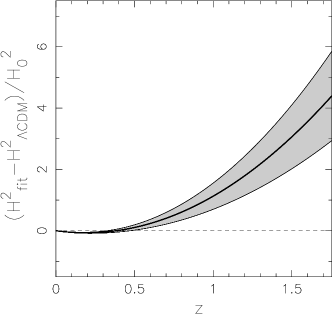
Figure 19: The deviation of $H^{2}/H_{0}^{2}$ from corresponding $\Lambda$CDM values over redshift for the ansatz (7). The thick solid line shows the best-fit and the light grey contour represents the $1\sigma$ confidence level around the best-fit. The dashed horizontal line denotes $\Lambda$CDM. $\Omega_{0{\rm m}}=0.3$ is assumed.

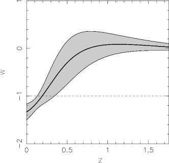
Figure 20: The variation of the equation of state of dark energy $w(z)$ over redshift for the ansatz (7). The thick solid line shows the best-fit and the light grey contour represents the $1\sigma$ confidence level around the best-fit. The dashed horizontal line denotes $\Lambda$CDM. $\Omega_{0{\rm m}}=0.3$ is assumed.

We obtain the covariance matrix in $(A_{1},A_{2})$ from the ML analysis, and then using equation (28), calculate the errors on cosmological quantities of interest. For example, the errors on the quantity $\Delta H^{2}=(H^{2}-H^{2}_{\Lambda CDM})/H_{0}^{2}$ are given by :

$$\sigma_{\Delta H^{2}}^{2}(x)=(x-1)^{2}[C_{11}+2(x+1)C_{12}+(x+1)^{2}C_{22}]\,\,.$$ (30)

Although the term $C_{12}$ is negative we find that $\sigma_{\Delta H^{2}}^{2}(x)$ still increases with redshift. This is shown in the figure 19. The errors shown are approximately similar to those obtained in figure 3.

The corresponding errors on the equation of state can be calculated using equations (18) and (28), and has the somewhat more complicated expression :

$$\sigma_{w}^{2}(x)=\frac{x^{2}[f_{1}^{2}C_{11}+2f_{1}f_{2}C_{12}+f_{2}^{2}C_{22}]}{9[1-\Omega_{0{\rm m}}+A_{1}(x-1)+A_{2}(x^{2}-1)]^{4}}\,\,,$$ (31)

where

$$f_{1} = 1-\Omega_{0{\rm m}}-A_{2}(x-1)^{2}~{},$$

$$f_{2} = 2x(1-\Omega_{0{\rm m}})+A_{1}(x-1)^{2}\,\,,$$

and $A_{1},A_{2}$ are the mean values of the parameters. Although in this case it is difficult to predict the behaviour of error bars, after substituting the numerical values we obtain the error bars that are shown in figure 20. This figure can be compared to the figure 5(b), having almost identical errors.

This shows that the nature of our error bars is not an artifact of our specific method of error analysis. However, as shown in figure 15, a two parameter expansion in $w(z)$ shows monotonically deteriorating errors in $w(z)$ with the redshift, while the expansion in $H_{2}(z)$ shows errors that improve with redshift (figure 5(b)). This indicates that the nature of error bars might be affected by which quantity is being approximated. In the limit of infinite terms in the expansion of various quantities all the methods should produce identical result. The practical need for truncating these expansions make these approximations slightly different from each other. More specifically, we require setting of priors

$$f(z) = \sum_{i=0}^{\infty}a_{n}z^{n}$$ (32)

$$a_{n} = 0;\ (n>N_{p})$$ (33)

where $f(z)$ could be $H(z)$, $w(z)$ or any other physical quantity and $N_{p}$ is the chosen number of parameters. The non-linear priors in the above equation make different finite expansions inequivalent. Since we do not know for certain if the underlying model for the accelerating expansion involves an energy component with negative pressure in a FRW setting we are forced to choose one of the alternatives for approximations. We hope that with increasingly high quality data the effect of such truncations will eventually disappear.

Appendix B Reconstruction of Other Dark Energy Models

$\begin{array}[]{c@{\hspace{0.4in}}c}\lx@intercol\mbox{}\hfil\lx@intercol&\lx@intercol\mbox{}\hfil\lx@intercol\\[0.0pt] \epsfbox{h_exp_error_lin.epsi}\hfil\hskip 28.90755pt&\epsfbox{h_exp_error_coras.epsi}\\ \mbox{\bf(a)}\hfil\hskip 28.90755pt&\mbox{\bf(b)}\end{array}$

Figure 21: The deviation $\Delta{\rm log}(d_{L}H_{0})/{\rm log}(d_{L}H_{0})$ between actual value and that calculated using the ansatz (7) over redshift for different values of parameters for (a) the Linder fit, and (b) the Corasaniti fit for equation of state of dark energy, with $\Omega_{0{\rm m}}=0.3$. In panel (a), the solid line shows the deviation for the Linder fit with $w_{0}=-0.8,w_{1}=0.5$, the dotted line for $w_{0}=-1.0,w_{1}=1.0$, and the dot-dashed line for $w_{0}=-1.2,w_{1}=2.0$. In panel (b), the solid line represents the Corasaniti fit with $w_{Q}^{0}=-0.8,w_{Q}^{m}=-0.5,z_{c}^{m}=1.5,\Delta=0.1$, the dotted line shows $w_{Q}^{0}=-1,w_{Q}^{m}=-0.2,z_{c}^{m}=0.6,\Delta=0.07$, and the dot-dashed line, $w_{Q}^{0}=-1.2,w_{Q}^{m}=0.1,z_{c}^{m}=0.11,\Delta=0.03$. The dashed horizontal line in both panels represents zero deviation from model values, which is true for $\Lambda$CDM, and $w=-1/3,w=-2/3$ quiessence models.

We have seen in the figure 1 that the ansatz (7) works well for several physically motivated models of quintessence, Chaplygin gas and SUGRA. In this section we take this exercise further and see how well it can reconstruct some of the other fits to dark energy known in literature. In figures 21 (a) and (b), we show results for simulations using $\Omega_{0{\rm m}}=0.3$ and two different fits to the equation of state of dark energy :

(a) The fit suggested in Linder (2003) : $w(z)=w_{0}+w_{1}z/(1+z)$. For this we consider three sets of values in order of increasing evolution of $w(z)$ : (a) $w_{0}=-0.8,w_{1}=0.5$, (b) $w_{0}=-1.0,w_{1}=1.0$, and (c) $w_{0}=-1.2,w_{1}=2.0$, and,

(b) The non-perturbative $w(z)$ suggested in Corasaniti & Copeland (2003) and Corasaniti et al.  (2003), which has the parameters $w_{Q}^{0}$ (the dark energy equation of state today), $w_{Q}^{m}$ (the dark energy equation of state at the matter dominated epoch), $z_{c}$ (the redshift where equation of state changes from $w_{Q}^{m}$ to $w_{Q}^{0}$), and $\Delta$ (the width of transition). For the simulation we again use three sets of values in order of increasing growth rate of $w(z)$ : (a) $w_{Q}^{0}=-0.8,w_{Q}^{m}=-0.5,z_{c}^{m}=1.5,\Delta=0.1$, (b) $w_{Q}^{0}=-1.0,w_{Q}^{m}=-0.2,z_{c}^{m}=0.6,\Delta=0.07$, and (c) $w_{Q}^{0}=-1.2,w_{Q}^{m}=0.1,z_{c}^{m}=0.11,\Delta=0.03$.

We find that in both cases, the ansatz recovers the measured quantity to within $0.5\%$ accuracy in the redshift range important for SNe observations. Thus we find that even for fits for which the ansatz does not return exact values, it can recover cosmological quantities to a high degree of accuracy.

References

- Alam & Sahni (2002) Alam, U. and Sahni, V., 2002, astro-ph/0209443.
- Alam, Sahni & Starobinsky (2003) Alam, U., Sahni, V. and Starobinsky, A.A., 2003, JCAP 0304, 002, [astro-ph/0302302].
- Alam et al. (2003) Alam, U., Sahni, V., Saini, T. D., and Starobinsky, A.A., 2003, Mon. Not. Roy. Ast. Soc. , 344, 1057 [astro-ph/0303009].
- Alcaniz, Jain and Dev (2002) Alcaniz, J.S., Jain. D. and Dev, A., 2002, Phys. Rev. D 66, 067301 [astro-ph/0206448].
- Amendola (2000) Amendola, L., 2000, Phys. Rev. D 62, 043511.
- Barber et al. (2000) Barber, A.J., et al. , 2000, Astroph. J. 545, 444.
- Barris et al. (2003) Barris, B. J. et al. , 2004, Astroph. J. 602, 571B [astro-ph/0310843].
- Bartolo & Pietroni (2000) Bartolo, N. and Pietroni, M. 2000 Phys. Rev. D 61, 023518.
- Bassett et al. (2002) Bassett, B.A., Kunz, M., Silk, J. and Ungarelli, C., 2002, MNRAS, 336, 1217 [astro-ph/0203383].
- Bertolami & Martins (2000) Bertolami, O. and Martins, P.J., 2000, Phys. Rev. D 61, 064007.
- Birrell & Davies (1982) Birrell, N.D. & Davies, P.C.W., 1982, Quantum Fields in Curved Space, Cambridge University Press, Cambridge.
- Boisseau et al. (2000) Boisseau, B., Esposito-Farese, G., Polarski, D. and Starobinsky, A.A., 2000, Phys. Rev. Lett. 85, 2236
- Caldwell, Dave & Steinhardt (1998) Caldwell, R.R., Dave, R. and Steinhardt, P.J., 1998, Phys. Rev. Lett. 80, 1582.
- Caldwell (2002) Caldwell, R.R., 2002, Phys. Lett. B 545, 23 [astro-ph/9908168].
- Caldwell, Kamionkowski & Weinberg (2003) Caldwell, R.R., Kamionkowski, M. and Weinberg, N.N., 2003, Phys.Rev.Lett. 91 071301 [astro-ph/0302506].
- Carroll (2001) Carroll, S.M., 2001, Living Rev.Rel. 4 1 [astro-ph/0004075].
- Carroll, Hoffman & Trodden (2003) Carroll, S.M., Hoffman, M. and Trodden, M., 2003, Phys. Rev. D 68, 023509 [astro-ph/0301273].
- Cayrel et al. (2001) Cayrel, R. et al. , 2001, Nature 409, 691 [astro-ph/0104357].
- Chaboyer & Krauss (2002) Chaboyer, B. and Krauss, L.M., 2002, ApJ, 567, L45.
- Chiba & Nakamura (2000) Chiba, T. and Nakamura, T., 2000, Phys. Rev. D 62, 121301(R).
- Chiba, Okabe, & Yamaguchi (2000) Chiba, T., Okabe, T. and Yamaguchi, M, 2000, Phys. Rev. D 62, 023511.
- Chimento et al. (2003) Chimento, L.P., Jakubi, A.A., Pavon, D. and Zimdahl, W., 2003, Phys. Rev. D 67 083513 [astro-ph/0303145].
- Copeland, Liddle & Lidsey (2001) Copeland, E.J., Liddle, A.R. and Lidsey, J.E., 2001, Phys. Rev. D 64 023509.
- Corasaniti & Copeland (2003) Corasaniti, P.S. and Copeland, E.J., 2003, Phys. Rev. D 67 063521 [astro-ph/0205544].
- Corasaniti et al. (2003) Corasaniti, P.S., Bassett, B.A., Ungarelli, C. and Copeland, E.J., 2003, Phys. Rev. Lett. 90, 091303 [astro-ph/0210209].
- Daly & Djorgovsky (2003) Daly, R.A. and Djorgovsky, S.G., 2003, Astroph. J. 597, 9-20. [astro-ph/0305197].
- Damour, Kogan & Papazoglou (2002) Damour, T., Kogan, I.I. and Papazoglou, A., 2002, Phys. Rev. D 66, 104025 [hep-th/0206044].
- Deffayet, Dvali & Gabadadze (2002) Deffayet, C., Dvali, G. and Gabadadze, G., 2002, Phys. Rev. D 65, 044023 [astro-ph/0105068].
- Felder et al. (2002) Felder, G.N., Frolov, A., Kofman, L. and Linde, A., 2002, Phys. Rev 66, 023507.
- Frampton (2003) Frampton, P., 2003, Phys. Lett. B 555, 139.
- Frampton & Takahashi (2003) Frampton, P. and Takahashi, T., 2003, Phys. Lett. B 557, 135.
- Freedman et al. (2001) Freedman, W., et al. , 2001, Astroph. J. 553, 47.
- Gerke & Efstathiou (2002) Gerke, B, & Efstathiou, G., 2002, Mon. Not. Roy. Ast. Soc. 335 33, [astro-ph/0201336].
- Gnedin, Lahav & Rees (2001) Gnedin, N, Lahav, O. and Rees, M.J., astro-ph/0108034.
- Gratton et al. (2003) Gratton, R. et al. , 2003, A& A, 408, 529, [astro-ph/0307016].
- Grib, Mamaev & Mostepanenko (1980) Grib, A.A., Mamaev, S.G. and Mostepanenko, V.M., 1980, Quantum Effects in Strong External Fields, Moscow, Atomizdat (in Russian) [English translation: Vacuum Quantum Effects in Strong Fields, Friedmann Laboratory Publishing, St.Petersburg, 1994].
- Hansen et al. (2002) Hansen, B. et al. , 2002, ApJ 574, L155.
- Hawking & Ellis (1973) Hawking, S.W. and Ellis, G.F.R., 1973, The large scale structure of space-time, Cambridge University Press.
- Hoffman (2003) Hoffman, M., 2003, astro-ph/0307350.
- Huterer & Starkman (2002) Huterer, D. and Starkman, G., 2003, Phys. Rev. Lett. 90, 031301, [astro-ph/0207517].
- Huterer & Turner (1999) Huterer, D. and Turner, M.S., 1999, Phys. Rev. D , 60, 081301.
- Johri (2003) Johri, V.B., 2003, astro-ph/0311293.
- Kallosh et al. (2002) Kallosh, R., Linde, A., Prokushkin, S. and Shmakova, M., 2002, Phys. Rev. D 66 123503.
- Kamenshchik, Moschella & Pasquier (2001) Kamenshchik, A., Moschella, U. and Pasquier, V., 2001, Phys. Lett. B 511 265.
- Knop et al. (2003) Knop, R.A., et al., 2003, Astroph. J. 598 102 [astro-ph/0309368].
- Krauss (2001) Krauss, L.M., 2001, in Proceedings, ESO-CERN-ESA Symposium on Astronomy, Cosmology and Fundamental Physics, March 2002.
- Krauss (2001) Krauss, L.M., 2001, in International Conference on the identification of Dark Matter, Eds. N. Spooner and V. Kudryavtsev (Singapore, World Scientific), 1.
- Krauss & Chaboyer (2001) Krauss, L.M. and Chaboyer, B., 2001, astro-ph/0111597.
- Kunz et al. (2003) Kunz, M., Corasaniti, P., Parkinson, D. and Copeland, E.J., 2003, astro-ph/0307346.
- Linder (2003) Linder, E.V., 2003, Phys. Rev. Lett. 90 091301, [astro-ph/0208512].
- Maeda, Mizuno & Torii (2003) Maeda, K., Mizuno, S. and Torii, T., 2003, Phys. Rev. D 68 024033 [gr-qc/0303039].
- Maor et al. (2002) Maor, I. et al. , 2002, Phys. Rev. D 65 123003, [astro-ph/0112526].
- Marchi et al. (2003) Marchi, G. De, et al. , 2004, Astron. Astrophys. 415, 971 [astro-ph/0310646].
- McInnes (2002) McInnes, B., 2002, JHEP 0208, 029 [hep-th/0112066].
- Nakamura & Chiba (1999) Nakamura, T. and Chiba, T., 1999, Mon. Not. Roy. Ast. Soc. , 306, 696.
- Nunes & Lidsey (2003) Nunes, N.J. and Lidsey, J.E., 2003, astro-ph/0310882.
- Padmanabhan (2003) Padmanabhan, T., 2003, Phys. Rep. 380, 235 [hep-th/0212290].
- Parker & Raval (1999) Parker, L. and Raval, A., 1999, Phys. Rev. D 60, 063512, 123502.
- Peebles & Ratra (1988) Peebles, P.J.E. and Ratra, B., 1998, Ap. J. Lett. 325, L17.
- Peebles & Ratra (2002) Peebles, P.J.E. and Ratra, B., 2002, Rev.Mod.Phys. 75, 559 [astro-ph/0207347].
- Peebles & Vilenkin (1999) Peebles, P.J.E. and Vilenkin, A., 1999 Phys. Rev. D 59 063505.
- Percival et al. (2001) Percival, W.J., et al. , 2001, Mon. Not. Roy. Ast. Soc. 327, 1297.
- Perlmutter et al. (1999) Perlmutter, S.J., et al. , 1999, Astroph. J. 517, 565.
- Riess et al. (1998) Riess, A.G., et al. , 1998, Astron. J. 116, 1009.
- Sahni (2002) Sahni, V., 2002, Class. Quantum Grav. 19, 3435, [astro-ph/0202076].
- Sahni & Habib (1998) Sahni, V. and Habib, S., 1998, Phys. Rev. Lett. 81, 1766, [hep-ph/9808204].
- Sahni et al. (2003) Sahni, V., Saini, T.D., Starobinsky, A.A. and Alam, U., 2003, JETP Lett. 77 201 [astro-ph/0201498].
- Sahni, Sami & Souradeep (2002) Sahni, V., Sami, M. and Souradeep, T., 2002, Phys. Rev. D 65 023518.
- Sahni & Shtanov (2003) Sahni, V. and Shtanov, Yu.V., 2003, JCAP 11 014, [astro-ph/0202346].
- Sahni & Starobinsky (2000) Sahni, V. and Starobinsky, A.A., 2000, IJMP D 9, 373 [astro-ph/9904398].
- Sahni & Wang (2000) Sahni, V. and Wang, L., 2000, Phys. Rev. D 62, 103517 [astro-ph/9910097].
- Saini (2003) Saini, T.D., 2003, Mon. Not. Roy. Ast. Soc. 344, 129.
- Saini et al. (2000) Saini, T.D., Raychaudhury, S., Sahni, V. and Starobinsky, A.A., 2000, Phys. Rev. Lett. , 85, 1162.
- Sheth et al. (2003) Sheth, J.V., Sahni, V., Shandarin, S.F. and Sathyaprakash, B.S., 2003, MNRAS 343, 22 [astro-ph/0210136].
- Singh, Sami & Dadhich (2003) Singh, P., Sami, M. and Dadhich, N.K., 2003, Phys. Rev. D 68, 023522 [hep-th/0305110].
- Spergel et al. (2003) Spergel, D.N. et al. , 2003, Astroph. J. Suppl. 148, 175 [astro-ph/0210136]
- Starobinsky (1998) Starobinsky, A.A., 1998, JETP Lett. 68, 757.
- Tegmark (2002) Tegmark, M., 2002, Phys. Rev. D 66, 103507.
- Tegmark et al. (2003) Tegmark, M., et al. 2003, astro-ph/0310723.
- Thompson et al. (2001) Thomson, I.B. et al. , 2001, Astron. J. 121, 3089.
- Tonry et al. (2003) Tonry, J.L., et al., 2003, Astroph. J. 594, 1, [astro-ph/0305008].
- Urena-Lopez & Matos (2000) Urena-Lopez, L.A., Matos, T., 2000, Phys. Rev. D 62, 081302, [astro-ph/0003364].
- Wang & Lovelace (2001) Wang, Y and Lovelace, G, 2001, Astroph. J. 562, L115.
- Weinberg (1989) Weinberg, S. (1989) Rev. Mod. Phys. 61, 1.
- Weller & Albrecht (2002) Weller, J. and Albrecht, A., 2002, Phys. Rev. D 65, 103512 [astro-ph/0106079].
- Wetterich (1988) Wetterich, C, 1988, Nucl. Phys. B302, 668.
- Zeldovich (1968) Zeldovich, Ya.B. (1968) Sov. Phys. – Uspekhi 11, 381.