The Size of the Longest Filaments in the Universe

Abstract

We analyze the filamentarity in the Las Campanas redshift survey (LCRS) and determine the length scale at which filaments are statistically significant. The largest length-scale at which filaments are statistically significant, real objects, is between $70$ to $80\,h^{-1}$Mpc, for the LCRS $-3^{o}$ slice. Filamentary features longer than $80\,h^{-1}$Mpc, though identified, are not statistically significant; they arise from chance alignments. For the five other LCRS slices, filaments of lengths $50\,h^{-1}$Mpc to $70\,h^{-1}$Mpc are statistically significant, but not beyond. These results indicate that while individual filaments up to $80\,h^{-1}$Mpc are statistically significant, the impression of structure on larger scales is a visual effect. On scales larger than $80\,h^{-1}$Mpc the filaments interconnect by statistical chance to form the the filament-void network. The reality of the $80\,h^{-1}$Mpc features in the $-3^{o}$ slice make them the longest coherent features in the LCRS. While filaments are a natural outcome of gravitational instability, any numerical model attempting to describe the formation of large scale structure in the universe must produce coherent structures on scales that match these observations.

1 Introduction

One of the most striking visual features in the distribution of galaxies in the Las Campanas redshift Survey (LCRS, Shectman et al. 1996) is that they appear to be distributed along filaments. These filaments are interconnected and form a network, with voids largely devoid of galaxies comprising the region in between the filaments. This network of interconnected filaments encircling voids extends across the entire survey and may be referred to as the “Cosmic Web”. Similar networks of filaments and voids are also visible in other galaxy surveys, e.g., CfA (Geller & Huchra 1989), 2dFGRS (Colless et al. 2001, Colless et al. 2003) and SDSS (EDR) (Stoughton et al. 2002, Abazajian et al. 2003). These, if they are a genuine feature of the galaxy distribution, represent the largest structural elements in the hierarchy of structures observed in the universe, namely galaxies, clusters, superclusters, filaments and the cosmic web.

The analysis of filamentary patterns in the galaxy distribution has a long history dating back to papers by Zel’dovich, Einasto and Shandarin (1982), Shandarin and Zel’dovich (1983) and Einasto et al. (1984). In the last paper the authors analyze the distribution of galaxies in the Local Supercluster. They use the Friend-of-Friend algorithm with varying neighborhood radius to identify connected systems of galaxies referred to as “clusters”. As they increase the neighborhood radius, they find that the clusters which are initially spherical become multi-branched with multiple filaments of lengths up to several tens of $h^{-1}$Mpc extending out in different directions. Finally, as the radius is increased further, they find that the filaments get interconnected and join neighboring superclusters into an infinite network of superclusters and voids. A later study (Shandarin & Yess 2000) used percolation analysis to arrive at a similar conclusion for the distribution of the LCRS galaxies. The large-scale and super large-scale structures in the distribution of the LCRS galaxies have also been studied by Doroshkevich et al. (2001) and Doroshkevich et al. (1996) who find evidence for a network of sheet like structures which surround underdense regions (voids) and are criss-crossed by filaments. The distribution of voids in the LCRS has been studied by Müller, Arbabi-Bidgoli, Einasto & Tucker (2000) and the topology of the LCRS by Trac, Mitsouras, Hickson & Brandenberger (2002) and Colley (1997). A recent analysis (Einasto et al. 2003a) indicates a supercluster-void network in the Sloan Digital Sky Survey also.

Traditionally, correlation functions (Peebles 1993) have been used to quantify the statistical properties of the galaxy distribution. For the LCRS, the two-point correlation function is a power law,

$$\xi(r)=\left({r\over r_{o}}\right)^{-1.52}$$ (1)

with the correlation length $r_{o}=6.28$ $h^{-1}$Mpc on scales $2.0\,h^{-1}$Mpc to $16.4\,h^{-1}$Mpc. On scales larger than $30-40\,h^{-1}$Mpc, $\xi$(r) fluctuates closely around zero indicating a statistically homogeneous galaxy distribution at and beyond these scales (Tucker et al. 1997). This raises the question whether the filamentary features which appear to span scales larger than $100\,h^{-1}$Mpc are statistically significant features of the galaxy distribution or if they are mere artifacts arising from chance alignment of the galaxies.

A quantitative estimator of filamentary structure, Shapefinder, was defined (Bharadwaj et al. 2000) to provide a measure of the average filamentarity for a point distribution in 2D. (See Sahni, Sathyaprakash & Shandarin 1998 for general introduction to Shapefinders and Sheth et al. 2003 for the application of Shapefinders to 3D simulations of structure formation.) The Shapefinder statistic was used to demonstrate that the galaxy distribution in the LCRS exhibits a high degree of filamentarity compared to a random Poisson distribution having the same geometry and selection effects as the survey. This analysis provides objective confirmation of the visual impression that the galaxies are distributed along filaments. This, however, does not establish the statistical significance of the filaments. The features identified as filaments are essentially chains of galaxies, a crucial requirement being that the spacing between any two successive galaxies along a chain is significantly smaller than the mean inter-galaxy separation. A chain runs as long as it is possible to find another nearby galaxy which is not yet a member of the chain, and breaks when no such galaxy is to be found. The fact that the LCRS galaxies are highly clustered on small scales increases the probability of finding pairs of galaxies at small separations. This enhances the occurrence of long chains of galaxies, and we expect to find a higher degree of filamentarity arising just from chance alignments in the LCRS compared to a Poisson distribution. To establish whether the observed filaments are statistically significant or if they are a result of chance alignments of smaller structural elements, it is necessary to compare the sample of galaxies (here, the LCRS slices) with a distribution of points which has the same small scale clustering properties as the original sample and for which we know that all large-scale filamentary features are solely due to chance alignments. This is achieved using a statistical technique called Shuffle (Bhavsar & Ling 1988) whereby the statistical significance of the filamentarity in a clustered dataset can be assessed.

Shuffle generates fake data-sets, practically identical in their clustering properties to the original data up to a length scale $L$, but in which all structures longer than $L$, both real and chance, of the original data, have been eliminated. In these Shuffled data, filaments spanning length-scales larger than $L$ are visually evident, even expected to be identified as a signal by the statistics used to quantify the filamentarity, but all filaments spanning length-scales larger than L have formed accidentally. The measure of the occurrence of filaments spanning length-scales larger than $L$ in the Shuffled data gives us a statistical estimate of the level at which chance filaments spanning length-scales larger than $L$ occur in the original data. Here we use Shuffle to estimate the degree of filamentarity expected from chance alignments in the LCRS and use this to determine the statistical significance of the observed filamentarity.

We present the method of analysis and our findings in Section 2. In Section 3 we discuss our results and present conclusions.

2 Analysis and Results

The LCRS contains the angular positions and redshifts of 26,418 galaxies distributed in 6 wedges, each $1.5^{o}$ thick in declination and $80^{o}$ in right ascension. Three wedges are centered around mean declinations $-3^{o}$, $-6^{o}$ and $-12^{o}$ in the Northern galactic cap and three at declinations $-39^{o}$, $-42^{o}$ and $-45^{o}$ in the Southern galactic cap. The survey has a magnitude limit $m=17.75$ and extends to a distance of $600\,h^{-1}$Mpc. The most prominent visual feature in these wedges (Figure 1) is that the galaxies appear to be distributed along filaments, several of which span length-scales of $100\,h^{-1}$Mpc or more.

We extracted luminosity and volume limited sub-samples (Figure 1) from the LCRS data so that we have an uniform sampling of the regions that we analyze. In order to sample the largest regions that we could, with the above criterion in mind, we limited the wedges from $195$ to $375\,h^{-1}$Mpc in the radial direction as shown in Figure 1.

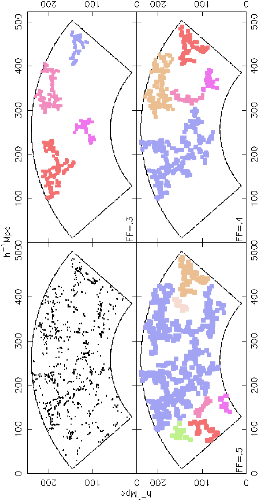
Figure 1: The upper left hand panel shows the distribution of galaxies in an uniformly sampled region of the $-3^{o}$ slice. The filamentary patterns of galaxies are evident. Going clockwise, the three other panels show some of the largest clusters identified using FOF after N=3,4 and 5 iterations of coarse-graining. Most of the clusters shown are highly filamentary (${\cal F}_{2}>0.8$), with ${\cal F}_{2}>0.9$ for the largest cluster in each panel (the definition of ${\cal F}_{2}$ is given in the text). At each level of coarse-graining, clusters grow until we have a single, large filamentary network spanning the whole region, referred to as the “Cosmic Web”.

Our data consist of a total of 5073 galaxies distributed in 6 wedges. Each LCRS wedge is collapsed along its thickness (in declination) resulting in a 2 dimensional truncated conical slice which, being geometrically flat, can be unrolled onto a plane. Each slice is embedded in a $1\,h^{-1}$Mpc $\times 1\,h^{-1}$Mpc rectangular grid. Grid cells with galaxies in them are assigned the value 1, empty cells 0. Connected regions of filled cells are identified as clusters using a “friends-of-friends”(FOF) algorithm. The geometry and topology of each cluster is described by its area $S$, perimeter $P$, and genus $G$. It is possible to utilize these measures to assess the filamentarity of the supercluster of interest. This is achievable using a set of measures termed as Shapefinders, originally defined for 2D hypersurfaces embedded in 3D. We use a 2D version of the Shapefinder in our analysis of the superclusters in the LCRS slices. However, before presenting our results, we digress briefly and summarize the definition and the conceptual foundation of the Shapefinder measures.

The geometry of a given structure is sensitive to any deformation which the structure undergoes, while the topology of the structure, solely relating to the connectedness of the structure, remains unaffected. The morphology and the size of the objects is a result of the interplay between both these aspects. The Shapefinders are statistics devised to utilize both geometric and topological information of a given object, to make a meaningful statement about its size and its morphology. Both the geometry and topology of an object are characterized in terms of Minkowski Functionals (hereafter MFs). In 3D, the geometric MFs are (1) the Volume ${\cal V}$, (2) the surface area ${\cal S}$ and (3) the integrated mean curvature ${\cal C}$, whereas the fourth MF is a topological invariant, the genus ${\cal G}$. Sahni et al. (1998) defined three Shapefinders as the ratio’s of the above MFs, so as to have the dimensions of length. These are conventionally considered to be reminiscent of the characteristic thickness ${\cal T}=3{\cal V/S}$, breadth ${\cal B}{\cal=S/C}$ and length ${\cal L}={\cal C}/4\pi({\cal G}+1$) of the object, and thus, together with genus ${\cal G}$, give us a feel for the typical size and topology of the object of interest. The information content about the three characteristic length-scales associated with the object can further be used to make an objective statement about the morphology of the object, as to how spherical, planar, ribbon-like or filamentary an object is. Sahni et al. (1998) proposed to achieve this by using two dimensionless Shapefinders, namely planarity ${\cal P}$ and Filamentarity ${\cal F}$ defined as follows:

$${\cal P}={{\cal B-T}\over{\cal B+T}};~{}~{}~{}{\cal F}={{\cal L-B}\over{\cal L+B}}.$$ (2)

These are defined so that for an ideal sheet like object, ${\cal P}$ = 1, ${\cal F}$ = 0, whereas for an ideal one-dimensional filament, ${\cal P}$ = 0, ${\cal F}$ = 1 ^,.

In our present analysis, we use the 2D version of the Shapefinders, the Shapefinder measure ${\cal F}$

$${\cal F}={({\cal P}^{2}-16{\cal S})\over({\cal P}-4)^{2}},$$ (3)

originally defined in Bharadwaj et al. (2000), to quantify the shape of the superclusters in the quasi-2D slices of the LCRS. By definition 0$\leq{\cal F}\leq$ 1. ${\cal F}$ quantifies the degree of filamentarity of a cluster, with ${\cal F}$ = 1 indicating a filament and ${\cal F}$ = 0, a square (while dealing with a density field defined on a grid). The average filamentarity (${\cal F}_{2}$), is defined as the mean filamentarity of all the clusters weighted by the square of the area of the clusters.

$${\cal F}_{2}={\sum_{i=1}^{N_{\rm cl}}{\cal S}_{i}^{2}{\cal F}_{i}\over\sum_{i=1}^{N_{\rm cl}}{\cal S}_{i}^{2}}$$ (4)

In the current analysis, we use the average filamentarity to quantify the degree of filamentarity in each of the LCRS slices.

The galaxy distribution in the LCRS slices is quite sparse and therefore the Filling Factor $FF$ (defined as the fraction of filled cells) is very small ($FF\sim 0.01$). The clusters identified using FOF contain at most 2 or 3 filled cells, not yet corresponding to the long filaments visually apparent in the slices. Larger structures are identified by the method of “coarse-graining”. Coarse-graining is implemented by successively filling cells that are immediate neighbors of already filled cells. It may be noted that the “coarse-graining” procedure adopted by us is equivalent to smoothing successively with a top-hat kernel. The filled cells get fatter after every iteration of coarse-graining. This causes clusters to grow, first because of the growth of filled cells, and then by the merger of adjacent clusters as they overlap. The observed large scale patterns are initially enhanced as the clusters grow and then washed away as the clusters become very thick and fill up the entire region. $FF$ increases from $FF\sim$ 0.01 to $FF=$ 1 as the coarse graining proceeds. So as not to limit ourselves to an arbitrarily chosen value of $FF$ as the one defining filaments, we present our results showing the average filamentarity for the entire range of filling factor $FF$.

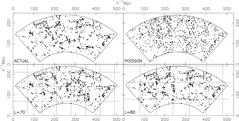
Figure 2: The data shown at top left, are the same as in Figure 1. The next panel (top right) shows a Poisson distribution of points generated over the same region. The bottom panels show Shuffled realizations of the data with $L=70$ and $80\,h^{-1}$Mpc. The square patches show the boundaries of the Shuffled regions While it is evident that the Poisson data are much less filamentarity than the LCRS galaxies, it is not possible to visually distinguish the level of filamentarity in the actual data from the Shuffled realizations. A quantitative analysis, shows that the $L=70\,h^{-1}$Mpc Shuffled data exhibit less filamentarity than the actual data, while the $L=80\,h^{-1}$Mpc Shuffled data are statistically identical to the original data in filamentarity (fig. 3). Note that all visual features across the boundaries in the bottom two panels (Shuffled data) are chance filaments.

Now we describe how the Shuffle algorithm works (Figure 2). A grid with squares of side $L$ is superposed on the original data slice. Square blocks of data which lie entirely within the slice are then randomly interchanged, with rotation, repeatedly, to form a new Shuffled slice. This process eliminates features in the original data on scales longer than $L$, keeping clustering at scales below $L$ nearly identical to the original data. All the structures spanning length-scales greater than $L$ that exist in the Shuffled slices are the result of chance alignments. For each value of $L$ we use different realizations of the Shuffled slices to estimate the degree of filamentarity that arises from chance alignments on scales larger than $L$. The Shuffled slices were analyzed in exactly the same way as the actual LCRS slices. At a fixed value of $L$, the average filamentarity in the original sample will be larger than in the Shuffled data only if the actual data have more filaments spanning length-scales larger than $L$, than that expected from chance alignments. We vary the value of $L$ from $10\,h^{-1}$Mpc to $100\,h^{-1}$Mpc and determine the largest value of $L$ ($L_{\rm MAX}$) such that for all $L<L_{\rm MAX}$ the values of the average filamentarity, ${\cal F}_{2}$, in the actual data are higher than the Shuffled data, indicating the presence of physical filaments of lengths greater than $L$. We use three realizations for $L=10,20,30,90$ and $100\,h^{-1}$Mpc shuffling of slices, and six realizations for the intermediate length-scales. For length-scales beyond $L_{\rm MAX}$ the average filamentarity in the Shuffled slices should continue to be the same as in the actual LCRS slice, establishing $L_{\rm MAX}$ to be the largest length-scale across which we have statistically significant filamentarity. Filaments which extend across length scales larger than $L_{\rm MAX}$ are not statistically significant and are a consequence of chance alignments. In Figure 3, we plot average filamentarity, ${\cal F}_{2}$, as a function of the filling factor, $FF$, for both the original sample as well as for samples generated by shuffling the patches for various values of $L$. To convey the essential aspects of the analysis, we only show the results for the slices shuffled at our lowest $L$ value, $L=10\,h^{-1}$Mpc and at or near the length-scale of interest, $L_{\rm MAX}$.

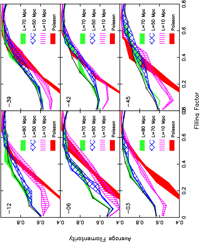
Figure 3: Plots of average filamentarity, ${\cal F}_{2}$, vs. Filling Factor, $FF$, for each of the LCRS slices (dark black line), three Shuffled realizations of each slice at various $L$ (hatched regions and light solid region)and three Poisson point distributions (dark solid region): We show Shuffle results for $L=10\,h^{-1}$Mpc, the smallest patches that were Shuffled, and the two L values where a transition occurs from the Shuffled galaxy distribution being less filamentary than the original data to it being indistinguishable from the original data. For each slice, this establishes $L_{\rm MAX}$, the length beyond which filaments are just chance artifacts, somewhere between these two values of $L$.

We use the $\chi^{2}$ test to establish $L_{\rm MAX}$ for the six individual slices. The reduced $\chi^{2}$ for the curves in Figure 3 are defined by

$$\chi^{2}(L)={1\over N_{B}-1}\sum_{i=1}^{N_{B}}\left[{{\cal F}_{2}^{(i),{\rm LCRS}}-{\cal F}_{2}^{(i),{\rm Shuffled}}(L)\over\sigma_{{\cal F}_{2}}^{(i)}(L)}\right]^{2},$$ (5)

where $N_{B}$ is the number of data points available for comparison between the original slice and a shuffled slice for a value of $L$. The quantity $\sigma_{{\cal F}_{2}}^{(i)}(L)$ is the standard deviation in ${\cal F}_{2}$ measured at a given filling factor, $FF_{i}$, using all the available shuffled realizations at a given length scale $L$. We have noted that for filling factor, $FF>0.7$, all the ${\cal F}_{2}$ curves follow the same trend, regardless of the slice (original or shuffled). This can be interpreted as the regime of $FF$ in which the coarse-graining defines structures of such large extent that they are unphysical and Shuffling does not discriminate between original or Shuffled data. Including the tiny differences in the curves in this regime ($FF>0.7$), will give weight to an unphysical signal and determine an erroneous $\chi^{2}$. Hence, we only include the region of the curves for $FF<0.7$ to determine the reduced $\chi^{2}$, using this as the discriminating measure between the curve for the real data and the Shuffled realizations at different $L$. The reduced $\chi^{2}$ quantifies how different a Shuffled slice is from the original, at various $L$. The minimum value of the reduced $\chi^{2}$ should correspond to the length-scale $L=L_{\rm MAX}$ at which, if slices are Shuffled, the filamentarity of the Shuffled slices and the original slice differ the least. This gives us the length scale $L_{\rm MAX}$ beyond which filaments are only chance objects and not physical.

Figure 4: The minimum value of the reduced $\chi^{2}$($L$) is plotted for all the six slices. It varies from 1.4 to 2.6 and is in within the acceptable bounds. We conclude from here that the scale of longest real filaments is $\sim 60\,h^{-1}$Mpc for all the three southern slices. For the northern slices this scale is $\sim 70-80\,h^{-1}$Mpc. This scale can also be interpreted as the scale beyond which the LSS in the Universe is homogeneous.

In Figure 4, we show the reduced $\chi^{2}$ vs. $L$ plotted for the six slices. We also list the minimum values of reduced $\chi^{2}$ for each slice and the corresponding $L$. We see that the values of reduced $\chi^{2}$ are well within acceptable bounds to say that the Shuffled slices at these values of $L$ are indistinguishable from the original slice. The length-scale that correspond to these minima is $\sim 60\,h^{-1}$Mpc for all the southern slices, whereas it is $\sim 70\,h^{-1}$Mpc for $-6^{o}$ slice and $80\,h^{-1}$Mpc for $-3^{o}$ and $-12^{o}$ slices. We thus establish that for the Southern slices the longest real filaments are no longer than $60\,h^{-1}$Mpc and for the Northern slices no longer than $80\,h^{-1}$Mpc. Beyond $80\,h^{-1}$Mpc structure is not statistically significant.

3 Discussion and conclusions

A look at the filamentary features at different levels of coarse-graining (Figure 1) reveals that the size of the largest filamentary feature increases monotonically with successive iterations of coarse-graining until it spans the entire survey (Bharadwaj et al. 2000). As coarse-graining proceeds, individual filaments form and then interconnect to form the supercluster-void network, in keeping with the earlier analysis (Einasto et al. 1984; Shandarin & Yess 2000; Einasto et al. 2003a) discussed in the introduction. Although, the length of the interconnected network of filaments increases monotonically, the ratio of the length to the number of holes (Genus) stabilizes and then decreases (Bharadwaj et al. 2000). For the $-3^{o}$ slice, this ratio stabilizes around $140\,h^{-1}$Mpc at $FF\sim$ 0.4. This ratio may be interpreted as the perimeter of the typical void in the network. This leads to a picture where there are voids of diameter $60\,h^{-1}$Mpc encircled by filaments of thickness $10\,h^{-1}$Mpc (Peebles 1993, Sheth et al. 2003, Sheth 2003) interconnected to form a large web. A void of this size, along with the filament at its perimeter, would span a length-scale $\sim 80\,h^{-1}$Mpc. The results of this paper show that such voids encircled by filaments are statistically significant features. Although our analysis also finds a web of interconnected filaments which spans length-scales larger than $80\,h^{-1}$Mpc and runs across the entire survey, this is not statistically significant. The web arises from chance interconnections between the filaments encircling different voids.

Studies of the distribution of Abell superclusters (Einasto et al. 1997b) show that the mean distance between neighboring superclusters is about $50\,h^{-1}$Mpc for poor superclusters and about $100\,h^{-1}$Mpc for rich superclusters. The distribution of the SDSS superclusters (Einasto et al. 2003a) and the LCRS superclusters (Einasto et al. 2003b) shows a similar behavior. Visualizing the superclusters as being randomly distributed, we would expect filaments joining the superclusters to develop as the density field is progressively smoothened. Such filaments will arise from the chance alignments of shorter, genuine, statistically significant filaments. The filaments joining superclusters will span length-scales comparable to the mean inter-supercluster separation and the statistical properties of filaments would be stable to shuffling i.e., it would not change if the superclusters were rearranged randomly. Our results may be interpreted as being indicative of the superclusters being randomly distributed on scales larger than $80\,h^{-1}$Mpc with the mean inter supercluster separation also being of this order .

The presence of statistically significant features on scales as large as $70$ to $80\,h^{-1}$Mpc may seem surprising given the fact that the correlation analysis fails to detect any clustering on scales beyond $30$ to $40\,h^{-1}$Mpc. This is due to the inability of the two point (and higher order) correlation functions in detecting coherence at large-scales. Pattern specific methods (like Shapefinders) are necessary to detect and quantify coherent large scale features in the galaxy distribution. It is interesting to note that the two dimensional power spectrum for the LCRS (Landy et al. 1996) exhibits strong excess power at wavelengths $\sim 100\,h^{-1}$Mpc, a feature which may possibly be related to the filamentary patterns studied here. The analysis of the three dimensional distribution of Abell clusters (Einasto et al. 1997a, 1997b) reveals a bump at $k=0.05\,h\,{\rm Mpc}^{-1}$ in the power spectrum. Also, the recent analysis of the SDSS shows a bump at $k=0.05\,h\,{\rm Mpc}^{-1}$ in the power spectrum (Tegmark et al. 2003). While it is interesting to conjecture that these features may be related to the presence of filaments, we should also note that the filaments are non-Gaussian features and cannot be characterized by the power spectrum alone.

A point which should be noted is that the filaments quite often run in a zig-zag fashion (Figure 1), and the length of a filament which spans a length-scale of $80\,h^{-1}$Mpc may be significantly larger than $80\,h^{-1}$Mpc. Also, the present analysis is two dimensional whereas the filaments actually extend in all three dimensions. The length of the filaments may be somewhat larger in three dimensions, and a little bit of caution may be advocated in generalizing our results .

In the gravitational instability picture, small disturbances in an initially uniform matter distribution grow to produce the large-scale structures presently observed in the universe. It is possible to interpret the filaments in terms of the coherence of the deformation (or strain) tensor (Bond, Kofman & Pogosyan 1996) of the smoothened map from the initial to the present positions of the particles which constitutes the matter. Our analysis shows that the deformation tensor has correlation to length-scales up to $80\,h^{-1}$Mpc and is uncorrelated on scales larger than this. The ability to produce statistically significant filamentarity on scales up to $80\,h^{-1}$Mpc will be a crucial quantitative test of the different models for the formation of Large Scale Structure in the universe.

We next address the question of the length-scale beyond which the distribution of galaxies in the LCRS may be considered to be homogeneous. The analysis of Kurokawa, Morikawa & Mouri (2001) shows this to occur at a length-scale of $\sim 30\,h^{-1}\,{\rm Mpc}$, whereas Best (2000) fails to find a transition to homogeneity even on the largest scale analyzed. The analysis of Amendola & Palladino (1999) shows a fractal behavior on scales less than $\sim$ $30h^{-1}\,{\rm Mpc}$ but is inconclusive about the transition to homogeneity. The results presented in this paper set a lower limit to this length-scale at around $80\,h^{-1}$Mpc, in keeping with estimates based on the multi-fractal analysis of LCRS (Bharadwaj, Gupta & Seshadri 1999) who find that the LCRS exhibits homogeneity on the scales $80$ to $200\,h^{-1}\,{\rm Mpc}$. In a separate approach based on the analysis of the two point correlation applied to actual data and simulations Einasto and Gramann (1993) find that the transition to homogeneity occurs at about $130\,h^{-1}{\rm Mpc}$. For the LCRS, the scale of the largest coherent structure is at least twice the length-scale at which the two-point correlation function becomes zero. Beyond this scale the filaments interconnect statistically to form a percolating network. This filament-void network of galaxies is not distinguishable, in a statistical sense, beyond scales of $80\,h^{-1}$Mpc. If the LCRS slices can be considered a fair sample of the universe then this suggests the scale of homogeneity for the universe.

4 Acknowledgment

The authors wish to thank the LCRS team for making the survey data public. SB would like to acknowledge financial support from the Govt. of India, Department of Science and Technology (SP/S2/K-05/2001). SPB would like to thank the Kentucky Space Grant Consortium (KSGC)for funding. JVS is supported by the senior research fellowship of the Council of Scientific and Industrial Research (CSIR), India. We also wish to thank the referee Jaan Einasto for providing very valuable and useful comments on our manuscript.

References

- (1) Abazajian, K., Adelman-McCarthy, J.K., Agueros, M.A., Allam, S.S. & the SDSS Collaboration, astro-ph/0305492
- (2) Amendola, L. & Palladino, E., 1999, ApJL, 514, 1
- (3) Barrow, J. D., Bhavsar, S. P., 1987, QJRAS, 28, 109
- (4) Best, J. S. 2000, ApJ, 541, 519
- (5) Bharadwaj, S., Sahni, V., Sathyaprakash, B. S., Shandarin, S. F. & Yess, C., 2000, ApJ, 528, 21
- (6) Bharadwaj, S., Gupta, A. K., Seshadri, T. R., 1999, A&A, 351, 405
- (7) Bhavsar, S. P., Ling, E. N., 1988, ApJL, 331, 63
- (8) Bond, J. R., Kofman, L., Pogosyan, D., 1996, Nature, 380, 603
- (9) Colless, M. et al. (for 2dFGRS team), 2001, MNRAS, 328, 1039
- (10) Colless et al. (for 2dFGRS team), astro-ph/0306581
- (11) Colley, W. N. 1997, ApJ, 489, 471
- (12) Doroshkevich, A. G., Tucker, D. L., Fong, R., Turchaninov, V., & Lin, H. 2001, MNRAS, 322, 369
- (13) Doroshkevich, A. G., Tucker, D. L., Oemler, A. J., Kirshner, R. P., Lin, H., Shectman, S. A., Landy, S. D., & Fong, R. 1996, MNRAS, 283, 1281
- (14) Einasto, J., H”utsi, G., Einasto, M., Saar, E., Tucker, D. L., M”uller, V., Hein”am”aki, P., Allam, S.S., 2003a, A&A, 405, 425
- (15) Einasto, J. et al. 2003b, A&A, 410, 425
- (16) Einasto, J. et al. 1997a, Nature, 385, 139
- (17) Einasto, M., Tago, E., Jaaniste, J., Einasto, J., & Andernach, H. 1997b, A&AS, 123, 119
- (18) Einasto, J. & Gramann, M. 1993, ApJ, 407, 443
- (19) Einasto, J., Klypin, A. A., Saar, E., & Shandarin, S. F. 1984, MNRAS, 206, 529
- (20) Geller, M. J., Huchra, J. P., 1989, Science, 246, 897
- (21) Kurokawa, T., Morikawa, M., & Mouri, H. 2001, A&A, 370, 358
- (22) Landy, S. D., Shectman, S. A., Lin, H., Kirshner, R. P., Oemler, A. , & Tucker, D. L., 1996, ApJL, 456, 1
- (23) Müller, V., Arbabi-Bidgoli, S., Einasto, J., & Tucker, D. 2000, MNRAS, 318, 280
- (24) Peebles, P. J. E., Principles of Physical Cosmology, Princeton University Press, 1993
- (25) Sahni, V., Sathyaprakash, B. S., & Shandarin, S.F., 1998, ApJL, 495, 5
- (26) Sathyaprakash, B.S., Sahni, V., Shandarin, S.F., & Fisher, K.B., 1998, ApJL, 507, 109
- (27) Shandarin, S. F. & Zel’dovich, I. B. 1983, Comments on Astrophysics, 10, 33
- (28) Shandarin, S. F. & Yess, C. 1998, ApJ, 505, 12
- (29) Shane, C. D., Wirtanen, C. A., 1954, AJ, 59, 285
- (30) Shectman, S. A., et al., 1996, ApJ, 470, 172
- (31) Sheth, J.V., Sahni, V., Shandarin, S.F., Sathyaprakash, B.S., 2003, MNRAS, 343, 22
- (32) Sheth, J.V., astro-ph/0310755, Submitted to MNRAS
- (33) Stoughton, C. et al. (for the SDSS collaboration), 2002, AJ, 123, 485
- (34) Tucker, D. L., et al., 1997, MNRAS, 285, 5
- (35) Zel’dovich, Ya. B., 1970, A&A, 5, 84
- (36) Tegmark, M., et al., 2003, ApJ, Submitted (astro-ph/0310725)
- (37) Trac, H., Mitsouras, D., Hickson, P., & Brandenberger, R. 2002, MNRAS, 330, 531
- (38) Zel’dovich, I. B., Einasto, J., & Shandarin, S. F. 1982, Nature, 300, 407